Proposing a New Evaluation Formula for Deep Hole Drilling Technique
Considering Three-dimensional Stress Fields
Houichi Kitano1, Shigetaka Okano2, and Masahito Mochizuki3
1 Graduate student, Dept. of Materials and Manufacturing science, Osaka University, Osaka, Japan
2 Assistantprofessor, Dept. of Materials and Manufacturing science, Osaka University, Osaka, Japan 3 Professor, Dept. of Materials and Manufacturing science, Osaka University, Osaka, Japan
ABSTRACT
The deep hole drilling (DHD) technique has received much attention in recent years as a method for measuring through-thickness residual stresses. However, some accuracy problems occur with the DHD technique. One reason is that the traditional evaluation formula assumes that the stress condition around the reference hole is two-dimensional plane stress. In this study, a new evaluation formula and procedure are proposed using three-dimensional stress functions to evaluate the residual stress more accurately. Then, a known stress field is evaluated by the traditional formula and the new formula using the finite element method to compare the accuracy of the both results. These results indicate that the proposed formula can evaluate the residual stress better than the traditional formula can.
INTRODUCTION
Residual stresses are found in weld joints because of the localized heat input, the difference between the expansion coefficients of joint members, and the restraints around the welded zones. In particular, high residual tensile stresses occur near welded zones. These stresses can affect the fracture and fatigue behaviors in welded structures Ohata et al (1986). Naturally, for assessing theses behaviors in detail, the inner residual stress fields are as important as surface residual stress fields. The neutron diffraction technique is a well-known evaluation method for the inner residual stress fields Park et al (2004). However, it is not always possible to easily conduct evaluations with this technique because it requires extensive experimental equipment and a stress-free sample. In addition, this technique cannot be applied to the residual stress evaluation of plates more than several tens of millimeters in thickness. Therefore, a new technique for evaluating inner residual stress fields is needed when the neutron diffraction technique cannot be applied.
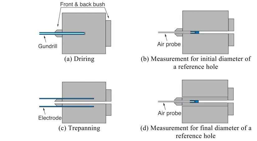
Consequently, the deep hole drilling (DHD) technique has received much attention in recent years as a method for measuring through-thickness residual stresses Leggatt et al (1996), Bouchard et al (2005) and Brown at al (2006). The DHD technique measures the diametric change of a reference hole drilled thorough the component before and after the residual stress release as in Figure 1. The DHD technique has some advantages over the neutron diffraction technique, such as simpler test devices and procedures, applicability to thick plates, and in-field testing capability. However, some accuracy problems occur with the DHD technique. One reason is that the traditional evaluation formula assumes that the stress condition around the reference hole is two-dimensional plane stress. Under this assumption, the stress conditions around the reference hole cannot be considered precisely. In addition, the effect of the residual stress distribution in thickness direction is ignored.
(a) Driring (b) Measurement for initial diameter of a reference hole
(c) Trepanning (d) Measurement for final diameter of a reference hole
Figure 1. Residual measurement procedure by deep hole drilling technique.
DIAMETRIC CHANGES OF THE REFERENCE HOLE UNDER THE THREE- DIMENSIONAL STRESS CONDITIONS
In this chapter, a new evaluation formula and procedure using three-dimensional stress functions are proposed. The effect of the stresses in thickness direction on the diametric changes, which are ignored in traditional evaluation formula, can be considered by using three-dimensional stress functions. The relationships !"#$""% displacement !,!,! and the three-dimensional functions, which are used in this study, are as follows:
i !=!!!
!" !=
1 !
!!!
!" ! =
!!!
!"
ii !=2 !
!!!
!" !=−2
!!!
!" ! =0
iii ! =!!!!
!" !=
!
!
!!!
!" !=!
!!!
!" − 3−4! !! iv ! =!!!!
!" !=0 !=−!
!!!
!" −4 1−! !!
v !=!cos!!!!
!" − 3−4! cos! !! !=cos!
!!!
!" + 3−4! sin! !!
!=!cos!!!!
!"
!!!
!=!!!!=!!!!=!!!!=!!!!=0
where, !,!,! are radial, circumferential and perpendicular displacements.
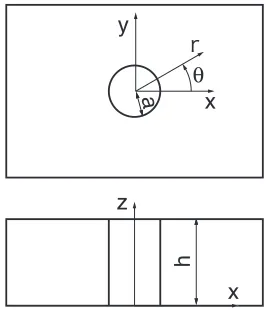
First developed are the relationships between the uni-axial stress fields σ(z) in the x direction, which have an arbitrary distribution in the z direction, and the diametric changes. The z direction is the thickness direction (0<z<h, h: thickness of object) and the x direction is the direction normal to the thickness direction as shown in Figure 2. Here, σ(z) can be expressed as a Fourier series
! ! =!!
2 + !!!!cos!!!! !!!!,!,!⋯
+ !!!!sin!!!!
!!!!,!,!⋯
(−!≤!!≤!,−
!
2≤!!≤ !
2) (1)
where !!=2!"/ℎ−! and !!=!!/2. In the following discussion, only the relationships between the
!!th stress of the second term on the right-hand side and the diametric changes are developed. This is because the effect of the third term on the right-hand side can be developed by most of the same procedure, and the effect of the first term on the right-hand side was already developed by Nakahara and Koizumi (1959).
Front & back bush
Gundrill Air probe
Figure 2. Definition of the cylindrical coordinate system.
Now, when there is no hole and the uni-axial load is !!=!!!!cos!!!!, the stress fields are as follows:
!!=
1
2!!!!cos!!!!(1+cos2!)
!! =
1
2!!!!cos!!!!(1−cos2!)
!!! =−
1
2!!!!cos!!!!sin2!,!!=!!! =!!"=0 The non-axisymmetric stress components are as follows:
!!=
1
2!!!!cos!!!!cos2!
!! =−
1
2!!!!cos!!!!cos2!
!!! =−12!!!!cos!!!!sin2!,!! =!!!=!!" =0
where, !! is the modified Bessel function of the second kind of order !. Now, let us define 2!"/ℎ and 2!"/ℎ as ! and !!, respectively. In addition when !!!!
!(!!!)[!′,!′,!′] is defined as
2!!!!
!!![!,! !], !, ! and ! can be determined as
! !
!
= !! !!!
!!
!!!
!!
!!! !!
!!!
!!
!!!
!! !!!
ℎ! !!!
ℎ!
!!!
ℎ!
!!! !!
− 1 4! 0 1 4!
(2)
where,
!!=!!!
!! !!!!
!! !!!! + !!!! !+6,!!=− !!!! ! !!!
!! !!!!
!! !!!! + 1+2! ,
ℎ!=−4 !!!!!! !!!!
!! !!!! +3 ,!! =!!!!
!! !!!!
!! !!!! +2,
!!=2 1−! !!!!
!! !!!!
!! !!!! − !!!!
!+2 1−2! ,
ℎ! =−2,!!=2 !!!!!! !!!!
!! !!!! +3 ,
!! =− !!!! !,ℎ
!=− 2!!!
!! !!!!
!! !!!! + !!!! !+12 . x
y
z
θ
x
h
When !, ! and ! are determined by Equation 2, the stress components in the thickness direction can also be determined.
!! !!!±!
2!!!!!
!!!cos2! = −
!! !! !!!
!! !!!! −!+ !!!
!! !!!
!! !!! −2 1−! !
!!!=!!" =0
On the surface (!! =±!), !! has to be zero. Therefore, the following additional stress functions are
used.
[Stress function I]
2!!! =!!!!! cos2!
!! +!!!log!
2!!!=!!!! cos2!
!! ,2!!!=!!!!
cos2!
!! ,2!!!=!!!
cos2!
!
[Stress function II]
2!!!= !!!!! !" cos!"cos2!
!
2!!!= !!!!!! !" sin!"cos2!
!
2!!! = !!!!! !" cos!"sin2!
!
[Stress function III]
2!!!= !!! !! !" cosh!"cos2! !
2!!!= !!!! !! !" sinh!"cos2! !
where, !! !" =!! !" −{!!(!")/!! !" }!!(!"), !!: the Bessel function of the first kind of order !, !!: the Bessel function of the second kind of order !. Here, m is the value that satisfies
!! !! =!! !" =0 (!≫!), and !!,!!,!!⋯ are defined as the numbers of ! in ascending
order. The stresses, which are obtained by these functions, have to satisfy the following boundary conditions:
At !=∞, all stress components are zero. At !=!, !! =!!"=!!! =0.
At !!=±!, !!!=!!"=0,
!! !!!±!
2!!!!!
!!!cos2!= −
!! !! !!!
!! !!!! !− !!!
!! !!!
!! !!! −2 1−! ! .
Here, when !!! is determined as !!! 1−2!−!"cot!" , – − !!!!![!!!,!!!,!!!] is defined as 2!!!!
!!![!!,!!,!!] and 4!! !"#$!"
!" !!! is defined as 2!!!!!!!!!, the relationships of the
coefficients obtained by the boundary condition on the hole surface (!=!) are as follows:
!!! !!!
!!! !!! !!! !!!
!!! !!!
!!! !! !!
!! =
!!!"!!
!
!!!"!!
!
!!!"!! !
! =!=0,1!,2,3,⋯
!,!!,⋯ (3)
where,
!! =!!(!!!), !!!=!!!!!!
!+ !!!
!+6,
!!!=!!!!!
!!+2,!!!=2 !!!
!! !!+3 ,
!!!=− !!! ! !!!
!!
!!!=2 1−! !!!!!
!!− !!! !+2 1−2! , !!!=− !!! !, !!! =−4 !!!!!!!+3 ,!!!=−2,
!!!=−2 !!!
!! !!+
!!! ! 2 +6 ,
!!!" =!!!"+ !" !
2 !!!",!!!!=1, !!!"=−2 !!!!
!!+!! !,!!!!=0,
!!!"=−3 1−! !
!!−! !!!",!!!"=1.
In addition, the relationships of the coefficients obtained by the boundary condition on the surface (!=±!) are as follows:
!! !!!±!
2!!!!!
!!!cos2!=− 1 !!
1+!
12 +
1
!![!!!! !" !
−!! !"!! !" −2 1−! ]
−1 4
!! !! !
!"
sinh!" cosh!"+ !"
sinh!" !!(!")
= − !! !! !!!
!! !!!! !− !!!
!! !!!
!! !!! −2 1−! !
(4)
and where, !!=!!(!!!). Now, !!(!")and !"!!(!") are expanded in the Fourier-Bessel series
!! !" =
!!!
!! + !!"!! !" !
!"!! !" =
!!!
!! + !!"!!(!") !
where,
!!! =
!!!! !!!−!
!!
2
! !!!! !!! +!!!! !!! !!"=
1 !!!!
! !!! −!!!!! !!!
2
!!+!! !!!!! !!! !! !!! −!!!!! !!! !! !!!
!!!=
2!!!! !!
!!!−! !!
!! !!! −!! !!! ,
!!" =
1 !!!!
!! !!! −!!!!!! !!!
2 !!+!!
[{ !!! !!! !!! !! !!! − !!! !!! !!! !! !!! }
− 4− 2!!
!!+!! !!!!! !!! !! !!! −!!!!! !!!)!! !!! . and where, !!≫!!. Here, the coefficients of 1/!! and !
!(!") are to be zero in Equation 3. Therefore, using Equation 3 and Equation 4:
!!!!!=!!!
!
+!!!!!, !!"!! =!!! +!!!!
!
where,
!!!= − !! !!
!!!!−!!!!!! ,!!! = − !! !!!! !!−!!!! !! ,
!!=1+!
12 !!!,!! =
1 4
!"
sinh!" cosh!"+ !"
sinh!" 1
!!
!!! = !!"!!!!−!!"! !!!! , !
!!"= !!"!!"! −!!"! !!"! , !
!!!!= !!!
!! ,!!"
!!!! = !!! !! −
2 1−! !!! !! ,!!"
! = !!" !! −
2 1−! !!" !! . Here, !!",!!"! are the values that satisfy !
!= !!!"!!,!!= !!!"! !!. Therefore, these are
obtained from Equation 3. Secondly, axisymmetric stress components are as follows:
!!=
1
2!!!!cos!!!!,!!= 1
2!!!!cos!!!!
!! =!!!=!!"=!!!=0
Here, the stress functions for the boundary condition on the hole surface (!=!) are as follows:
2!!!= !!
!!!! !" cos!",2!!!=
!!
! !! !" sin!"
In addition when !![!!,!!] is defined as 2!!!!![!,!], ! and ! can be determined as
! ! = !! !! !! !! !! − 1 4! 0 (5) where, !!=!!! !+ 1
!!!!,!!=−!!!!+ 1−2! !!
!!, !!=−1,!! =2 1−! −!!!!!!
!!.
When ! and ! are determined by Equation 5, the stress components in the thickness direction can also be determined.
!! !!!±!
2!!!!!!!cos2!
=− − !!!! !!!
!! !
!! !!!
!! !!! −! !!!−2(2−!)
!! !!! !! !!!
!!!=!!" =0
On the surface (!! =±!), !! has to be zero. Therefore, the following additional stress functions are used.
[Stress function I]
2!!! =
!!!
!!!! !" cos!"
!
,2!!!=
!!!
! !! !" sin!" !
[Stress function II]
2!!!= !!!
!!!! !" cosh!", !
2!!! = !!! !
! !" sinh!" !
The stresses, which are obtained by these functions, have to satisfy the following boundary conditions:
At !=∞, all stress components are zero.
At !=!, !!=!!"=!!! =0.
At !!=±!, !!!=!!"=0,
!! !!!±!
2!!!!!!!cos2!
= − !!!! !!!
!! !
!! !!!
!! !!! −! !!!−2(2−!)
!! !!! !! !!!
Here, when !!! is determined as !!! 1−2!−!"cot!" , !!![!!!,!!!] is defined as 2!!!!![!!,!!]
and 2!!!"#$!"!" !!! is defined as 2!!!!!!!, the relationships of the coefficients obtained by the
boundary condition on the hole surface (!=!) are as follows:
!! !!
!! !!
!!
!! =
!!!!" !
!!
0
!=!=0,1!,2,3,⋯
!,!!,⋯ (6)
where,
!! =
!! !!+
1
!!!,!!=−!!!+ 1−2!
!! !!,
!! =−1,!!=2 1−! −!!!
!! !!,!!!"
! =− 2!!
In addition, the relationships of the coefficients obtained by the boundary condition on the surface (!!=±!) are as follows:
!! !!!±!=−
1
!! −!!!!+!! !"!! !" −2 2−! !!(!")
!
− !! !"
!!
!"
2!!sinh!" cosh!"+
!"
sinh!" !!
!
=− − ! 1
!![−!!! !!! +! !!!!! !!! −2 2−! !!(!!!) ]
(7)
Now, !!(!") and !"!!(!") are expanded in the Fourier-Bessel series
!! !" = !!"!! !! !" !
,!"!! !" = !!"!! !!(!") !
where,
!!"!! = 2! !!+!! !
!! !!! !!!−!!! !!! !!!
!! !!! !! !!! !! −!! !!! !! !!! !!
!!"!! =
2!!
!!+!! !
!! !!! !!!−!!! !!! !!!
{!! !!! !! !!! !!!−!! !!! !! !!! !!!
+2 !! !!! !! !!! !!−!! !!! !! !!! !!
!!+!! }
Now, the coefficients of !!(!") are to be zero in Equation 7. Therefore, using Equation 6 and Equation 7,
!!"! !
!=!!! +!!!!
!
where,
!!! = − !! !!!!!!"+!!!"!!! ,!! =
!"
2!!sinh!" cosh!"+
!"
sinh!" 1
!!,
!!"! = !!"!!!!!!!"+!!"!!!!!"!!! , !
!!"!!! =−!!" !!
!! ,!!"!!! = !!"!!
!! −2(1−!) !!"!!
!!
Here, !!"!!,!!"!!! are the values that satisfy !!= !!!"!!!!,!! = !!!"!!!!!. Therefore, these are
obtained from Equation 6.
The coefficients of each stress functions are determined uniquely according to the above discussion. Now, the displacement of the hole edge is determined as follows:
− !
!!!!!!! !,! =+ [
− !!!
!! [− !!!
!! !!!
!! !!! +2 !! !
+ !!! !!!+4!!]cos!!!cos2!
!! 3
− !
!! cos!!!
!
− !!! !! −
!!!
12
1+2! 1−2!!!
!
cos2!+{ !!!
!! + − !!! !! !!+!! ! ! !
2!−1+!
!−!!
!!+!! cos!!!}cos2!−
1
!![ !!!!
!! !!!!
!! !!!! +2 !− !!!!
!!
−4!]cos!!!!cos2!+
cos!!!!cos2!
4! + − !!!
1 !!!!!+
!! !!!
!! !!! !! cos! !!
!
− 1
!!!!−
!! !!!! !! !!!! !−
1−!
2! 1+! cos!!!!
In addition, when the diametric changes caused by the uni-axial stress fields !(!) are denoted by
!!"#$% !!,!!,!!",!,! =!!"#$%& !!,!,! +!!"#$%& !!,!,!− ! 2 + !!"#$%& !!",!,!−!
4 +!!"#$%& !!",!,!+ ! 4
(8)
When Equation 8 is applied to the residual stress evaluation using the DHD technique, the residual stress fields are the stress fields that satisfy Equation 8 using !!"#$% obtained by the DHD process.
METHOD FOR EVALUATING RESIDUAL STRESS CONSIDERING THREE-DIMENSIONAL STRESS FIELDS
The diametric changes can be calculated from the residual stress fields by using Equation 8. Therefore, the residual stress fields can be calculated from the diametric changes obtained by thr DHD procedure as follows:
1. Calculate !! !, !! !, !!" ! from the diametric changes ! by using Equation 9. 2. Calculate !!"#$% ! from !! !, !!
!, !!" ! by using Equation 8.
3. Calculate the differences between !" =!− !!"#$% ! .
4. Calculate !!!,!!!,!!!" by using Equation 10.
5. Calculate !!"#$% !!! from !! !!!, !! !!!, !!" !!!.
6. When !">!(!: convergence criteria), go back to 3. Afterwards, ! is replaced to !+1.
! !,! =−1
![!! 1+2cos2! +!! 1−cos2! +!!" 4sin2! ] (9)
!" !,! =−1
![!"! 1+2cos2! +!"! 1−cos2! +!"!" 4sin2! ] (10)
EVALUATION OF A RESIDUAL FIELD BY PROPOSED AND TRADITIONAL FORMULAE
The object used for the FEM is shown in Figure 3. The initial diameter of the reference hole is 2 mm, and the outside diameter of the trepanned cylinder is 4 mm. The size of the mesh in the radial direction around the reference hole is approximately 0.03 mm. The thickness is divided into 1000 meshes and the arc is divided into 144 meshes. In this analysis, the object is assumed to have an elastic body (Young’s modulus: 200 GPa, Poisson’s ratio: 0.3) and the residual stress is applied in the x direction. The distribution is represented by a quadratic function that has maximum values at the surfaces of the object and a minimum value at the middle of the object. The absolute values of the these values are 300 MPa. Under these conditions, the DHD procedure is simulated as shown in Figure 4.
(a) Size of whole model (b) Size around the reference hole
Figure 3. Object used for FE analysis.
: Fixed plane in all directions
x y z
50
30
30 Symmetrical
planes
(unit: mm)
1
3
2 Cylinder
(a) Definition of axes and a legend (b) After stress loading
(c) After drilling (d) After Trepanning
Figure 4. Simulated DHD procedure by FE analysis.
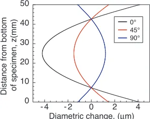
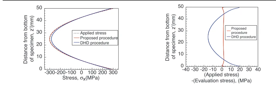
The diametric changes for the residual stress evaluation are obtained at the angles of 0°, 45° and 90° by using the result of the FEM as shown in Figure 5. In the evaluation by the traditional and the proposed formulae (Equation 8), !! and !!" are not fixed to zero. The evaluation results obtained by both formulae and the applied stress are shown in Figure 6. The errors of both evaluation results, which are calculated by (Applied stress)-(Evaluated stress), are shown in Figure 7. These results indicate that the proposed formula can evaluate the residual stress better than the traditional formula can.
Figure 5. Diametric changes obtained by FEM.
0° 45° 90°
Figure 6. Evaluation results obtained by both procedures.
Figure 7. Errors of results obtained by both procedures.
CONCLUSION
A new evaluation formula that considersthe effects of the three-dimensional stress condition was presented. The evaluation results obtained by the proposed formula agree with the applied stress better than those obtained by the traditional formula.Using the proposed formula, the DHD technique can evaluate residual stresses more accurately.
REFERENCES
Ohata, A., Maeda, Y., Mawari, T., Nishijima, S. and Nakamura, H. (1986) “Fatigue strength evaluation of welded joints containing high tensile residual stresses,” International Journal of Fatigue, 8, 147–150.
Park, M. J., Yang, H. N., Jang, D. Y., Kim, J. S. and. Jin, T. E(2004) “Residual stress measurement on welded specimen by neutron diffraction,” Journal of Materials Processing Technology, 155-156, 1171–1177.
Leggatt, R. H., Smith, D. J., Smith, S. D. and Faure, F. (1996) “Development and experimental validation of the deep hole method for residual stress measurement,” The Journal of Strain Analysis for Engineering Design, 31. 177-186
Bouchard, P., George, D., Santisteban, J., Bruno, G., Dutta, M., Edwards, L., Kingston, E. and Smith, D. (2005) “Measurement of the residual stresses in a stainless steel pipe girth weld containing long and short repair,” International Journal of Pressure Vessels and Piping, 82, 299-310. Brown, T., Dauda, T., Truman, C., Smith, D., Memhard, D. and Pfeiffer, W. (2006) “Predictions and
measurements of residual stress in repair welds in plates,” International Journal of Pressure Vessels and Piping, 83, 809-818.
Nakahara, I. and Koizumi, T. (1959) “The effect of plate thickness on the stress distributions around a circular hole in an infinite plate subjected to uniaxial tension,” Transactions of the Japan Society of Mechanical Engineers, 125-151, 181-189 (in Japanese).
Applied stress Proposed procedure DHD procedure
Stress, σx(MPa)
Distance from bottom of specimen, z’(mm)
Proposed procedure DHD procedure