SkyPackage: From Finding Items to Finding A Skyline of Packages on the Semantic Web.

(1)

ABSTRACT

SESSOMS, MATTHEW WADE. SkyPackage: From Finding Items to Finding A Skyline of Packages on the Semantic Web. (Under the direction of Dr. Kemafor Anyanwu.)

Enabling complex querying paradigms over the wealth of available Semantic Web data will significantly impact the relevance and adoption of Semantic Web technologies in a broad range of domains. While the current predominant paradigm is to retrieve a list of items, in many cases the actual intent is satisfied by reviewing the lists and assembling compatible items into lists or packages of resources such that each package collectively satisfies the need, such as assembling different collections of places to visit during a vacation. Users may place constraints on individual items, and the compatibility of items within a package is based on global constraints placed on packages, like total distance and time to travel between locations in a package and total cost. Finding such packages using the traditional item-querying model requires users to review lists of possible multiple queries and assemble and compare packages manually.

(2)

(3)

SkyPackage: From Finding Items to Finding A Skyline of Packages on the Semantic Web

by

Matthew Wade Sessoms

A thesis submitted to the Graduate Faculty of North Carolina State University

in partial fulfillment of the requirements for the Degree of

Master of Science

Computer Science

Raleigh, North Carolina 2012

APPROVED BY:

Dr. Christopher Healey Dr. Nagiza Samatova

(4)

DEDICATION

(5)

BIOGRAPHY

(6)

ACKNOWLEDGEMENTS

(7)

LIST OF TABLES

(10)

LIST OF FIGURES

Figure 2.1 Skyline of Hotels . . . 5

Figure 2.2 RDF Graph . . . 8

Figure 2.3 Data For E-Commerce Example . . . 10

Figure 2.4 Dataflow for the SkyPackage Problem in Terms of Traditional Query Operators . . . 11

Figure 3.1 Cartesian Product of Join Result . . . 17

Figure 3.2 Cartesian Product Result . . . 17

Figure 3.3 RSJ F H (skyline-over-join) for milk . . . 20

Figure 3.4 RSJ F H’s result for milk . . . 20

Figure 3.5 Cartesian product on all targets (e.g., milk, eggs, and bread) . . . 20

Figure 3.6 E-commerce Data . . . 22

Figure 3.7 Skyline Region . . . 26

Figure 3.8 Pruning Example . . . 27

Figure 3.9 Pruning and Early Termination Result . . . 29

Figure 3.10 Skyline Package Result . . . 29

Figure 4.1 Sesame Components . . . 32

Figure 4.2 MovieLens Ontology . . . 33

Figure 4.3 Framework with SPARQL Adapter . . . 34

Figure 4.4 Queries to construct target qualifying tables . . . 36

Figure 4.5 Query to construct target descriptive table . . . 36

Figure 5.1 Synthetic Data Triple Sizes . . . 39

Figure 5.2 Evaluation Results for Package Sizes 2 and 3 . . . 40

Figure 5.3 Evaluation Results for Package Sizes 4 and 5 . . . 41

Figure 5.4 Scalability for Package Sizes 2 to 5 . . . 43

Figure 5.5 Prunability of Synthetic Data . . . 44

Figure 5.6 Package Size Scalability for MovieLens . . . 45

Figure 5.7 Prunability of MovieLens Dataset . . . 46

Figure 5.8 Package Size Scalability for Book-Crossing . . . 47

Figure 5.9 Prunability of Book-Crossing Dataset . . . 48

Figure 5.10 Database build for Synthetic Data . . . 49

Figure 5.11 Database build for MovieLens Data . . . 49

(11)

Chapter 1 Introduction

The traditional search and querying paradigms on the Web are aimed towards a sin-gle item being the focus of a user’s item search. With the Semantic Web envisioning documents from different origins being linked together, the data becomes more useful enabling data from different sources to be connected and queried. The surge in interest and availability of structured data on the Semantic Web provides an opportunity to in-vestigate more advanced querying paradigms that are useful for different kinds of tasks, specifically finding a combination or package of items satisfying a user’s preference.

Skyline queries, a common type of preference queries, focuses on finding the best set of objects, with repect to the user’s preferences, from the given data. Current research focuses primarily on skyline sets whose elements have cardinality of one. The Semantic Web allows for more advanced searches involving not only single-item sets, but also multi-item sets (i.e., packages). The main challenge in terms of package skylines is dealing with the exponential increase in the search space due to the combinatorial explosion.

1.1 Thesis Motivation

(12)

meaning the goal of the query is to find candidate combinations or “packages.” Finding such packages using the traditional item querying model requires users to review lists of results for possibly multiple queries and then manually combining these into suitable packages which can be very tedious.

To illustrate another example, consider Samantha, who is in the 8th grade, is having difficulty grasping the concepts of mathematics. She wishes to pursue additional help by means of e-learning and is interested in videos that cover quadratic equations, linear functions, and scatterplots. Each video, i.e., a resource, has properties such as rating and video length. She is willing to spend up to 45 minutes each day using an e-learning system and prefers the average rating of all the videos to be high. Hence, Samantha is interested in a package of three e-learning resources whose total property value for length is less than 45 and whose average property value for rating is high.

These examples show that the target of the query is in fact a set of items (a set of stores, a set of learning sessions), where the query should return multiple combinations or “package”. Finding such packages using the traditional item querying model requires users to review lists of results for possible multiple queries and then manually combining these into suitable packages. The examples also demonstrate the need to support mul-tiple selection criteria for packages. Furthermore, selection criteria could involve hard constraints, such as a total price for the package is less than $500, or soft constraints, such as preferring a minimally priced item.

1.2 Key Contributions

To our knowledge, we are the first to study package skyline queries. In this thesis, we propose the concept of package skyline queries and an approach for evaluating such queries. Specifically, we contribute the following:

1. A formalization of the concept of package skyline queries over an RDF data model 2. An efficient storage model for making such queries easier to answer.

3. An efficient technique for evaluating package skyline queries on an RDF database 4. An approach for a loose integration of this technique in an open source RDF

(13)

1.3 Thesis Organization

The remaining thesis is organized as follows:

(14)

Chapter 2 Background and Related Work

This chapter introduces preference queries and a type of preference query known as sky-line queries. It also provides some definitions and concepts that will be used throughout this thesis. Finally, we provide related work.

2.1 Preference Queries

Preferences, such as “I like A more than B,” can be easily stated by users when asked for their wishes. For example, when purchasing a car, it is easy to state a preferred color and that a car with high gas mileage is more desirable than one with lower gas mileage. Preferences consists ofsoft constraintsandhard constraints. A hard constraint represents an absolute limitation on the choices at hand, while a soft constraint is neither required nor necessary, but desired. If a preference query contained only hard constraints, it is likely that the search results would not yield many, if any, exact matches, forcing a low number of results, and thus soft constraints are more suitable for users.

Preference-based querying [17][25][36] involves presenting users with a set of best

(15)

Figure 2.1: Skyline of Hotels

2.1.1 Skyline Queries

A classic example used to illustrate the concept of skyline queries is searching for cheap hotels close to the beach. Suppose John and his family are visiting the beach for a weekend vacation and are interested in finding a hotel that is close to the beach and has a low price. If hotel h1 is closer to the beach and has a cheaper price than hotel h2, it

is obvious that h1 is a better choice than h2. In this case, h1 is said to dominate h2 in

both price and distance. If h1 is cheaper than h2 but is located farther away from the

beach, h1 and h2 are called incomparable (neither is better assuming equal weight on

preferences).

A sample set of hotels is depicted in Figure 2.1 (borrowed from [10]), characterized by two dimensions, distance and price. A hotel belongs in the skyline if there are no other hotels that are better than it in both dimensions, i.e., both cheaper and closer to the beach. Similarly, a hotel appears in the skyline if, at a given distance from the beach, no hotel is cheaper, or conversely if, at a given price, no hotel is closer to the beach. The distinguishing property of the skyline is that for any preference function f

(16)

function that is maximized by this object. Intuitively, this means that (a) regardless of how a user weighs his/her preferences, his/her top preferred object will be one of the skyline objects, and (b) there is no skyline object which is nobody’s top preference. The skyline is formally defined next.

Definition 2.1.1 (Dominance) Let p= (p1, . . . , pd)andp0 = (p01, . . . , p

0

d)be two points in Rd_{. Point} _p _dominates _p0 _{(denoted as} _p _p0_{) if and only if} _p

i is better than or equal

to p0_i for 1≤ i ≤d and pj is strictly better than p0j for some 1 ≤ j ≤d. The total order

is reflexive, antisymmetric, transitive, and comparable (totality).

In other words, given a set of points, a point dominates another point if it is as good or better in all dimensions and better in at least one dimension.

Definition 2.1.2 (Skyline Set) The set of all non-dominated points.

The problem of finding all such points is called the skyline query problem

2.2 Semantic Web

The original Web was designed to provide information in a human-readable format, which meant machines could not process or reason about the data. Queries asked to the Web (e.g., who performed this piece of music?) could not be answered. Although web mining tools were researched and proved useful in some situations, no extraction algorithm is robust enough to handle every domain. An approach to circumvent this limitation is to make the data explicit on the Web in a way which allows machines to process the information. This approach was the first step towards the Semantic Web. Tim Berners-Lee defines this term as follows:

The Semantic Web is not a separate web but an extension of the cur-rent web, in which information is given well-defined meaning, better enabling computers and people to work in cooperation. [8]

(17)

2.2.1 RDF Data Model

Resource Description Framework (RDF) [29], a W3C recommendation, is a directed, la-beled graph data model for asserting statements about resources. The Web is built around the concept of Uniform Resource Identifiers (URI) [7]. A URI can identify any-thing, from a document to a person, a performance, an audio signal, etc. Statements, or facts, are expressed in this data model using triples, where each triple consists of a

subject,predicate, and anobject. It is common to refer to anRDF statementas asubject

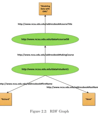
having a property name whose value is the property value, e.g., object, which may be a literal or another resource. A set of triples may be depicted as a graph of resources whose edges represent the binary relationships between them. As an example, Figure 2.2 shows an RDF graph containing four RDF statements. In this example, the graph asserts the statement that “Richard Mutt is taking the course ‘Modeling Data with OWL’.” Using common notation, ellipses denote resources and squares denote literals. If a shorthand notation is used to reduce the full URI reference, http://www.ncsu.edu.edu/data# and http://www.ncsu.edu.edu/addressbook# can be represented as “d:” and “ab:”, respec-tively. This statement can be represented in triple notation (subject, predicate, object), as shown in Table 2.1.

2.2.2 SPARQL

RDF can be serialized into many different formats, such as XML [3], N3 [30], Turtle [4], and N-Triples [19]. Although the N3, Turtle, and N-Triples formats are often more concise and presented in a more human-readable format, the XML form of RDF, i.e., RDF/XML, is the preferred syntax. Several techniques for querying XML documents exist, but with the Semantic Web in mind, the interest is not in querying at thesyntactic

level but querying at the semantic level [14]. In order to query the Semantic Web, a query language that recognizes the semantics of RDF is needed. Several such languages

Table 2.1: Triple notation for Figure 2.2 (d:student1, ab:firstName, “Richard”)

(d:student1, ab:lastName, “Mutt”)

(d:student1, ab:takingCourse, d:course59)

(18)

http://www.ncsu.edu.edu/data#student1 http://www.ncsu.edu.edu/data#course59

“Richard” “Mutt”

“Modeling Data with

OWL”

http://www.ncsu.edu.edu/addressbook#courseTitle

http://www.ncsu.edu.edu/addressbook#takingCourse

http://www.ncsu.edu.edu/addressbook#lastName http://www.ncsu.edu.edu/addressbook#firstName

(19)

exist [13][22][35][37][38], but we focus on SPARQL [21] (a recursive acronym for SPARQL Protocol and RDF Query Language) because it is the current W3C recommendation for querying RDF data.

Using the RDF graph in Figure 2.2 as an example, we wish to find which course(s) Richard Mutt is taking. One can answer this query by executing a simple SPARQL query, which has an SQL-like syntax, in the following manner, where variables are prepended with “?”.

SELECT ?course

WHERE { ?student ab:firstName "Richard".

?student ab:lastName "Mutt".

?student ab:takingCourse ?course.

}

2.3 Motivating Example

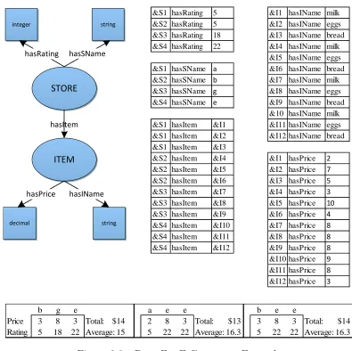
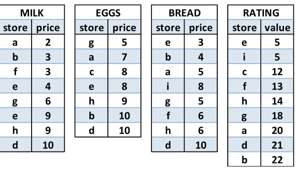
Now that some background material has been introduced, we can provide some more insight into our motivating example. Revisiting the shopping list example from Chapter 1, the shopper poses the following query in Query 2.3.1.

Query 2.3.1 I want to purchase milk, eggs, and bread (one of each) from one or more stores such that the total price is minimized and the average rating of the stores is

maximized.

(20)

ITEM STORE hasItem string integer decimal hasRating hasSName string hasPrice hasIName

&S1 hasRating 5 &I1 hasIName milk &S2 hasRating 5 &I2 hasIName eggs &S3 hasRating 18 &I3 hasIName bread &S4 hasRating 22 &I4 hasIName milk

&I5 hasIName eggs &S1 hasSName a &I6 hasIName bread &S2 hasSName b &I7 hasIName milk &S3 hasSName g &I8 hasIName eggs &S4 hasSName e &I9 hasIName bread

&10 hasIName milk &S1 hasItem &I1 &I11 hasIName eggs &S1 hasItem &I2 &I12 hasIName bread &S1 hasItem &I3

&S2 hasItem &I4 &I1 hasPrice 2 &S2 hasItem &I5 &I2 hasPrice 7 &S2 hasItem &I6 &I3 hasPrice 5 &S3 hasItem &I7 &I4 hasPrice 3 &S3 hasItem &I8 &I5 hasPrice 10 &S3 hasItem &I9 &I6 hasPrice 4 &S4 hasItem &I10 &I7 hasPrice 8 &S4 hasItem &I11 &I8 hasPrice 8 &S4 hasItem &I12 &I9 hasPrice 8 &I10 hasPrice 9 &I11 hasPrice 8 &I12 hasPrice 3

b g e a e e b e e

Price 3 8 3 Total: $14 2 8 3 Total: $13 3 8 3 Total: $14 Rating 5 18 22 Average: 15 5 22 22 Average: 16.3 5 22 22 Average: 16.3

Figure 2.3: Data For E-Commerce Example

Figure 2.3 shows the total price and average rating for packagesaee,beeandbge. We see that aee is a better package than bee because it has a smaller total price and the same average rating. On the other hand,bgeandaee are incomparable because althoughbge’s total price is worse than aee’s, its average rating is better.

(21)

SELECT ?s ?price ?rating ?store WHERE ?store :hasSName ?s

?store :sells ?item ?store :hasRating ?rating ?item :hasIName “milk” ?item :hasPrice ?price

?store :sells ?item ?store :hasRating ?rating ?item :hasIName “bread” ?item :hasPrice ?price

?store :sells ?item ?store :hasRating ?rating ?item :hasIName “eggs” ?item :hasPrice ?price

UNION UNION

s1 5 &I1 milk $2 s1 5 &I3 bread $5 s1 5 &I2 eggs $7 s1 5 &I1 milk $2 s1 5 &I3 bread $5 s2 5 &I5 eggs $10

…

s1 s1 s1 $14 5 s1 s1 s2 $17 5

… s1 5 &I1 milk $2

s2 5 &I4 milk $3 …

s1 5 &I3 bread $5 s2 5 &I6 bread $4

…

s1 5 &I2 eggs $7 s2 5 &I5 eggs $10

…

´

_´

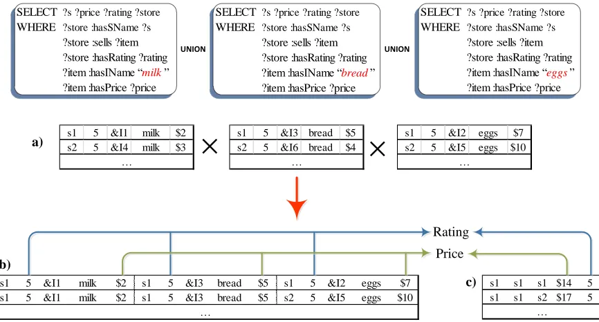
a) Rating Price c) b)

Figure 2.4: Dataflow for the SkyPackage Problem in Terms of Traditional Query Oper-ators

specified over the aggregates of target attributes (datatype properties), e.g., maximizing the average over store ratings, as well as the attributes of target qualifiers, e.g., minimiz-ing total price. Note that the resultminimiz-ing graph pattern structure (we ignore the details of preferences specification at this time) involves a union query where each branch computes a set of results for one of the target qualifiers, as shown in Figure 2.4.

We now provide a more formal presentation of SkyPackage graph pattern queries.

2.4 Problem Definition

LetDbe a dataset with property relationsP1,P2, .., Pm andGP be a graph pattern with

triple patterns T Pi, T Pj, .., T Pk (T Px means triple pattern with property Px). [[GP]]_D

denotes the answer relation for GP over D, i.e., [[GP]]_D = Pi no Pj on ... on Pk. Let var(T Px) andvar(GP) denote the variables in the triple and graph pattern respectively.

We designate the return variable r ∈ var(GP), e.g., (?store), representing the target of the query (stores) as the target variable. We call the triple patterns such as (?item,

(22)

We review the formalization for preferences given in [32]. Let Dom(a1), . . . Dom(ad)

be the domains for the columns a1, .., ad in a d-dimensional tuple t ∈ [[GP]]_D. Given a

set of attributes B ⊆ A0, a preference P F over the set of tuples [[GP]]_D is then defined asP F := (B;≺P F), where ≺P F is a strict partial order on the domain ofB. Given a set

of preferences P F1, ..., P Fm, their combined Pareto preference P F is defined as a set of

equally important preferences.

For a set of d-dimensional tuples R and preference P = (B;≺P) over R, a tuple ri ∈ R dominates tuple rj ∈ R based on the preference P (denoted as ri≺Prj), iff

(∀(ak∈B)(ri[ak]≺₋ rj[ak])∧ ∃(al∈B)(ri[al]≺rj[al]))

Definition 2.4.1 (Skyline Query) When adapting preferences to graph patterns we associate a preference with the property (assumed to be a datatype property) on whose

object the preference is defined. Let P Fi denote a preference on the column representing the object of property Pi). Then, for a graph pattern GP = T P1, .., T Pm and a set of

preferences P F = P Fi, P Fj, .., P Fk, a skyline query SKY LIN E[[[GP]]D, P F] returns the set of tuples from the answer of GP such that no other tuples dominate them with

respect to P F and they do not dominate each other.

The extension of the skyline operator to packages is based on two functions Map and

Generalized Projection.

Definition 2.4.2 (Map and Generalized Projection) Let F = {f1, f2, ...fk} be a set of k mapping functions such that each function fj(B) takes a subset of attributes B ⊆A of a tuplet, and returns a value x.

Map µˆ[F,X] (adapted from [32]) applies a set of k mapping functions F and trans-forms each d-dimensional tuple t into a k-dimensional output tuple t0 defined by the set

of attributes X ={x1, x2, ...xk} with xi generated by the function fi in F.

Generalized Projection Q

colrx,colry,colrz,ˆµ[F,X](R) returns the relation

R0(colrx, colry, colrz, .., x1, x2, ...xk). In other words, the generalized projection outputs a relation that appends the columns produced by the map function to the projection of R on

the attributes listed, i.e., colrx, colry, colrz.

Definition 2.4.3 (SkyPackage Graph Pattern Query) . A SkyPackage graph pat-tern query is graph patpat-tern GP[{c1,c2,...,cN},F={f1,f2,...,fk}{P F_Pi,P F_Pj,...P F_Pk},r] such that :

(23)

2. r∈var(GP) is called the target of the query, e.g., stores.

3. P FPi is the preference specified on the property Pi, i.e., actually the object ofpi. fi

is the mapping function of Pi.

Definition 2.4.4 (SkyPackage Query Answer) The answer to a SkyPackage graph pattern query RSKY can be seen in the result of the following steps:

1. Rproduct = [[GPc1]] ×[[GPc2]]× · · · × [[GPcN]] such that [[GPcx]] is the result of

evaluating the branch of the union query with constraint cx. Figure 2.4.(b) shows the partial result of the crossproduct of the three subqueries in (a) based on the 3 constraints on milk, bread and eggs.

2. Rproject = Q_r₁_,r₂_,...r_N_,ˆ_µ_[F={_f

1,f2,...fk},X={x1,x2,...xk}]

(Rproduct) where

ri is the column for the return variable in subquery i’s result, f1 : (domc1(o1)× domc2(o1)× · · · ×domcN(o1))→R where domc1(o1) is the domain of values for the column representing the object ofP1, e.g., column for object of hasPrice, in[[GPc1]]. The functions in our example would be totalhasP rice, averagehasRating. The output

of this step is shown in Figure 2.4.(c).

3. SKYLINE[Rproject,{P FP0

i, P FPj0, ...P FPk0}]such thatP FPi0 is the preference defined

on the aggregated columns produced by the map function (denoted by P0i), e.g.,

minimizing total price.

2.5 Related Work

(24)

2.5.1 Historical Perspective

The skyline query problem originally arose in the theory field in the 1960s, and the skyline set was coined as thePareto set. This problem became known as themaximal vector problem

[28][34], whose solution (e.g., skyline) is called maximal vectors [6] or admissible points

[2], and is similar to the contour problem [31] and convex hull problem. Solutions to the maximal vector problem were proposed in [5][6][28] ; however, these solutions are unfit-ted for databases because the solutions assume all data resides in main-memory, which is limited, and is inefficient for large data sets.

2.5.2 Single-relation Skyline Algorithms

The first proposed method of applying the maximal vector problem to databases was [10] and the termskyline querieswas coined. Since then, the skyline query problem has often been referred to as a secondary/external storage version of the maximal vector problem [24]. [10] originally introduced and provided a block nested loops, divide-and-conquer, and B-tree-based algorithms. Later, [18] introduced a sort-filter-skyline algorithm that is based on the same intuition as BNL, but uses a monotone sorting function to allow for early termination. Unlike [10][18][39], which has to read the whole database at least once, index-based algorithms [26][33] allow one to access only a part.

2.5.3 Multi-relation Skyline Algorithms

All of the previous algorithms are designed to work on a single relation. As the Semantic Web matures and RDF data is populated, there has been an increase in research involving multi-relational skyline queries. When queries involve aggregations, multiple relations must be joined before any of the above techniques can be used. Implicitly, the first work that deals with the problem of skyline over multiple relations via joins is [27]. Given a query that joins two relations and filters the result using a WHERE clause, the authors propose a method to overcome empty results known as query relaxation, which relaxes the join selection thus making the query more flexible. Unlike our work, they do not focus on preference queries.

(25)

on the number of mismatched join values. SFSJ takes advantage of its early termination condition, which gives rise to its performance, when the two regions from each relation meets a certain condition, Although the algorithm has no limitations on the number of skyline attributes, it is limited by two relations.

Recently, [16] introduced three skyline algorithms that are based on the concept of a

header point, which allows some nonskyline tuples to be discarded before proceeding to the skyline processing phase. [32] introduced a sky-join operator that gives the join phase a small knowledge of a skyline. Others have used approximation and top-k algorithms with regards to recommendation. [23] proposes a framework for collaborative filtering using a variation of top-k. However, their set of results do not contain packages but single items.

2.5.4 Composite Top-

k

Algorithms

(26)

Chapter 3 Techniques for Evaluating Skyline

Packages

We present in this chapter four approaches to solving the package skyline problem.

3.1 Algorithms for Package Skyline Queries over

Ver-tical Partitioned Tables

We present in this section two approaches: J oin, Cartesian P roduct, Skyline (J CP S)

and RDF SkyJ oinW ithF ullHeader−Cartesian P roduct, Skyline

(RSJ F H −CP S), for solving the package skyline problem. These approaches assume

data is stored in vertically partitioned tables (VPTs) [1].

3.1.1 J CP S

Algorithm

The formulation of the package skyline problem suggests a relatively straightforward algorithm involving multiple joins, followed by a Cartesian product to produce all com-binations, followed by a single-table skyline algorithm (e.g., block-nested loop), called

J CP S.

Consider the VPTs hasIN ame, hasSN ame, hasItem, hasP rice, and hasRating

obtained from Figure 2.3. Solving the skyline package problem usingJ CP S involves the following steps:

(27)

item price store rating

milk 2 A 5

eggs 7 A 5

 

milk 2 A 5

eggs 7 A 5

 

milk 2 A 5

eggs 7 A 5

 

Figure 3.1: Cartesian Product of Join Result

item1 item2 item3 store1 store2 store3 total price

average rating

milk eggs bread A B C 10 5

milk eggs bread B B A 7 5



Figure 3.2: Cartesian Product Result

2. Perform Cartesian product on I twice (e.g., I×I×I) 3. Aggregate price and rating attributes

4. Perform a single-table skyline algorithm

Steps 1 and 2 can be seen in Figure 3.1, which depicts the Cartesian product being performed twice on I to obtain all store packages of size 3. As the product is being computed, the price and rating attributes are aggregated, as shown in Figure 3.2. Af-terwards, a single-table skyline algorithm is performed to discard all dominated packages with respect to total price and average rating.

Algorithm 1 contains the pseudocode for such an algorithm. Solving the skyline package problem using J CP S requires all VPTs to be joined together (line 2), denoted as I. To obtain all possible combinations (i.e., packages) of targets, multiple Cartesian products are performed on I (lines 3-5). Afterwards, equivalent skyline attributes are aggregated (lines 6-8). Equivalent skyline attributes, for example, of the e-commerce motivating example would be price and rating attributes. Aggregation for the price of milk, eggs, and bread would be performed to obtain a total price. Finally, line 9 applies a single-table skyline algorithm to remove all dominated packages.

(28)

Algorithm 1: JCPS

Input: V P T1, V P T2, . . . V P Tx containing skyline attributes s1, s2, . . . , sy, and

corresponding aggregation functions As1(T),As2(T), . . . ,Asy(T) on table T

Output: Package Skyline P

1: n ←package size

2: I ←V P T1 onV P T2 on· · ·onV P Tx 3: for all i∈[1, n−1] do

4: I ←I×I 5: end for

6: for all i∈[1, y] do

7: I ← Asi(I)

8: end for

9: P ← skyline(I)

10: return P

of the combinations produced will be relevant to the skyline. The exponential increase of tuples after the Cartesian product phase will result in a large number of tuple-pair comparisons while performing a skyline algorithm. To gain better performance, it is crucial that some tuples be pruned before entering into the Cartesian product phase, which is discussed next.

3.1.2 RSJ F H

−

CP S

Algorithm

A pruning strategy that prunes the input size of the Cartesian product operation is crucial to achieving efficiency. One possibility is to exploit the following observation:

skyline packages can be made up of only target resources that are in the skyline result when only one constraint (e.g., milk) is considered (note that a query with only one constraint is equivalent to an item skyline query).

Lemma 3.1.1 Let ρ = {p1p2. . . pn} and ρ0 = {p1p2. . . p0n} be packages of size n and ρ is a skyline package. If pn Cn p

0

n, where Cn is a qualifying constraint, then ρ0 is not a skyline package.

Proof Let x1, x2, . . . , xm be the preference attributes for pn and p0n. Since pn Cn p 0

n, pn[xj] p0n[xj] for some 1 ≤ j ≤ n. Therefore, A1≤i≤n(pi[xj]) A1≤i≤n(p0i[xj]), where

(29)

A1≤i≤n(pi[xk]) = A1≤i≤n(p0i[xk]). This implies that ρ ρ0. Thus, ρ0 is not a skyline

package.

As an example, let ρ = {p1p2} and ρ0 = {p1p02} and x1, x2 be preference attributes

for p1, p2, p02. We define the attribute values as follows: p1 = (3,4), p2 = (3,5), and p0₂ = (4,5). Assuming the lowest values are preferred, p2 p02 and p2[x1] p02[x1].

Therefore,A1≤i≤2(pi[x1]) A1≤i≤2(p0i[x1]). In other words,p1[x1]+p2[x1]p1[x1]+p02[x1]

(3 + 3 = 67 = 3 + 4). Since all attribute values except p0₂[x1] remained unchanged, by

definition of skyline we conclude ρρ0.

This lemma suggests that we can modifyJ CP S by introducing a skyline phase before the Cartesian product step as a way of pruning input. Even greater performance can be obtained by using a skyline-over-join algorithm,RSJ F H [16], that combines the skyline and join phase together. RSJ F H takes as input two sorted VPTs each containing a skyline attribute. We call this algorithm RSJ F H −CP S. The lemma suggests that skylining can be done in a divide-and-conquer manner where a skyline phase is introduced for each constraint, e.g., milk, (requiring 3 phases for our example) to find all potential members of skyline packages which may then be fed to the Cartesian product operation. The overhead of these additional phases could diminish any benefits of pruning using skyline results and will unlikely be much better, if at all, than J CP S.

To illustrate RSJ F H −CP S, given the VPTs hasIN ame, hasSN ame, hasItem,

hasP rice, and hasRatingobtained from Figure 2.3, solving the skyline package problem involves the following steps:

1. I2 _←_{hasSN ame}

o

nhasItemonhasRating

2. For each target t (e.g., milk)

(a) I_t1 ←σt(hasIN ame)onhasP rice

(b) St ←RSJ F H(It1, I2)

3. Perform a Cartesian product on all tables resulting from step (b) 4. Aggregate the necessary attributes (e.g., price and rating)

(30)

hasIName hasPrice &I1 milk &I1 2 &I4 milk &I4 3

hasSName hasItem hasRating

&S1 A &S1 &I1 &S1 5 &S1 A &S1 &I2 &S1 5

Figure 3.3: RSJ F H (skyline-over-join) for milk

milk 2 A 5

milk 3 B 5



Figure 3.4: RSJ F H’s result for milk

Figure 3.3 shows two tables, where the left one, for example, depicts step (a) for milk, and the right table represents I2 from step 1. These two tables are sent as input to

RSJ F H, which outputs the table in Figure 3.4. These steps are done for each target,

and so in our example, we have to repeat the steps foreggsandbread. After steps 1 and 2 are completed (yielding three tables, e.g., milk, eggs, and bread), a Cartesian product is performed on these tables, as shown in Figure 3.5, which produces a table similar to the one in Figure 3.2. Finally, a single-table skyline algorithm is performed to discard all dominated packages.

Algorithm 2 shows the pseudocode forRSJ F H−CP S. The main difference between

J CP S and RSJ F H−CP S appears in lines 8-10. For each target, a select operation is done to obtain all like targets, which is then joined with another VPT containing a skyline attribute of the targets. This step produces a table foreach target. After the remaining tables are joined, denoted as I2 _{(line 7), each target table} _I1

i along with I2 is sent as

input toRSJ F H for a skyline-over-join operation. Afterwards, all resulting target tables

milk 2 A 5

 

eggs 3 B 5

 

bread 5 A 4

 

(31)

Algorithm 2: RSJFH-CPS

Input: V P T1, V P T2, . . . V P Tx containing skyline attributes s1, s2, . . . , sy, and

corresponding aggregation functions As1(T),As2(T), . . . ,Asy(T) on table T

Output: P

1: n ←package size

2: t1, t2, . . . , tn← targets of the package

3: V P T1 contains targets and V P T2 contains a skyline attribute of the targets 4: for all i∈[1, n] do

5: I_i1 ←σti(V P T1)onV P T2

6: end for

7: I2 ←V P T3 on· · ·onV P Tx 8: for all i∈[1, n] do

9: Si ←RSJ F H(Ii1, I2) 10: end for

11: T ←S1×S2 × · · · ×Sn 12: for all i∈[1, n] do

13: I ← Asy(T)

14: end for

15: P ← skyline(I)

16: return P

undergo a Cartesian product phase (line 12) to produce all possible combinations, and then all equivalent attributes are aggregated (lines 13-15). Lastly, a single-table skyline algorithm is performed to discard non-skyline packages.

Since a skyline phase is introduced early in the algorithm, the input size of the Carte-sian product phase is decreased, which significantly improves execution time compared to J CP S. By observing these steps and using Lemma 3.1.1 as a guide, a more efficient algorithm can be devised that exploits this lemma more productively.

3.2 Algorithms for Package Skyline Queries over the

TDTQ Storage Model

In this section, we present a more efficient and feasible method to solve the skyline package problem. We discuss a devised storage model, Target Descriptive, Target Qualifying

(32)

store price store price store price store value

a 2 g 5 e 3 e 5

b 3 a 7 b 4 i 5

f 3 c 8 a 5 c 12

e 4 e 8 i 8 f 13

g 6 h 9 g 5 h 14

e 9 b 10 f 6 g 18

h 9 d 10 h 6 a 20

d 10 d 10 d 21

b 22

RATING

MILK EGGS BREAD

Figure 3.6: E-commerce Data

3.2.1 The TDTQ Storage Model

(33)

3.2.2 Notations

In general, the build phase produces a set of partitioned tables T1, . . . , Tn, Tn+1, . . . , Tm,

where each table Ti consists of two attributes, denoted by Ti1 and Ti2. We omit the

subscript if the context is understood or if the identification of the table is irrelevant.

T1, . . . , Tnare the target qualifying tables wheren is the number of qualifying constraint. Tn+1, . . . , Tm are the target descriptive tables, where m−(n + 1) + 1 = m−n is the

number of target attributes involved in the preference conditions.

Definition 3.2.1 (Local and Global constraints) If a constraint involves either a target attribute or a target qualifying attribute (e.g., milk’s price > $5), we call this

constraint a local constraint. Local constraints can be evaluated by looking at the rel-evant tables. If a constraint involves an aggregation over the package’s attribute (e.g.,

total price < $10), we call this constraint a global constraint. Global constraints can be

evaluated only after the packages are formed.

Depending on the data at hand, there is a property of the storage model that may hold, but does not affect the approach.

Property 3.2.2 Tn

i=1T 1

i =∅

This property states that it is possible that each target qualifying table consists of unique elements. Revisiting the shopping list problem, for example, it may be possible that a store sells only one item. Though this property is optional, the following property will always hold.

Property 3.2.3 Sn

i=1Ti1 ⊆Tl1,wherel∈[n+ 1, m]

(34)

CP J S and SkyJ CP S Algorithms

Given the storage model presented previously, one option for computing the package skyline would be to perform a Cartesian product on the target qualifying tables, and then joining the result with the target descriptive tables. We call this approach CP J S

(Cartesian product, Join, Skyline). Not only is the time complexity inefficient, but also the space complexity. Givenn targets andm target qualifiers,nm possible combinations exist as an intermediate result prior to performing a skyline algorithm. Since performing a Cartesian product has a time complexity ofO(nm_{), the time complexity of determining}

the package skyline is at least this, regardless of which skyline algorithm is chosen. Each of these combinations is needed since we are looking for a set of packages rather than a set of points. Depending on the preferences given, additional computations would have to be performed such as aggregations, which have to be computed at query time. Our objective is to find all package skylines efficiently by eliminating unwanted tuples before we perform a Cartesian product. Algorithm 3 shows the CPJS algorithm for determining package skylines.

Algorithm 3: CPJS

Input: T1, T2, . . . Tn, Tn+1, . . . , Tm

Output: P

1: I ←T1×T2× · · · ×Tn 2: for all i∈[n+ 1, m] do 3: I ←I _o_nTi

4: end for

5: S ← skyline(I) 6: return S

CPJS begins by finding all combinations of targets by performing a Cartesian product on the target qualifying tables (line 1). This resulting table is then joined with each target descriptive table, yielding one table (line 3). Finally, a single-table skyline algorithm is performed to eliminate dominated packages (line 5).

(35)

Using the intuition given in § 3.1.2, an initial skyline phase can be introduced on each target, e.g., milk, before the Cartesian product phase. Although similarities to

RSJ F H −CP S can be observed, SkyJ CP S yields better performance because of the

reduced number of joins. Figure 3.3 clearly illustrates thatRSJ F H−CP S requires four joins before an initial skyline algorithm can be performed. All but one of these joins can be eliminated by using the TDTQ storage model. To illustrate SkyJ CP S, given the TDTQ tables in Figure 3.6, solving the skyline package problem involves the following steps:

1. For each target qualifying table T Qi (e.g., milk)

(a) IT Qi ←(T Qi)onrating

(b) I_{T Q}0

i ← skyline(IT Qi)

2. CP J S(I_{T Q}0 ₁, . . . , I_{T Q}0

i, rating)

Since the dominating cost of answering skyline package queries is the Cartesian prod-uct phase, the input size of the Cartesian prodprod-uct can be reduced by performing a single-table skyline algorithm over each target.

3.2.3 SkyPackage Algorithm

We approach the skyline package problem similar to a divide-and-conquer problem except that the problem is given already divided. That is, each target is represented as separate tables. We conquer, i.e., find the skyline, each of these tables and then cross-product, i.e., combine to produce intermediate data before performing a skyline algorithm.

(36)

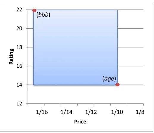
12 14 16 18 20 22

8 10 12 14 16 18

R

ating

Price

1/16 1/14 1/12 1/10 1/8

(age) (bbb)

Figure 3.7: Skyline Region

depict this in the shaded area. Any package that does not lie within this region can be immediately discarded. However, candidate packages may fall within this area and will need to be checked for membership in the skyline package.

Pruning and Early Termination

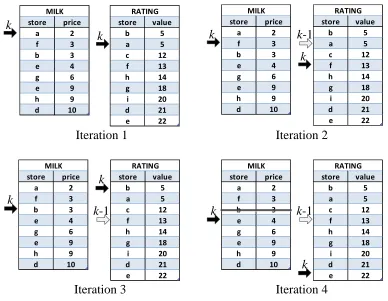
Since performing a Cartesian product is expensive and its output size to the number of package skylines ratio is very large, it is desirable to decrease this intermediate result. Therefore, we have to eliminate targets that cannot possibly be in the skyline set when packaged with any other available targets. While the naive approach would have to compose the packages and then perform a skyline to filter out unwanted tuples, our pruning technique offerslocal prunabilitythat prunes tuples, i.e., targets, from individual target qualifiers before we form the packages.

To illustrate the concept of local pruning, consider the milk and rating tables in Figure 3.6. We present in Figure 3.2.4 four iterations where each iteration indicates a new tuple being examined. As we look at each store in the milk table, we probe the

(37)

store value b 5 a 5 c 12 f 13 h 14 g 18 i 20 d 21 e 22 RATING store price a 2 f 3 b 3 e 4 g 6 e 9 h 9 d 10 MILK store value b 5 a 5 c 12 f 13 h 14 g 18 i 20 d 21 e 22 RATING store price a 2 f 3 b 3 e 4 g 6 e 9 h 9 d 10 MILK store value b 5 a 5 c 12 f 13 h 14 g 18 i 20 d 21 e 22 RATING store price a 2 f 3 b 3 e 4 g 6 e 9 h 9 d 10 MILK store price a 2 f 3 b 3 e 4 g 6 e 9 h 9 d 10 MILK store value b 5 a 5 c 12 f 13 h 14 g 18 i 20 d 21 e 22 RATING

Iteration 1 Iteration 2

Iteration 3 Iteration 4

k

k k

k k-1

k-1

k-1 k

k

Figure 3.8: Pruning Example

and probe the rating table again. We compare its value against the previous pointer, denoted as k−1. Since the current store is better than the previous store, we remove the pointer from store a and continue to the third iteration. As usual, the current tuple (b,3) is used to probe the rating table. In this case, the current pointer k (b,5) is worse than the previous pointer k−1 (f,13), and thus we prune the tuple (b,3). Because the current pointer that points to (f,13) is no better than the previous pointer, we save this pointer and examine the next tuple as shown in iteration 4.

The concept of local prunability is formalized in the following lemma.

Lemma 3.2.4 (Pruning) Let Tj[k] be the value of object k in table Tj, then ∀k ∈ Ti1, i ∈ [1, n], if ∃j ∈ [n+ 1, m] such that Tj[k−1] ≺ Tj[k], and Ti[k−1] Ti[k] then object k does not produce a package skyline and can be pruned from Ti.

(38)

Tj[k]Tj[k−1], objectk−1 dominatesk, thusk cannot be part of the package skyline.

Lemma 3.2.4 ensures that any combination where k appears is not a package skyline. If we denote the size of each table T as |T|, then for each tuple pruned in Ti, the size

of the resulting Cartesian product is reduce to |T1| × |T2| × · · · ×(|Ti| −1)× · · · × |Tn|.

To illustrate this, after tuple (b,3) is pruned in Figure 4, the Cartesian product size is reduced from 448 tuples to 392 tuples.

We define the previous object to be a pointer to the best last seen object and the pointer is updated when a better object is examined. In Lemma 3.2.4, we denote the current object as k and the previous object ask−1. If Lemma 3.2.4 is not satisfied, the pointer that once pointed tok−1 is updated to point to k.

To increase performance of our algorithm, we utilize the following early termination strategy for each resource.

Lemma 3.2.5 (Early Termination) If k is the current object in Ti and for all j ∈

[n+ 1, m], Tj[k] is the best in Tj, then stop examining Ti and continue to Ti+1, i+ 1≤n.

Proof Assume there exists an object k + 1 in Ti that has not been examined. Then Ti[k]Ti[k+ 1], and Tj[k]Tj[k+ 1]. IfTj[k+ 1]6=Tj[k], then Tj[k]≺Tj[k+ 1]. Then

for any object afterk, Ti[k]Ti[k+ 1]Ti[k+ 2]· · ·. Therefore, every object after k is

dominated.

Lemma 3.2.5 allows us to stop examining tuples in a given table when the best object is seen in the target descriptive tables , i.e., rating table. For example, in Figure 3.2.4, since b has the highest rating, we stop scanning the milk table once b is examined and prune all tuples below it. If a target qualifying table does not contain the best object from the target descriptive table, we choose the next best object such that the target qualifying table contains this object.

After pruning, our next phase is performing a Cartesian product. As the product is produced, if there exist any tuples that do not satisfy (local) hard constraints, we discard these. Figure 3.9 shows the resulting tables after pruning.

(39)

store price store price store price

a 2 g 5 e 3

b 3 a 7 b 4

b 10

MILK EGGS BREAD

Figure 3.9: Pruning and Early Termination Result

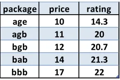
package price rating

age 10 14.3

agb 11 20

bgb 12 20.7

bab 14 21.3

bbb 17 22

Figure 3.10: Skyline Package Result

In Figure 3.9, a Cartesian product involving themilk,eggs, andbreadtables is performed to find (1) all packages and (2) total price. The intermediate result is then joined with the rating table to find the average rating. If there exists any tuples that do not satisfy (global) hard constraints, we discard these. A skyline algorithm is performed to remove any packages that are not skyline packages. The final skyline package set is shown in Figure 3.10.

Discussion

Now that we have provided a concrete example of the SkyPackage algorithm, we will now explain the pseudocode in Algorithm 4. Lines 1-3 of the algorithm explain some notations that are used within the algorithm. Once the query is issued, we examine each of the n tables (line 4) one row at time (line 6), keeping a pointer p that points to the

n+ 1 table that has the best value. With each iteration, we initialize ptr (line 5) to the first object in Ti mapped to Tn+1. Then we check whether Lemma 3.2.4 holds (line 7).

Lines 8-14 handles the case when two consecutive objects have the same value in Ti. In

this case, the tuple with the worse value in Tn+1 is pruned. Lines 15-17 are similar to

lines 8-14 except the equality checks are done on Tn+1 rather than Ti. That is if two

(40)

examining the current table when we access an object that has the lowest value in tn+1.

It can easily be showed that any tuple after this one cannot be in the skyline set. At this point, ptr can no longer be updated since any subsequent tuple will have a higher value in tn+1. If local constraints are given, we perform a check in line 19 to determine

whether the current tuple satisfies the constraints. If the current tuple is not satisfied, all tuples below and including this one are pruned. We then join the tables, removing any tuples that do not satisfy any global constraints. Lastly, any known skyline algorithm is performed.

Algorithm 4: SkyPackage

1: vk(i)← the value of object k in table i 2: k ← the current object (i.e., row) 3: ptr ← the best object

4: for all i∈[1, n] do

5: ptr←vx(n+ 1), x← first tuple ini 6: for all k ∈ti do

7: check whether Lemma 3.2.4 holds

8: if vk(i) =vk−1(i) then

9: if vk(n+ 1)> vk−1(n+ 1) then 10: prune (k, vk(i))

11: else

12: prune (k−1, vk−1(i)) 13: end if

14: end if

15: if vk(n+ 1) =vk−1(n+ 1) then

16: prune max{(k, vk(i)),(k−1, vk−1(i))} 17: end if

18: check whether Lemma 3.2.5 holds

19: check k against local constraints

20: end for 21: end for

22: cross product, remove tuples not satisfying global constraints

(41)

Chapter 4 Sesame Integration Framework

In this section, we present our implementation strategy for a loose integration with an open source RDF engine, Sesame 2, using a Web-based interface. We first provide an overview of Sesame’s architecture followed by the environment setup. Next, we discuss the client-server configuration used, and how we utilized Sesame’s server to query over HTTP.

4.1 Sesame

Sesame [14] is an open-source RDF database implemented in Java whose architecture allows for persistent storage of RDF data and querying of that data. For querying data, Sesame offers SPARQL and SeRQL (Sesame RDF Query Language) [13] querying and is extensible to other query languages.

We chose Sesame as our RDF engine for a number of reasons. First, since Sesame is a server-based application, it allowed us to store and query data on the Semantic Web remotely. Second, Sesame does not require a specific communication protocol or storage mechanism to be used.

Sesame implements a multi-layered architecture whose components are shown in Fig-ure 4.1. Since our framework is designed using HTTP, we exclude from our discussion the

Sail API,Rio, and SailRepository components. We next highlight the main components that are pertinent in our framework.

(42)

Figure 4.1: Sesame Components 1

The Repository API is a communication interface that offers a developer-friendly API for accessing (e.g., querying, manipulating, etc.) the data.

The HTTPRepository component is an implementation of the Repoistory API and offers a client-server communication over HTTP with the Sesame server.

TheHTTP Server component provides access to the repositories over HTTP using Java Servlets and requires a compatible Web container (e.g., Apache Tomcat).

4.2 Framework

In this section, we present an overview of our framework and a description of how we stored and retrieved the data.

The data that was used in the framework was the MovieLens2 _{dataset, which was}

converted to RDF format using the Jena API [15]. Its ontology is depicted in Figure 5.6. Figure 4.3 provides a high-level overview indicating the main components of our frame-work. We used a server with Linux and an Apache Tomcat Web container. A Web-based interface was designed to allow users to query a subset of the MovieLens dataset. Al-though any package-related query can be supported, for the purpose of this thesis, we chose to support a query of the following form.

Query 4.2.1 Find packages of n movies such that the average rating of all the movies is high, average release date is high, and each movie-rater has rated at least one of the

movies.

1_{Borrowed from}

http://www.openrdf.org/doc/sesame2/users/ch03.html

2

(43)

USER

MOVIE

string integer

hasRating hasUName

hasRated

string integer hasDate

hasMName

Figure 4.2: MovieLens Ontology

When the user provides preferences using the Web-based interface, the information is sent to the SPARQL adapter, which dynamically creates a SPARQL query. After the SPARQL query is executed and results of this query is available, the SkyP ackage

algorithm finds and presents the skyline package(s) that meet the user’s preferences.

4.2.1 Data Storage

One option of storing RDF triples is to store them in a text file. However, this is inefficient for large numbers of triples and a solution involving indexing (e.g., database management system) is more appropriate. Relational databases, such as MySQL and Oracle, can be used to store such data, but are usually not optimized for such. Databases that are optimized for storage of RDF triples are called triplestores.

Sesame triplestore stores RDF triples in a repository. Sesame abstracts from any particular storage mechanism allowing a variety of repositories to be handled, including RDF triplestores and relational databases. Sesame offers several repositories in which to store data and all differs in where the data is stored. Two popular repositories are

memory store andnativestore, corresponding to storage in-memory and on-disk,

(44)

Native

Store

Sesame

I/O

Server

Application

Client

Execute Query

Query Results

User submits preference(s)

Results Outputed

SkyPackage

SPARQL Adapter

Preferences sent to Adapter

Formatted Results

(45)

4.2.2 Data Retrieval

In order to retrieve data from Sesame’s repository, we devised a skyline package operator, whose ultimate goal is to form queries that when executed will construct the TQ and TD tables (§ 3.2.1). A description is given on how the queries for the TQ tables are constructed, followed by a similar description on how to construct the TD table.

We define SP(C, A, PF) as the skyline package operator that takes as arguments a list of constraintsC, a list of propertiesA, and a list of preferences P F. In addition, we assume that the following VPTs exist: vpt1, vpt2, . . . , vptm, vptm+1, vptn. Moreover, for

the purpose of illustration, we assume vpt1, . . . , vptm and vptm+1, . . . vptn are sufficient

to construct the TQ and TD tables, respectively. The arguments for the SP operator are defined as follows:

C = (c1, c2, . . . , cm), where ci are target qualifying constraints

A= (A1 = (a1, a2), A2 = (a01, a

0

2)), where ai and a0i are variables

A query is constructed for each target qualifying constraint (i.e.,mqueries) where the SELECT clause is formed by using variables in A1 (e.g., SELECT ?a1?a2). Within each

query, the constraint ci ∈C can be mapped to a FILTER clause or to a constraint in a

WHERE clause of a SPARQL query. In order to map the constraints to a WHERE clause, a target qualifying triple pattern is constructed (as described in§2.4) for each constraint. Assuming vpt1 contains data to which a constraint can be applied, the target qualifying

triple pattern is specified as (?var :vpt1 ci), where ?var is some variable. Moreover, the

remaining tablesvpt2. . . vptm are joined together and with the intermediate result of the

target qualifying triple pattern. A similar method can be applied if a FILTER clause is preferred. Instead of providing a constraint in the target qualifying triple pattern, a new variable is introduced, as in (?var :vpt1 ?constraint). This constraint variable is

then used in the FILTER clause along with the actual constraint to filter out unwanted results. An example FILTER clause is FILTER regex(?constraint, c1).

(46)

SELECT ?movieName ?rating

WHERE { ?user hasName: "user8". ?user hasRated: ?movie. ?movie hasMName: ?movieName. ?movie hasRating: ?rating. }

SELECT ?movieName ?rating

WHERE { ?user hasName: "user34". ?user hasRated: ?movie. ?movie hasMName: ?movieName. ?movie hasRating: ?rating. }

Figure 4.4: Queries to construct target qualifying tables

SELECT ?movieName ?date

WHERE { ?movie hasName: ?movieName. ?movie hasDate: ?date. }

Figure 4.5: Query to construct target descriptive table

following VPTs: hasName, hasRated, hasMName, hasRating. Since vpt1 is hasN ame,

we apply each constraint to this table by using a target qualifying triple pattern, such as (?user hasN ame“user8”). Therefore, given C and A1, the two queries in Figure 4.4 are

constructed, which produces the TQ tables

A similiar approach is used to form the TD table. Since no target qualifying con-straints are needed in this case, no FILTER condition is required and the only argument of interest isA2, which contains variables that will be listed in the SELECT clause. The

WHERE claused is formed by joiningvptm+1, . . . vptn. Continuing from the previous

ex-ample, we have the following VPTs: hasName, hasDate, andA2 = (?movieN ame,?date).

Therefore, the query in Figure 4.5 is constructed.

In order to retrieve data from Sesame’s repository, we implemented a server-side

SPARQL adapter whose primary task is issuing SPARQL queries and serves as an inter-mediary between Sesame and SkyP ackage. The adapter utilizes Sesame’s HTTPRep-soitory component to execute the three queries and to retrieve the results. The results of each query are then stored in a data structure for processing and sent to SkyP ackage

(47)

Chapter 5 Evaluation

In this chapter, we present the experiments conducted and the results of those experi-ments. We divided our experiments into two sections based on the data used, synthetic data and real data. We also provided an additional section that evaluates our storage model.

5.1 Overview

All experiments were conducted on a Linux machine with a 2.33GHz Intel Xeon processor and 40GB memory, and all algorithms were implemented in Java SE 6. All data used was converted to RDF format using the Jena API [15] and stored in Oracle Berkeley DB using B-tree indexes. All algorithms assumed data is initially stored on disk, and each tuple is brought into memory only when it is scanned.

We compared four algorithms,SkyP ackage,J CP S,SkyJ CP S, andRSJ F H (RDF

-SkyJoinWithFullHeader) [16]. During the skyline phase of each of these algorithms, we used the block-nested-loops (BN L) [10] algorithm. RSJ F H is similar to SkyJ CP S in that a skyline algorithm is performed before the Cartesian product. However, RSJ F H

is dependent upon the data being vertically partitioned, which increases the number of joins before the Cartesian product can be performed (see § 3.3). RSJ F H incorporates the join with knowledge of the skyline, thereby decreasing the number of tuples entering into the Cartesian product phase.

(48)

5.2 Synthetic Data

5.2.1 Dataset

Since we are unaware of any RDF data generators that allow generation of different data distributions, the data used in the evaluations were generated using a synthetic data generator [10]. The data generator produces relational data in different distributions, which was converted to RDF using the Jena API. We generated three types of data distributions: correlated, anti-correlated, and normal distributions. For each type of data distribution, we generated datasets of different sizes and dimensions.

5.2.2 Data Size Scalability

The first evaluation was performed to compare execution time among the three algorithms within the same package size using the three data distributions. The data consisted of triple sizes ranging from 450 to 635 and package sizes ranging from 2 to 5. While this may appear to be orders of magnitudes smaller than traditional evaluation corpora, it is important to note that the search space for package queries grows more aggressively than that of traditional pattern matching. We chose this triple size range to ensure that packages of different sizes can easily be compared and also to ensure that evaluation results would come in a reasonable time for larger package sizes. An increase in package size implies an increase in the number of tables, which also implies more Cartesian products. To ensure that the triple size remained approximately the same across different package sizes, we reduced the number of tuples in each table as the package size increased. Figure 5.1 shows the triple size and the number of tuples in each table for each package size as well as the approximate Cartesian product size.

(49)

Package

Size Triple Size

Tuples in each table

Approx Cartesian Product Size

635 35 52.5M

599 33 39M

545 30 24M

509 28 17M

455 25 9.7M

634 42 3.1M

604 40 2.5M

544 36 1.7M

499 33 1.2M

454 30 810,000

639 53 149,000

603 50 125,000

543 45 91,000

507 42 74,000

447 37 50,000

632 70 4,900

605 67 4,500

542 60 3,600

497 55 3,000

452 50 2,500

5

4

3

2

(50)

0.01 0.1 1

450 500 545 600 635

Exec u tion Ti m e ( sec ) Triple Size

Correlated (package size 2)

SkyPackage RSJFH SkyJCPS JCPS

0.01 0.1 1

450 500 545 600 635

Anti-Correlated (package size 2)

0.01 0.1 1

450 500 545 600 635

Normal (package size 2)

0.01 0.1 1 10

450 500 545 600 635

0.01 0.1 1 10

450 500 545 600 635

0.01 0.1 1 10

450 500 545 600 635

Exe cu tio n Tim e ( se c) Triple Size

(51)

0.01 0.1 1 10 100

450 500 545 600 635

0.01 0.1 1 10 100

450 500 545 600 635

Exe cu tio n Tim e ( se c) Triple Size

0.01 0.1 1 10 100

450 500 545 600 635

0.01 0.1 1 10 100 1000 10000

450 500 545 600 635

Exe cu tio n T im e ( se c) Triple Size

0.01 0.1 1 10 100 1000

450 500 545 600 635

0.01 0.1 1 10 100 1000

450 500 545 600 635

(52)

5.2.3 Package Size Scalability

Since the Cartesian product phase is likely to be the dominant cost in skyline package queries, it is important to analyze how the algorithms perform when the package size grows, which increases the input size of the Cartesian product phase. In Figure 5.4 we also show how the algorithms perform across packages of size 2 to 5 for the same triple size. For this experiment, we chose the largest triple size of 635, which yields the longest running time. For all package sizes, SkyJ CP S performs better than J CP S because of the initial skyline algorithm performed to reduce the input size of the Cartesian product phase. Unlike SkyP ackage, which uses early termination, SkyJ CP S has to examine every tuple and this adds to the total execution time. In addition, SkyP ackage utilizes a pruning technique that further reduces the Cartesian product’s input size. Note that there is a larger increase in execution time between package size 4 and package size 5 than there is between the other packages. This increase is merely due to the larger increase in size of the Cartesian product, as can be seen in Figure 5.1. Even though the tuples go through a pruning phase prior to entering the Cartesian product phase, the pruning power deteriorates as the package size increases, which is discussed in the next section.

RSJ F H outperformedSkyP ackagefor packages of size 5. We argue thatSkyP ackage

may perform slightly slower than RSJ F H on small datasets distributed among many tables. In this scenario, SkyP ackage has six tables to examine, while RSJ F H has only two tables. Evaluation results from the real datasets (later in this chapter) ensure us

that SkyP ackage significantly outperforms RSJ F H when the dataset is large and

dis-tributed among many tables. Due to the logarithmic scale used, it may seem that some of the algorithms have the same execution time as the triple size increases. This is not the case, and all algorithms’ execution increased as the data size increased.

5.2.4 Average Prunability

(53)

0.01 0.1 1 10 100

2 3 4 5

Execu ti on Ti m e (sec) Package Size

Anti-Correlated

0.01 0.1 1 10 100

2 3 4 5

Exec u tion Ti m e ( sec ) Package Size

Correlated

0.01 0.1 1 10 100

2 3 4 5

Execu ti on Ti m e (sec) Package Size

Normal

(54)

84 86 88 90 92 94

2 3 4 5

Per

ce

n

t

Pr

u

n

e

d

Package Size

Synthetic Data Prunability

SkyPackage

Figure 5.5: Prunability of Synthetic Data

of tuples increases as the package size grows. For example, a triple size of 635 for a package of size 2 consists of 140 tuples, whereas a package of size 5 has 175 tuples (a 25% increase). From our experiment, we discovered that as the number of tuples increases, the percentage of skyline packages decreases. Also, while performing SkyJ CP S, we found that the number of skyline tuples in the initial skyline phase increased as the number of tuples increased. Although the skyline size increased, the ratio between the skyline size and the number of tuples decreased, yielding a lower percentage. We argue that this is also the case with SkyP ackage.

5.3 MovieLens Dataset

The first real-world dataset evaluated was MovieLens1_{, which consisted of 10 million}

ratings and 10,000 movies.

1

SkyPackage: From Finding Items to Finding A Skyline of Packages on the Semantic Web.

ABSTRACT

DEDICATION

BIOGRAPHY

ACKNOWLEDGEMENTS

TABLE OF CONTENTS

LIST OF TABLES

LIST OF FIGURES

Chapter 1

Introduction

1.1

Thesis Motivation

1.2

Key Contributions

1.3

Thesis Organization

Chapter 2

Background and Related Work

2.1

Preference Queries

2.1.1

Skyline Queries

2.2

Semantic Web

2.2.1

RDF Data Model

2.2.2

SPARQL

2.3

Motivating Example

´

´

2.4

Problem Definition

2.5

Related Work

2.5.1

Historical Perspective

2.5.2

Single-relation Skyline Algorithms

2.5.3

Multi-relation Skyline Algorithms

2.5.4

Composite Top-

k

Algorithms

Chapter 3

Techniques for Evaluating Skyline

Packages

3.1

Algorithms for Package Skyline Queries over

Ver-tical Partitioned Tables

3.1.1

J CP S

Algorithm

3.1.2

RSJ F H

−

CP S

Algorithm



3.2

Algorithms for Package Skyline Queries over the

TDTQ Storage Model

3.2.1

The TDTQ Storage Model

3.2.2

Notations

3.2.3

SkyPackage Algorithm

Chapter 4

Sesame Integration Framework

4.1

Sesame

4.2

Framework

USER

MOVIE

4.2.1

Data Storage

_´