Fluctuation
Tests: How Reliable Are the Estimates
of
Mutation
Rates?
Frank
M.
StewartMathematics Department, Brown University, Providence, Rhode Island 02912
Manuscript received May 12, 1993 Accepted for publication April 25, 1994
ABSTRACT
Fifty one years ago, Luria and Delbrtick published in Genetics a paper that was to become a classic. In it they proved, beyond all reasonable doubt, that bacteria were mutating to phage resistance long before they could have encountered any bacteriophage. Luria and Delbriick also showed how the same experi- mental data could be used to estimate bacterial mutation rates. Since that time and in many different contexts the methods that they introduced have been used to estimate mutation rates. However, little seems to be known about the errors to be expected in such estimates. In what follows I examine how much uncertainty in the estimates is to be expected merely on the basis of the stochastic variability inherent in the sampling process. On the basis of this examination I question a few traditional ideas and conclude with some practical suggestions. The results were obtained by simulation. It is my hope that they may inspire others to provide a rigorous theoretical basis for such calculations.
I
N a typical fluctuation test, that is, an experiment of the kind introduced in LURIA and DELBR~~CK (1943), a number of cultures are grown up under conditions as nearly identical as possible. The cultures are started, each with a small inoculum of cells, assumed to be all of the same genotype. As the cells grow and divide some may mutate and give rise to clones of mutants. At the end of the growth period the cells are plated on some se- lective medium that will allow scoring the number of mutants that produce colonies of a particular pheno- type. One of the fluctuation analyst’s jobs is to tell the experimenter how to use his data to infer the rate of mutation to that phenotype. The goal of this study has been to try to find out what methods the analyst should recommend.The way to proceed is not obvious because, thanks to the growth of the mutants, the number of mutant colo- nies is not simply a function of the number of mutations. Understanding the significance of this fact was the key step in the research that led to the LUIUA and DELBR~CK
(1943) paper [FISCHER and LIPSON (1988)
p.
1451. LURIAand D E L B R ~ ~ C K were not able to find the relationship be- tween the number of mutations and the probability dis- tribution of the number of mutants. However, their ex- periments showed that the distribution has a variance that is much larger than its mean, which was enough to prove their main point. On the other hand, it meant that the mean could not provide a reliable method for esti- mating the mutation rate. Nevertheless, the formula they give for making the estimate is not as bad as it is sometimes painted.
In an earlier paper, STEWART et al. (1990), we de- scribed a general method for calculating the probability
Dedicated to MARY BRUCE DELBRUCK and our schoolmates
and teachers at the A.C.S.
Genetics 137: 1139-1146 (August, 1994)
distribution of the number of mutant colonies that will be observed in a fluctuation experiment. It assumes that the number of nonmutants is sufficiently large so that mutation can be treated as a stochastic process where: (i) the probability that a mutation will take place in the short interval between times t and t
+
d t is independent of what may happen at other times, and (ii) the condi- tional probability,p (
n I t ) , that a mutation will yield a count of n mutant colonies, given that it occurred at time t, depends on t , but not on what may happen at other times.Readers who wish to make calculations for themselves should be aware that the algorithm in STEWART et al.
(1990) is now obsolete. MA et al. (1992) describe an algorithm (that I will call “the MSS algorithm”) which is easy to understand and is manyfold faster than ours. The
MSS algorithm is also described in SARKAR et al. (1992). Of course, the actual distribution depends not only on the general assumptions (i) and (ii), but also on specific assumptions about the mutation process and the growth of the clones. For many experiments it is reasonable to assume that (a) the mutants grow at about the same rate as the original cells, (b) cell division is not synchronized and (c) the rate at which mutations occur is propor- tional to the number of cells present at that time.
In that case, the distribution depends on a single pa- rameter,
A,
the expected number of mutations, and is well approximated by the distribution worked out in LEAand C~ULSON (1949). In this report, I assume that the above conditions are satisfied and study only the LEA and
COULSON distribution. However, it would be of consider- able interest to investigate the robustness of estimates of A
1140 F. M. Stewart
The parameter
A
is not, in itself, of biological interest because the experimenter can vary it at will simply by changing the size of the culture vessel or the richness of the medium. What he really wants to know is notA,
but the mutation ratep.
This is the expected number of mutations divided by the number of cell divisions, i . e., p =A/(
nT - no), where no and nT are the initial and final population sizes. Since p is so easily calculated fromA this paper can concentrate on estimating the latter. We return to p only in the DISCUSSION where we take up accuracy and suggest a practical method for giving approximate confidence intervals for estimates of p. However, the essential formula, Equation 1, was ob-
tained by Monte Carlo methods and it is to be hoped that theorists will take an interest in the problem and provide more rigorous results.
This study deals with samples of samples, so care must be taken to avoid confusion of terms. I try to use real life terminology, but “simulated” is to be understood throughout. A single experiment studies a number of cultures, each of which yields a colony count. The num- ber of cultures in a given experiment is its sample size, denoted here, as in much of the literature, by
C.
Forsome purposes a number of experiments are considered together as a run consisting of a number of replications of the experiment.
A fluctuation experiment yields a set of C numbers, the colony counts for the C cultures. The experimenter calculates the value of some function of those numbers. The function is an estimatorand the value is the estimate of
A
given by that particular experiment.I have studied the behavior of five estimators that have been in common use. One of them, the maximum likeli- hood estimator, appears to be the best in all cases, but two of the others are quite satisfactory in some circumstances.
In the past, experimenters avoided maximum likeli- hood estimates because they were hard to calculate. There is no longer any need to avoid them. The MSS
algorithm described in h/iA et al. (1992) and SARKAR et al.
(1992) is easy to program. Using it, any computer with a mathematical coprocessor can calculate the probabil- ity distribution of colony counts, even up to 1500 or
2000, in a reasonably short time. The likelihood of the sample is a smooth function of A, and algorithms for finding the
A
that will maximize such a function are widely available.SIMULATED MATERIALS AND ACTUAL METHODS
The five estimators will be denoted by ‘A’s with sub- scripts that are intended to be mnemonic, as follows:
(1) The P O estimator is the value, A,,, that makes the expected number of cultureswithout mutants match the observed number. It is applicable only for small values of A, but when applicable it is the quickest and easiest method of estimation. (2) The LURIA and DELBRUCK es- timator is the value, A,,, = aN,, obtained by solving
Lum
and DELBR~CK (1943)’s Equation 8, i . e . , r = aNt ln(N,Ca),
where r is the average colony count in the sample, N, is the total number of cells in each culture, and a is the mutation rate. Historically minded readers may be interested to see how this much maligned esti- mator actually behaves. (3) The median estimator,AMED,
is the m that satisfies LEA and COULSON (1949)’s EQUA- TION 37: ( r o / m ) - In m = 1.24 where ro is the median sample count. (4) Similarly the LEA and COCJLSON esti- mator, A,,, is the m that satisfies their Equation 42:11.6
’
[
( q / m ) - ln m t 4.5+
2.02 = 0i= 1
1
where r, is the ith colony count. (5) The maximum like- lihood estimator,
A,,,
is adequately described in any number of texts.Some colleagues and I generated data by executing a computer program 16 times, four times for each of four sample sizes, namely 16, 32, 64 and 128, cultures per experiment. The program simulates six runs of 100 ex- periments, each run having a different value of A. In these executions the values were
A
= 0.5, 1.0, 2.0, 4.0, 8.0 and 16.0. Thus the data come from 9,600 simulated experiments with a total of 576,000 simulated cultures. One execution with a sample size of 16 had to be abandoned because in one of its experiments none ofthe cultures developed any mutants. The program is not designed to cope when the logarithm of the estimate is
--to.
The program was executed an additional time, with a different random seed, and that execution was used instead of the aborted one. The net effect is as if the single experiment had been replaced by another. Of course, such arbitrary action biases the result, but the effect of discarding one experiment out of 401 should be negligible.To generate the colony counts, the program uses the
MSS algorithm to fill an array cump [ 0 . .15 0 0 ] with the cumulative distribution function of the LEA and COULSON distribution. It then invokes the pseudo- random number generator ran1 of PRESS et al. (1988)
to get a value
rv,
0<
rv
< 1. The colony count is the smallest integer k such that r v<
cump[k] or, ifcump[1500] 5 rv, the colony count is set to the “jackpot value” 1501.
When the colony counts for a given experiment have been obtained, the program calculates from them the five different estimates for A and records the results.
RESULTS
When thinking about how to estimate the mutation rate, it is important to distinguish between two different
0.1% 1% 5% 25% 50% 75% 95% 99% 99.9%
A
Standard Deviations and %iles of the Normal Distribution0.1% 1% 5% 25% 50% 75% 95% 99% 99.9%
B Standard Deviations and %iles
of the Normal Distribution0.1% 1% 5% 25% 50% 75% 95% 99% 99.9%
c
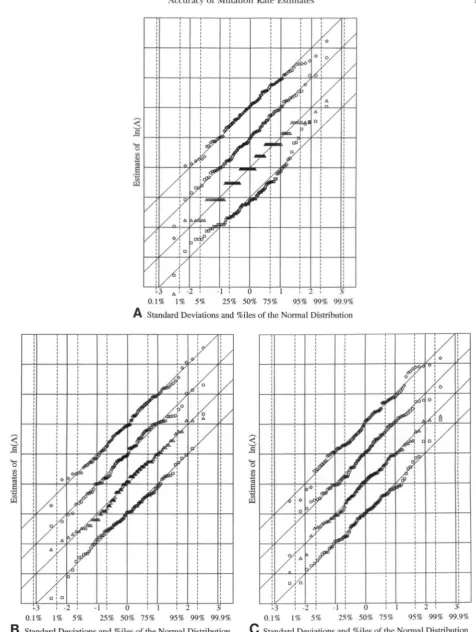
Standard Deviations and %iles of the Normal Distribution FIGURE 1.-The distribution of estimators for L compared with the normal distribution. (A and B) T h e estimators. Parameter values: C = 16 a n d A = 0.5 in A, C = 128 a n d A = 16.0 in B. Estimators:0,
IaD; A, I, (in A) or I,,,,, (in B); 0, L,& 0 , IW,.1142 F. M. Stewart
fixed
hESTIMATED
will vary from experiment to experiment so it is a random variable. The questions are: (1) ‘Which of the five suggested estimators should the experi- menter use?” and (2) ‘What does AESTIMATED tell us about A,,,?”In estimating the mutation rate, it is better to use a geometric rather than an arithmetic scale, in other words, to study the bias and variance of the logarithm of the rate rather than the mutation rate itself. For that reason, much of what follows will be concerned with a random variable L = ln(A,,,mT,D) or, when it is nec- essary to make distinctions among the estimators, with
L,, A,,,, L,,,, L,,, and L,,, these being the logarithms
The distribution of
L: Figure
1 presents typical graphs that show the distributions of L,, and L,,, to be quite close to normal. For each of the 100 replicates in the run there are four marked points, one for L,,,, one for L,, or L,,,, one for L,,,, and one for L,,. To begin with the estimates of, for example,&,
obtained in that run are sorted so that the first estimate is the smallest, the second is the next smallest, and so on. Then the sample is standardized by a linear transformation that makes its mean zero and its variance one. Lety n
be the value thus obtained from the nth estimate. Let x, be the expected value of the nth smallest observation in a ran- dom sample of size 100 drawn from a standardized nor- mal population. The estimate is plotted as the point(x,, y,)
.
To present four different estimators on a single graph, the y-scales for the different estimators are sepa- rated by one standard deviation.The plots to be shown in Figure 1, A and B, were chosen by lot from those with parameters at the extreme ends of the range being studied. For purposes of com- parison, Figure 1C shows what happens when four in- dependent random samples from a normal population are plotted in exactly the same manner. Similar plots using the estimates for
A
rather than its logarithm, L,showed a systematic curvature, particularly for the smaller sample sizes.
Although the distributions of L,,, L,, and L,,,, are not as close to normal as are those of LLkC and L,,, the agreement is close enough to indicate that means and variances will provide a sound basis for choosing among possible estimators.
The standard deviation
and
percentage points of&:
To give approximate confidence intervals for AACTUAL it will be necessary to give a formula, Equation 1, for cal- culating the standard deviation of L,, as a function of
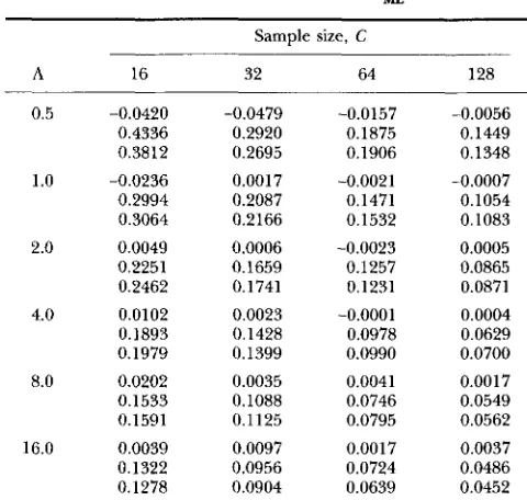
A,,,,. The data needed to derive the formula are given in Table 1. For this and all other tables, results for a given parameter set are grouped together so all runs consist of 400 replications.
Corresponding to each sample size, C, and expected number of mutations, A, Table 1 has three entries, the top two give the bias and standard deviation of L,, as Of ‘p09 ‘L&D? ‘MED, ‘L&, and ‘ML*
TABLE 1
Bias and s t a n d a r d deviation of L,
Sample size, C
A 16 32 64 128
0.5 -0.0420 -0.0479 -0.0157 -0.0056 0.4336 0.2920 0.1875 0.1449 0.3812 0.2695 0.1906 0.1348
1.0 -0.0236 0.0017 -0.0021 -0.0007 0.2994 0.2087 0.1471 0.1054 0.3064 0.2166 0.1532 0.1083
2.0 0.0049 0.0006 -0.0023 0.0005 0.2251 0.1659 0.1257 0.0865 0.2462 0.1741 0.1251 0.0871
4.0 0.0102 0.0023 -0.0001 0.0004 0.1893 0.1428 0.0978 0.0629 0.1979 0.1399 0.0990 0.0700 8.0 0.0202 0.0035 0.0041 0.0017 0.1533 0.1088 0.0746 0.0549 0.1591 0.1125 0.0795 0.0562
16.0 0.0039 0.0097 0.0017 0.0037 0.1322 0.0956 0.0724 0.0486 0.1278 0.0904 0.0639 0.0452
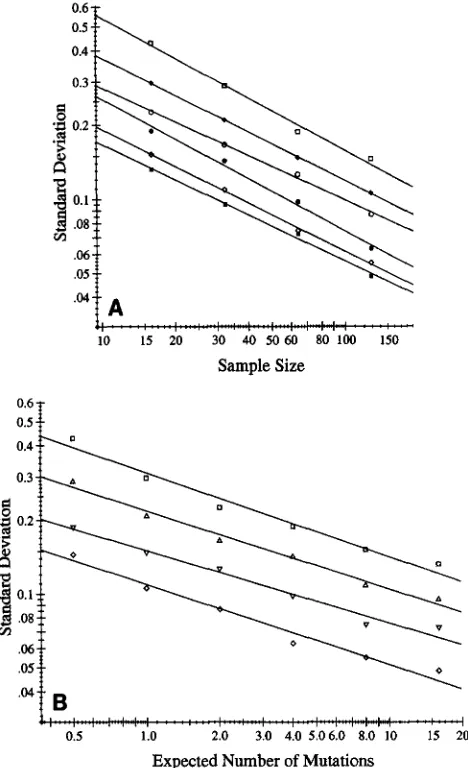
obtained from the simulations. The third entry is the estimate of the standard deviation given by Equation 1. The way the standard deviation of L,, varies with A
and C is shown in the log-log plots of Figure 2. In each part of the figure the values of the standard deviation as given in Table 1 are plotted as functions of one of the parameters, with different symbols distinguishing, in Figure 2A, the values for different sample sizes and, in Figure 2B, those for different values of
A.
The fact that the points lie nearly on straight lines implies that, a p proximately, the standard deviation is jointly propor- tional to powers of and the sample size. When regression coefficients are calculated from the data, the exponent for the sample size is very close to the theo- retical -% so the latter is used in the formula:s = 1.225A-0.315/flC (1)
where s is the predicted standard deviation of L,,, A is
AACTUAL,
and C is the sample size. The -0.315 is the average slope of the lines in Figure 2B and the constant of proportionality, 1.225, is chosen to give the best fit between Equation 1 and the observed standard deviations.The percentage points of the frequency distribution of L,, for the different sample sizes and values of A are given in Table 2. To make the various entries compa- rable the observed values have been standardized. The logarithm of A is subtracted from the observed percent- age point of L,, and the result is divided by the standard deviation calculated using Equation 1. Consider, for ex- ample, the 5% point for a sample size of 32 and A = 4. When the estimates from the run of 400 cultures were arranged in increasing order of L,,, the 20th and 21st
0.6 t
10 15 20 30 40 50 60 80 100 150
Sample Size
+”I I ;“I-+:: I
0.5 1.0 2.0 3.0 4.0 5.06.0 8.0 10 15 20
Expected Number of Mutations
FIGURE 2.-The standard deviation of
kL
as a function of the parameters. (A) As a function of the sample size, C.0, A = 0.5;
+,
A = 1.0; 0, A = 2.0; 0 , A = 4.0; 0 , A = 8.0;W, A = 16.0. (B) As a function of the expected number of mutations, A. 0, C = 16; A, C = 32; V, C = 64; 0 , C = 128.
of 4.0 gives -0.23679. The standard deviation is esti- mated using Equation 1: 1.225 X 4-0.315/fi =
0.13993. Finally, -0.23679/0.13993 = -1.692 and that is the value you will find in Table 2.
The other estimators: The other results from the simulations are summarized in Table 3. Unlike Table 1
it has two and not three entries for each (C, A) pair. Because none of these estimators is as satisfactory as the maximum likelihood estimator, I have not tried to find confidence intervals from them and so there will be no need for an approximation for the standard deviation. In Table 3, as in Table 1, the upper entry is the sample bias and the lower is the sample standard deviation.
Since the PO method is not much good when A is greater than one and the method of the median is prac- tically useless when A is less than two, the results for those two methods have been combined in a single table. In Table 3 entries for A = 0.5,l.O in the
h0
andLE,
columns, are for the PO method while entries forA
= 2.0, 4.0, 8.0, 16.0 are for the method of the median.DISCUSSION
Tables 1 and 2 show that the reliability of the estimates of L improves not only with increasing sample size, but also with increasing A. Since absolute errors in L trans- late immediately into relative errors in the mutation rate, p, regardless of the value of A, experimenters should set things up to make the expected number of mutations large. Of course, the larger
A
the more colo- nies there will be to count. Equation 1 might provide some guidance in weighing the gain in accuracy against the cost of increased counting.The “other” estimators: A glance at Tables 1 and 3 will confirm the idea that Equation 8 of
LURIA
and DWRUCK (1943) is not a good way to estimateA.
It should certainly not be used nowadays, but the tables show that it does not deserve all the abuse that it has received.LEA and COULSON (1949) say explicitly that the mean of a large sample will give no better estimate than one from a single observation and KOCH (1982) appears to believe much the same thing. Table 3 shows that this extreme mistrust of
A,,,
is by no means justified. In- spection of any row in the LURIA-DELBRUCK columns of Table 3 shows that increasing the sample size will im- prove the accuracy of the estimate. Doubling the sample size does not cut the standard deviation by a factor of~,
but when A 2 4 the standard deviation is cut by a factor of 1.25 or more.It is true that with small sample sizes and small values of A a few of the estimates gave a mutation rate an order of magnitude too high, but even there the great majority give at least a rough idea of its size. In the most favorable case considered here-sample size = 128 and A = l6-not one of the 400 estimates of the mutation rate was in error by as much as a factor of 1.6.
Except for small sample sizes, Table 3 confirms state- ments in LEA and C o u t s o ~ (1949), ARMITACE (1952) and KOZIOL (1991), who agree that, for A
<
1, A, is an en- tirely satisfactory estimator, just about as good asAML.
It has the great advantage that it does not depend on a s sumptions about the mutation and growth process. However, it should be kept in mind that, whenA
is small, good accuracy requires large sample sizes, whatever method is used.Because it is so easy to calculate,
A,,,
is convenient for quick estimates when optimal behavior is not re- quired. It might also serve as a starting point in the more computation intensive search forAM,.
The constants in LEA and COULSON (1949) ’s formulas were derived using values A = 4,6,8,13, 15, so it is not surprising that ALscc is seriously biased for smaller values
1144 F. M. Stewart
TABLE 2
Percentage points of L,
Sample size, C Sample size, C
A 16 32 64 128 A 16 32 64 128
2.5% 0.5 -2.368 -2.457 -2.113 -2.198 95.0% 0.5 1.519 1.405 1.567 1.636
1.0 -2.035 -2.051 -1.988 -1.960 1.0 1.478 1.422 1.559 1.512 2.0 -1.792 -1.809 -2.010 -2.269 2.0 1.535 1.536 1.578 1.550 4.0 -1.817 -2.085 -1.904 -1.660 4.0 1.602 1.635 1.686 1.523 8.0 -1.591 -1.815 -1.824 -2.014 8.0 1.753 1.594 1.640 1.620 16.0 -1.859 -1.960 -2.224 -1.902 16.0 1.753 1.938 1.838 1.879
5.0% 0.5 -2.136 -2.038 -1.732 -2.006 97.5% 0.5 1.746 1.832 1.847 1.970
1.0 -1.680 -1.687 -1.598 -1.671 1.0 1.993 1.756 1.758 1.709 2.0 -1.528 -1.532 -1.684 -1.597 2.0 1.756 1.700 1.982 1.951 4.0 -1.606 -1.692 -1.592 -1.427 4.0 1.750 1.972 2.007 1.741 8.0 -1.384 -1.546 -1.457 -1.581 8.0 1.948 1.897 1.936 2.022 16.0 -1.663 -1.693 -1.829 -1.583 16.0 2.085 2.149 2.194 2.228
TABLE 3
Biases and standard deviations
Lpo and
hED
sample sizes L,,, sample sizes L,, sample sizesA 16 32 64 128 16 32 64 128 16 32 64 128
0.5 -0.0441 -0.0480 -0.0172 -0.0048 0.4697 0.4343 0.3342 0.3441 0.4156 0.3988 0.4114 0.4157 0.4431 0.2994 0.1889 0.1469 0.9000 0.8444 0.6604 0.6416 0.4965 0.4400 0.4320 0.4273 1.0 0.0066 0.0074 -0.0002 0.0003 0.3880 0.3980 0.3181 0.3202 0.2006 0.2218 0.2159 0.2197 0.4079 0.2390 0.1535 0.1182 0.7746 0.7312 0.6236 0.5332 0.3203 0.2806 0.2525 0.2369
0.2732 0.2090 0.1576 0.1176 0.7036 0.6007 0.5519 0.4124 0.2397 0.1922 0.1600 0.1333 4.0 0.0221 0.0023 0.0062 0.0096 0.3220 0.2826 0.2257 0.1645 0.0448 0.0454 0.0455 0.0460 0.2452 0.1822 0.1232 0.0800 0.6179 0.4964 0.4047 0.3003 0.2040 0.1523 0.1048 0.0784 8.0 0.0315 0.0164 0.0180 0.0149 0.3093 0.2043 0.1631 0.0810 0.0330 0.0140 0.0192 0.0178 0.2051 0.1377 0.0997 0.0737 0.5356 0.3947 0,2909 0.1908 0.1673 0.1169 0.0815 0.0588 16.0 0.0211 0.0264 0.0177 0.0179 0.2255 0.1656 0.0824 0.0155 0.0015 0.0109 0.0022 0.0056 0.1793 0.1345 0.1002 0.0704 0.3949 0.2999 0,1991 0.1244 0.1396 0.1023 0.0782 0.0531 2.0 -0.0001 0.0028 -0.0059 -0.0090 0.3850 0.3067 0.3066 0.2365 0.1071 0.1057 0.1024 0.1061
to be the method of choice were it not for the fact that calculating the maximum likelihood estimator is no longer an arduous chore.
Confidence intervals: To calculate a 95% confidence interval we need formulas for the 2.5 and 97.5% percent points of the distribution. Table
2
shows the 2.5 and 97.5% percent points of the simulated data after nor- malization as described in the RESULTS. For a normal dis- tribution these values would be k1.960.There may be some asymmetry and a directional trend in Table 2. I believe these effects are real, but have been unable to find any measure of departure from normal distributions with standard deviations calculated by Equation 1 that is statistically significant. Until further analysis provides a reliable way to quan- ti@ what trends there may be, I see no choice but to ignore them. It turns out that, over all, the confidence levels calculated this way seem to be surprisingly reliable.
If one assumes that L,, is approximately normally dis- tributed with mean ln(h) and standard deviation, s,
given by Equation 1, one would expect that about 95% of the estimates would lie within a distance of 1.960s of l n ( h )
.
In other words, since 1.960 X 1.225 = 2.401,about 95% of the estimates L,, = ln(A,,,~m,) will satisfy the inequalities
2.401e-0.315L 2.401e-0.315L
L -
f l c
<&,<L+f l c
(2)
where C is the sample size, and L = ln(A,,,)
.
To get a confidence interval you must substitute into this formula,
(2),
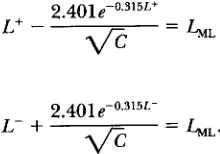
the value of L,, obtained from the experiment and solve the resulting inequalities. In other words, the confidence interval is the set of those L that satisfy L- < L<
L+ where L- and L+ are defined as the solutions of the equations2.401~-0.315L+
L+
-
= L M Ld-"
andL-
+
2.401~-0.315L- = L M L '
Accuracy of Mutation Rate Estimates
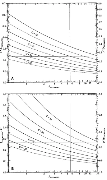
FIGURE 3.-Solid lines 95% and dotted lines 90% confidence factors for p. (A) Upper factors; (B) lower factors.
Since the inoculum of cells with which the cultures In(AEsT,mTED), are initiated is usually small compared to the final
population size, nT, assume, as is customary, that F = A A C T d n T and let F E S T I ~ T E D - A E S T I w T E d n T
be the value of p estimated from the experiment. If A' = eL+ then the upper end of the confidence interval for k , call it p', is A i / n T and, since
LL
=A+ eLt e ( L + - L ~ ~ ) e L ~ ~
P+
= - - - " -- nT nT n T
e ( L + - L ~ ~ ) A
-
EsTlmTED = e ( ~ + - L ~ ~ . )- FESTIMATED
9
1146 F. M. Stewart
In other words, the upper bound for p is obtained by multiplying the estimated value of p by a confidence factor e ( L + - L M L ) .
A similar argument will show that
p - = e - ( L ~ ~ - I . - )
PESTIMATED (5)
is the lower bound of the confidence interval for p. The solid lines in Figure 3A are plots of (L’ - LML)
as a function of
AESTIMATED,
using the linear scales that appear on the left-hand sides of the vertical lines. On the right-hand sides are logarithmic scales that give the corresponding values of eL+-LM1.. The upper bound for p is obtained by multiplying the experimental value, pESTIMATED, by the factor read from right-hand scale. Figure 3B is like Figure 3A except that it gives values for calculating the lower bounds.For example, suppose a fluctuation experiment with 32
cultures, each growing up to a population of approxi- mately 6.3 X lo8 cells, has yielded a maximum likelihood estimate of A = 5.6 so hsTIMATED = 5.6/6.3 X lo8 = 8.9 X lo-’. In Figure 3A a vertical line has been drawn at
A E s T I ~ T E D = 5.6. This meets the 95% confidence line at an upper confidence factor of 1.259. (Beware of optical illu- sions when drawing such lines by hand.) Thus the 95% upper bound for p is 1.259 X 8.9 X lo-’
-
1.12 Xlo-’.
Similarly from Figure 3B one gets a lower confidence factor of 0.764. Since 0.764 X 8.9 X
lo-’
-
6.8 X lo-’,one might say, with approximately 95% confidence, that
6.8 X lo-’ < p
<
1.12 X (6)The dotted lines in Figure 3 give the 90% confidence factors in the same way that the solid lines give the 95% factors.
In spite of the uncertainty suggested by Table
2,
Equa- tions 4 and 5 appear to fit the simulations remarkably well. Of 9,600 90% confidence intervals calculated from them 8,654, i. e . , 90.1%,
include the true value. The corresponding figure for the 95% intervals is 9,112,i. e . , 94.9%.
Caveat: All of the simulated samples were drawn from a LEX and COULSON distribution. If the actual mutation process is not close to their model there is no reason to expect that numbers that appear in the formulas will be correct. Much more simulation will be necessary before the conclusions of this study can be applied to such pro- cesses. Moreover, a more theoretical and rigorous study of the estimation procedures is much to be desired.
SUMMARY
This report studies maximum likelihood estimation of mutation rates from data obtained in fluctuation experi-
ments. Extensive simulations show that the behavior of the maximum likelihood estimator is sufficiently regular that it is possible to give approximate confidence inter- vals for the mutation rate. Graphs are provided by which 90 and 95% confidence intervals can be calculated for a wide range of experimental parameters. Since the maximum likelihood estimate is now easy to calculate and is better than any of the other estimates suggested, it should probably be used for all serious work. The highest accuracy will be obtained when the expected number of mutations is as large as experimental conditions permit. The simulations show that the original averaging method used by LURIA and DELBRUCK is somewhat better than has often been suggested. When the expected num- ber of mutations is small, estimation by the number of cultures without mutants is almost as reliable as the maximum likelihood method, but low expected num- bers should be avoided when possible. For small values of the expected number LEX and COULSON’S method is seriously biased, but for larger values it is almost as ac- curate as maximum likelihood.
I am most grateful to two reviewers for careful and very helpful reviews of earlier versions of this paper. I also want to thank A N D Y BROWDER, PHYLLIS HUDECK, MIKE ROSEN and JOE SILVERMAN, who used their computers to get the data on which this study is based.
LITERATURE CITED
ARMITAGE, P., 1952 The statistical theory of bacterial populations sub- ject to mutation. J. Roy. Stat. SOC. B 1 4 1-40.
FISCHER, E. P., and C. LIPSON, 1988 T h i n k i n g About Science. W. W. Norton, New York.
KOCH, A. L., 1982 Mutation and growth rates from Luria-Delbnick fluctuation tests. Mutat. Res. 9 5 129-143.
KOZIOL, J. A,, 1991 A note on efficient estimation of mutation rates using Luria-Delbrcck fluctuation analysis. Mutat. Res. 249:
LEA, E. A,, and D. E. COUWN, 1949 The distribution of the numbers of mutants in bacterial populations. J. Genet. 49: 264-285. LURIA, S. E., and M. DELBRUCK, 1943 Mutations of bacteria from virus
sensitivity to virus resistance. Genetics 28: 491-511.
MA, W. T., Gv. H. SANDRI and S. SARKAR, 1992 Analysis of the Luria- Delbrcck distribution using discrete convolution powers. J. Appl. Prob. 2 9 255-267.
PRESS, W. H., B. P. FLANNERY, S. A. TEUKOLSKY and W. T. VETTERLING, 1988 Numen’cal Recipes in C. Cambridge University Press, New York.
SARKAR, S., 1991 Haldane’s solution of the Luria-Delbnick distribu- tion. Genetics 127: 257-261.
SARKAR, S., W. T. MA and Gv. H. SANDRI, 1992 O n fluctuation analysis: a new, simple and efficient method for computing the expected number of bacterial mutants. Genetica 8 5 173-179.
STEWART, F. M., D. M. GORDON and B. R. LEVIN, 1990 Fluctuation analysis: the probability distribution of the number of mutants under different conditions. Genetics 1 2 4 175-185.
275-280.