ABSTRACT
TIDEMANN-MILLER, BETH A. Statistical Modeling of Multivariate Functional Data that Exhibit Complex Correlation Structures. (Under the direction of Brian Reich and Ana-Maria Staicu.)
Due to the large size of modern data sets, there is an ever-increasing need for computationally efficient inferential methods designed for realistic models of large observed functional data sets. The first part of this dissertation introduces an inno-vative modeling framework for the analysis of multivariate functional data, where each individual functional component exhibits multilevel and spatial structures. The proposed methodology uses a functional principal components based approach for multivariate functional data, which has important advantages in the dimensionality reduction of the data and brings considerable computational savings. Moreover, our approach quantifies the spatial auto- and cross-correlation between units at the low-est level of the hierarchy. The proposed procedure is illustrated through simulation studies and data from a colon carcinogenesis experimental study.
© Copyright 2014 by Beth A. Tidemann-Miller
Statistical Modeling of Multivariate Functional Data that Exhibit Complex Correlation Structures
by
Beth A. Tidemann-Miller
A dissertation submitted to the Graduate Faculty of North Carolina State University
in partial fulfillment of the requirements for the Degree of
Doctor of Philosophy
Statistics
Raleigh, North Carolina
2014
APPROVED BY:
Brian Reich
Co-chair of Advisory Committee
Ana-Maria Staicu
Co-chair of Advisory Committee
Marie Davidian Arnab Maity
DEDICATION
BIOGRAPHY
ACKNOWLEDGEMENTS
It is with the deepest gratitude that I acknowledge several key individuals who have accompanied me on this educational journey. Primarily, I wish to thank my co-advisors, Drs. Ana-Maria Staicu and Brian Reich, for their dedication to helping me see this work through to completion. They have molded me into a more thoughtful, critical, insightful, and technically sound statistician, and I will benefit from their in-struction for years to come. To my committee members, Drs. Arnab Maity, Sukanta Basu, and Marie Davidian, I extend my appreciation for the valuable input they have provided for the research contained in this dissertation. I would like to acknowledge Dr. Davidian in particular for her support throughout my graduate school career. The chance to work on her training grant was the deciding factor in my choice of graduate programs, and she has shown continued commitment to my professional development through financial assistance and mentorship. I also would like to ex-press my gratefulness to Dr. Montserrat Fuentes for her many kindnesses and sound professional guidance. To all of my professors at NCSU, I extend many thanks.
The members of the astounding departmental staff at NCSU have been my life-lines. There is no adequate way in which to express exactly how much dear, sweet, Alison McCoy has meant to me throughout this process. Her encouragement, hugs, smiles, and love always carried me through the rough patches, and I am eternally grateful for her friendship. Also, I am convinced my simulations would still be run-ning if it weren’t for the help of Terry Byron and Chris Waddell who are always willing to share their invaluable IT knowledge and accommodate my many and var-ied requests for assistance.
My success in graduate school is due in large part to the solid background in Mathematics and Statistics that I received at the University of Nebraska-Lincoln. For their gentle nudges that led me to be a Math major and to explore Statistics, I thank Drs. Mohammad Rammaha and Gordon Woodward. For the high quality statistical instruction that prepared me well for graduate school, I thank Drs. Erin Blankenship, Walter Stroup, Tisha Hooks, Jacqueline Wroughton, and Chad Brassil. Drs. Blanken-ship and Brassil served as my undergraduate co-advisors, and it was under their instruction that I successfully completed my undergraduate honors thesis.
To my family and friends: you have continually given me your love, support, encouragement, patience, understanding, and kindness throughout this journey. To Mom and Dad, thank you for teaching me to be inquisitive, respectful, and persever-ant, to do my best in all things, and to make school a priority. Darcia and Jeremy, as your little sister I have always looked up to you and had the privilege of following your example. Thank you for demonstrating such dedication to academics, motivat-ing me to challenge myself, and believmotivat-ing in my potential from day one.
TABLE OF CONTENTS
LIST OF TABLES . . . viii
LIST OF FIGURES . . . ix
Chapter 1 Introduction . . . 1
1.1 What is functional data analysis? . . . 1
1.2 Smoothing . . . 3
1.2.1 Basis Expansions . . . 4
1.2.2 Roughness Penalties . . . 6
1.2.3 Kernel Smoothing . . . 7
1.3 Functional Principal Components Analysis . . . 9
Chapter 2 Modeling Multivariate Spatial Functional Data . . . 12
2.1 Background . . . 12
2.2 Model for multivariate functional response . . . 14
2.2.1 Model Assumptions . . . 15
2.2.2 Bivariate Matérn structure for spatial covariance . . . 16
2.2.3 Modeling of functional processes . . . 16
2.2.4 Notation for balanced design . . . 17
2.3 Estimation . . . 18
2.3.1 Spatial covariance estimation . . . 19
2.3.2 Raw functional covariance estimates . . . 22
2.3.3 Multivariate multilevel FPCA . . . 23
2.3.4 Estimate group mean functions . . . 24
2.4 Simulations . . . 25
2.4.1 Data generation . . . 25
2.4.2 Computational Details . . . 26
2.4.3 Results . . . 27
2.5 Colon carcinogenesis study; joint analysis of apoptosis and p27 . . . 30
2.5.1 Results from FULL Model . . . 33
Chapter 3 Modeling Multivariate Mixed-Response Functional Data . . . 36
3.1 Background . . . 36
3.2 Model . . . 38
3.2.1 General Framework . . . 38
3.2.2 Predetermined bases . . . 40
3.2.3 Data-driven bases . . . 40
3.2.4 Prior Specification . . . 43
3.4 Simulations . . . 45
3.4.1 Data generation . . . 45
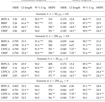
3.4.2 Models and metrics for comparison . . . 45
3.4.3 Results . . . 47
3.5 Periodontal Data Application . . . 48
Chapter 4 Conclusion . . . 55
References . . . 58
Appendices . . . 66
Appendix A Additional details for Chapter 2 . . . 67
A.1 Colon carcinogenesis study; additional results . . . 67
A.1.1 Prediction . . . 69
A.2 Simulations: Scenarios 5 & 6 . . . 71
A.3 Weighted least squares for initial values . . . 74
A.4 Additional simulation results for Scenarios 1-4 . . . 74
Appendix B Additional details for Chapter 3 . . . 80
B.1 Approximating Smooth Covariance . . . 80
B.2 Latent Cross Covariance Estimator . . . 81
B.3 Derivations of Posteriors . . . 82
B.3.1 Random effects . . . 82
B.3.2 Random effects precision matrix . . . 83
B.3.3 Fixed effects . . . 84
LIST OF TABLES
Table 2.1 Specifications for Scenarios 1-4 . . . 25
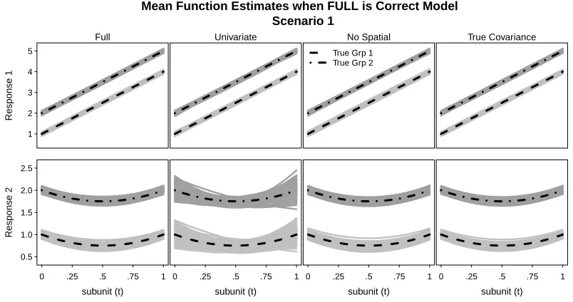
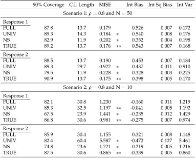
Table 2.2 Mean function estimation comparisons for Scenarios 1 & 2 when FULL is generating model . . . 29
Table 3.1 Simulation Results . . . 47
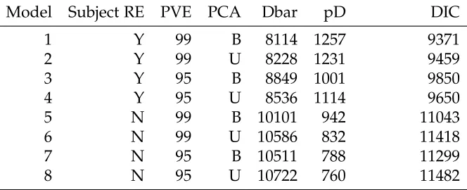
Table 3.2 Model comparisons for the periodontal data application . . . 50
Table A.1 Prediction and Cross Validation . . . 70
Table A.2 Model comparisons for Scenarios 5 and 6 . . . 72
Table A.3 Mean function estimation comparisons for Scenario 3 when FULL is generating model . . . 75
LIST OF FIGURES
Figure 2.1 Group mean functions when FULL is the generating model with
ρ =0.8 and N=50 (Scenario 1) . . . 28
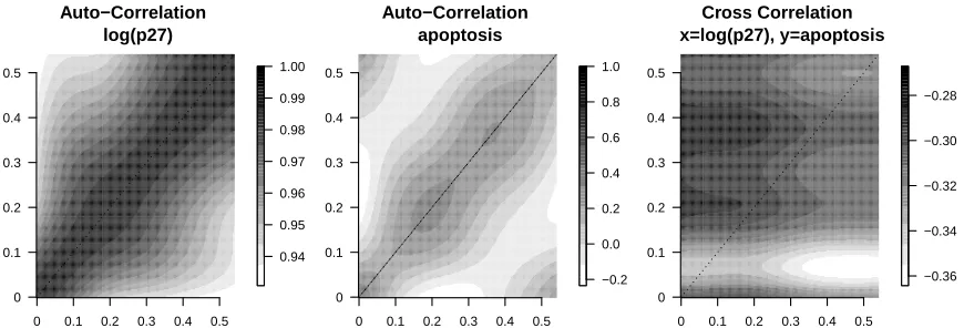
Figure 2.2 Colon Crypt Depiction . . . 30 Figure 2.3 Image of marginal auto- and cross-correlation matrices for a crypt.
Lines have been added to the diagonals. . . 34 Figure 2.4 Diet mean estimates using FULL. . . 34
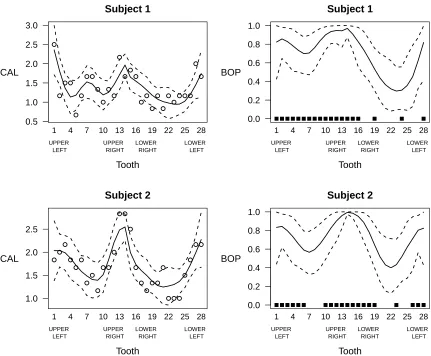
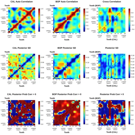
Figure 3.1 Posterior medians and 95% posterior intervals of the subject-specific covariate coefficients by response. . . 51 Figure 3.2 Fitted values for two individuals from the periodontal study. . . 52 Figure 3.3 Posterior summaries of the within-response and
between-response correlation structures for any two teeth . . . 53
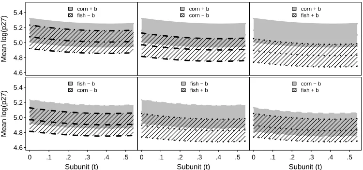
Figure A.1 Pairwise diet comparisons of mean log(p27) estimates and 95% GLS confidence intervals for the FULL method. . . 68 Figure A.2 Pairwise diet comparisons of mean apoptosis estimates and 95%
GLS confidence intervals for the FULL method. . . 68 Figure A.3 Estimated Eigenfunctions . . . 69 Figure A.4 Diet mean functions for each response from all models. . . 71 Figure A.5 Group mean functions when NS is the generating model with N =
10 (Scenario 5) . . . 73 Figure A.6 Group mean functions when COMPLEX is the generating model
with N=10 (Scenario 6). . . 73 Figure A.7 Group mean functions when FULL is the generating model with
ρ =0.8 and N=10 (Scenario 2). . . 76
Figure A.8 Group mean functions when FULL is the generating model with
ρ =0.2 and N=50 (Scenario 3) . . . 76
Figure A.9 Group mean functions when FULL is the generating model with
ρ =0.2 and N=10 (Scenario 4) . . . 77
Figure A.10 Matérn correlation function estimates . . . 77 Figure A.11 Eigenfunctions obtained by fitting FULL for level 1 functional
pro-cess when FULL is the generating model withρ=0.8 and N =50
(Scenario 1). . . 78 Figure A.12 Eigenfunctions obtained by fitting FULL for level 2 functional
pro-cess when FULL is the generating model withρ=0.8 and N =50
(Scenario 1) . . . 78 Figure A.13 Eigenfunctions obtained by fitting FULL for level 1 functional
pro-cess when FULL is the generating model withρ=0.8 and N =10
Figure A.14 Eigenfunctions obtained by fitting FULL for level 2 functional pro-cess when FULL is the generating model withρ=0.8 and N =10
CHAPTER
1
Introduction
1.1
What is functional data analysis?
The area of Statistics known as functional data analysis (FDA) has undergone many methodological developments in the past two decades and is still experiencing intense growth. Many types of electronic devices can now observe functions at very fine increments and have become ubiquitous in a wide variety of disciplines. Such a rapid advancement of technology in recent years has elevated the level of interest in FDA as researchers seek innovative ways of handling large and increasingly complex data that come in the form of functions.
Unlike other statistical frameworks (e.g. longitudinal, multivariate, or time-series), FDA views an observed function as a single (functional) datum. For example, con-sider an electrocardiogram (ECG) machine that monitors the electrical activity of a patient’s heart every fraction of a second for one hour. For the purposes of FDA, the entire function of ECG observations for the hour comprise one functional datum, contrary to more traditional approaches where the value of the ECG at a single time point would be an individual datum.
functional data analysis: methods and case studies (Ramsay and Silverman 2002) helped to unify FDA methods to form a statistical sub-discipline. FDA was justing start-ing to gain momentum within the statistical community around the time the second edition of Functional Data Analysis was published (2005) and also the well regarded FDA monograph of Ferraty and Vieu (2006) appeared. Also around this time, spe-cial issues of several journals were devoted to exploring FDA in more depth, such as bridging the gap between longitudinal data analysis and FDA (see Davidian M. and Wang (2004); Rice (2004)), modeling functional data (see Valderrama (2007)), and other topics (see Gonzalez-Manteiga and Vieu (2007)).
Although FDA is a relatively new area of statistical analysis, methodology has developed to such an extent that topics of major interest such as regression, clas-sification, and prediction, to name a few, have existing analogues within FDA. For example, functional linear regression incorporates a functional predictor to model ei-ther a scalar response (Cardot et al. 2007; Crambes et al. 2009; Ferraty and Vieu 2002; James 2002) or a functional response (James et al. 2009; Liang and Zeger 1986; Wu et al. 1998; Yao et al. 2005b). Importantly, the goals of FDA align with those of any other area of Statistics, for instance, describing central tendency and variation, and forming parsimonious models. Unique to FDA is the ability to use derivatives of the curves to inform an analysis. Sometimes, trends in the derivative itself are of interest. A good example of this comes from a growth curve study described in Chapter 1 of Ramsay and Silverman (2005) in which profiles of girls’ height were collected from childhood to adolescence. For this study, one might be interested the speed (first derivative) and acceleration (second derivative) of the height profiles.
In FDA a function is considered as having an infinite-dimensional domain, al-though in reality only a finite number of realizations of the function can be collected. Many methods in FDA assume that the functional data are observed densely over the domain, meaning values of the curve are evaluated frequently. When data is observed sparsely, methods for densely observed functional data may no longer be applicable. For simplicity we mainly focus our attention to the densely observed case and only briefly touch upon methods for sparse data.
The goal of this introduction is to provide a primer for the content that follows in subsequent chapters. It is meant to introduce the reader to the lens through which FDA approaches data analysis and to familiarize the reader with concepts that are both common within FDA and also recurrent throughout the methodologies we pro-pose later on. The information presented in this introduction is largely compiled from Ramsay and Silverman (2002), Ramsay and Silverman (2005), and the collection of works found in Ferraty and Romain (2011), and we suggest that the reader consult these or other texts for a more comprehensive review of FDA.
1.2
Smoothing
The concept of smoothness is an integral part of FDA since it is assumed that functional data emanate from a smooth underlying process. Saying a function is smooth usually means that one or more derivatives exist (Ramsay and Silverman (2005), Ch. 3). More simply, it means the function is devoid of abrupt changes and smoothly transitions from one value to the next.
To further understand the meaning of smooth functions, consider the functional datum Y(t) collected at corresponding evaluation points t = t1, . . . ,tL within some
intervalT. We can view the datum as L realizations (observed with or without error) of a smooth function s(t), where the underlying function s(t) is also defined for t ∈ T. When the datum is observed without error, we can use the modelY(t) = s(t), and recovering the underlying functions(t) is called interpolation. More commonly, the datum suffers from observational error, making the observed curve rough or wiggly, and an appropriate model is Y(t) = s(t) +e(t) wheree(t) is a random error
process. In this case, recovering s(t) is known as smoothing.
researcher to evaluate s(t) at any t ∈ T, not just at the evaluation points t`, ` = 1, . . . , L, where Y(t) is observed. How dense the evaluation points t` are within the domain T along with the curvature of the underlying function determine what is known as the resolution of the curve.
If the resolution of the curve is low, meaning the observations are too sparsely observed to adequately capture the features of the underlying process, then smooth-ing individual curves may not be appropriate. Given a sample of curves Yi(ti`), i =1, . . . , N, where each curve is observed at Li evaluation pointsti`, one can smooth each curve by borrowing information across curves. Methods for this sparse case include mixed effects modeling and local smoothing, among others; we direct the interested reader to James (2011) for an excellent review of methods for sparse data related to principal components, clustering, classification, and regression.
Smoothing is primarily achieved using 1) global smoothing methods such as basis expansions with or without roughness penalties, and 2) local smoothing methods such as kernel smoothers. The basis expansion method uses a linear combination of basis functions to represent a smooth function. This method is described in Section 1.2.1 with particular attention given to B-splines (de Boor 1978) which Ullah and Finch (2013) found to be the most popular smoothing method implemented within the FDA literature. Basis functions can be used in conjunction with a roughness penalty approach finds the function that fits the data well but also does not exhibit too much local variation (Section 1.2.2). Kernel smoothing is described in Section 1.2.3.
1.2.1 Basis Expansions
Expressing a smooth function as an expansion of basis functions is commonplace within FDA and appears frequently in the methodologies presented in Chapters 2 and 3. The basis expansion approach has several uses such as smoothing the raw data, representing the data at any location in the domain (regardless of whether a function value was measured at that point), and unifying a sample of curves that were observed for different evaluation points in the domain.
polynomial function f(t) of degree K−1 can be represented by a linear combination of these basis functions, that is, f(t) =∑Kk=1βkt(K−1). In general, let f(t)be a smooth function and let {φk(t) : k ≥ 1} be a set of basis functions (considered known) for t ∈ T. Using a basis expansion, the function f(t)is approximated by
f(t) ≈ K
∑
k=1
βkφk(t), (1.1)
where the parameter K is the number of basis functions included in the expansion and the parameters βk are unknown but fixed coefficients that can be estimated through regression methods such as least squares.
Given that an appropriate basis system is chosen, the quality of the approximation in (1.1) depends on the value of K. For observed function values f(t`), `=1, . . . , L, it is possible for the basis expansion to interpolate the values f(t`)exactly if the number of basis functions is chosen to be equal to the number of evaluation points, that is, by setting K=L (Ramsay and Silverman 2005). Even though specifying a large number of basis functions might offer an excellent fit to the data, overfitting is a pitfall one should avoid. In practice, the number of basis functions should be much smaller than the number of evaluation points but still large enough to provide a good fit. Indeed, the goal of using a basis function expansion is to specify a basis system that fits the data well for a relatively small value of K.
Since the set of basis functions is considered known in advance (pre-determined), it is important that the choice of basis system coincides with the features of the data and the goals of the analysis. For example, a Fourier basis is a good choice for data of a cyclic nature, and a B-spline basis is a common choice for non-cyclic data. Other types of bases include wavelets, exponential bases, and power bases. Since we use a B-spline basis system in Chapter 3, we describe it below. We refer the reader to texts such as Wood (2006) and Ramsay and Silverman (2005) for a thorough review of this and many other types of basis systems.
of an interval, but the placement of interior knots depends on the application. For data observed densely, equally spaced knots may be appropriate, but one can also use quantiles of the evaluation pointst`, especially for functional data that have not been observed on an equally spaced grid (Ruppert et al. 2003). Also, it can be useful to place knots more closely where the curvature of the function is more complex.
In addition to knots, one must specify the order of a B-spline basis, which defines the degree of the polynomial segments. The order of the B-spline is m+1 for a polynomial of degreem, so that B-splines of order 2 join straight lines, of order 3 join quadratic functions, of order 4 join cubic functions, and so on. At each interior knot, segments are joined in such a way that not only the value of the two segments must be equal, but their derivatives (up to order m−2) must also match. Cubic B-splines (order 4) are common choices as they have continuous second derivatives.
The number of basis functions needed for a B-spline fit is calculated as the order plus the number of interior knots, that is, K= (m+1) + (c−2) = m+c−1, wherec is the total number of knots. Generally for a basis expansion, increasing the number of basis functions K will lead to a better fit, but this is not always the case in B-splines due to the interplay between the knots and the order on determining the number of basis functions. It is typically better to increase K by specifying more knots instead of increasing the orderm+1 of the B-splines (Marx and Eilers 1998; Wood 2000).
B-splines have very attractive computational characteristics. A B-spline of order m+1 has basis functions that are only positive over at most m+1 adjacent inter-vals, making them localized. This feature gives the B-spline system the advantage of behaving like an orthogonal basis system so that including a very large number of functions K only increases computation time linearly with K (Ramsay and Silverman (2005), Ch. 3).
1.2.2 Roughness Penalties
In this approach, the fit is achieved through optimizing some criterion that measures closeness to the observed data (e.g. sum of squared error) while impos-ing a penalty to control smoothness. The second derivative f00(t) of a function f(t) gives an indication of the curvature of f(t), where both positive or negative values of the second derivatives indicate some type of curvature, and a second derivative close to zero indicates small curvature (recall that f(t) is straight line if f00(t) = 0). Thus, a typical penalty involves penalizing the square of the second derivative of the function, expressed symbolically as θR{f00(t)}2dt. Then the
func-tion f(t) is that which minimizes, for instance, the penalized least squares criterion R
{Y(t)− f(t)}2dt+
θR{f00(t)}2dt. The parameter θ ≥ 0 is known as the smoothing
parameter (more commonly denoted asλ, but we change the notation to avoid
confu-sion with the eigenvalues in Section 1.3). Asθ increases, f(t)becomes smoother, and
asθdecreases to zero, f(t) becomes rougher, corresponding to the unpenalized case.
The smoothing parameter θ can be estimated using cross-validation among other
techniques, and more information can be found in Chapter 4.5 of Wood (2006). The roughness penalty approach can be used in conjunction with many other methods, for example, with the basis expansion approach of Section 1.1. So-called penalized splines or smoothing splines (Eilers and Marx 1996) use a spline expansion for the function with the additional smoothness constraint imposed by the roughness penalty. Let f(t) ≈∑Kk=1βkφk(t)represent a B-spline basis expansion. If the B-splines (without the penalty) are fit by least squares, the coefficients βk are those that mini-mizeR{Y(t)−f(t)}2dt. In penalized B-spline smoothing,
βk are those that minimize R
{Y(t)−f(t)}2dt+θR{f00(t)}2dt.
1.2.3 Kernel Smoothing
In kernel smoothing (Fan and Gijbels 1996; Wand and Jones 1996) the function f(t0) at a target point t0 is estimated by using a weighted combination of
observa-tions Y(t`) with evaluation points t` that are close to t0. As opposed to the global
smoothing approaches in Sections 1.1 and 1.2.2 where a smooth function f(t) is ap-proximated simultaneously for all values t in the domain, kernel smoothing is local-ized in that the fit is done separately for each target point t0 and depends only on
based on the proximity of t` to the target point t0. The parameter h is known as the
bandwidth and determines the width of the neighborhood aroundt0.
Nearest neighbor estimation is one of the most basic forms of kernel smoothing where the estimate bf(t0) is simply the average of all the observed values within the
neighborhood oft0. (We employ the concept of nearest neighbors in a more
compli-cated setting in Chapter 2.3.1.) Nearest neighbor averages give equal weight to all values within the neighborhood regardless of their relative proximity to the target point t0. The Nadaraya-Watson kernel-average (Nadaraya 1964; Watson 1964)
im-proves upon this by using a weighted average and is given by
b
f(t0) = ∑ n
`=1Kh(t0,t`)Y(t`)
∑n
`=1Kh(t0,t`) .
It produces a continuous estimate for a continuous kernel Kh(t0,t`) (see Sarda and
Vieu (2012)). For instance, by choosing the Epanechnikov kernelKh(t0,t`) =D(|t`−
t0|/h)where D(x) =3/4(1−x2) if |x| ≤ 1 and D(x) =0 otherwise, assigns weights
that increase smoothly as t` approaches t0, or equivalently, weights that die off as t`
gets further fromt0 (see Hastie et al. (2009)).
In kernel regression, one must specify the bandwidth h which controls the de-gree of smoothing, akin to the role of the smoothing parameter λ discussed in
Sec-tion 1.2.2. With larger h, more values enter the neighborhood and the fit becomes smoother (less variability) but more biased. With smaller h, the fit is less smooth (higher variability) but less biased. The value of hcan be chosen through cross vali-dation, for example.
One downside to kernel smoothing is that the boundary estimates tend to exhibit more bias than interior estimates since there are fewer available points in the neigh-borhood around at0close to the boundary. Local linear (more generally, polynomial)
regression is an alternative to kernel smoothing that possesses better properties near the boundary and involves regressing a line (or polynomial) at each t0. For more
1.3
Functional Principal Components Analysis
Functional principal components analysis (FPCA) is the functional equivalent of principal components analysis (PCA) from the usual multivariate framework. One of the main goals of both PCA and FPCA is to reduce the dimension of the data by find-ing the directions of the observation space that explain the majority of the variation within the data. FPCA has great utility within FDA; see, for instance, Besse and Ram-say (1986); Boente and Fraiman (2000); James et al. (2000); RamRam-say and Dalzell (1991); Rice and Silverman (1991); Yao et al. (2005a), among many others. For an excellent review of FPCA literature, see Shang (2014). FPCA is central to the methodologies we present in later chapters where we offer extensions of FPCA for multivariate func-tional responses, a topic that to date has appeared only scarcely (Berrendero et al. 2011; Jacques and Preda 2014; Ramsay and Silverman 2005) within the FDA litera-ture.
FPCA can be used to specify what Ramsay and Silverman (2005) call designer bases that account for a large amount of variation in the data (Rice and Silverman 1991). We capitalize on this feature in Chapter 3 where we perform FPCA and use the resulting principal component functions as a data-driven basis. Since much of the variation is captured by the basis functions, it alleviates the computational burden within our Bayesian framework of sampling from the conditional posterior distribu-tion of an unstructured covariance matrix by allowing for specificadistribu-tion of a much simpler diagonal covariance matrix.
We now offer a brief overview of FPCA for univariate functional data, following closely to the exposition found in Hall (2011). LetW(t)be a square-integrable random function, that is, RT E{W(t)}2dt <∞, where t∈ T for some compact interval T. Let K(t,t0) =Cov{W(t),W(t0)} denote the covariance operator of the process. Since the covariance operator is a symmetric and non-negative kernel, we can use Mercer’s Theorem to representK(t,t0) in terms of its spectral decomposition,
K(t,t0) =
∞
∑
k=1
λkek(t)ek(t0), (1.2)
where λk = Var(ξk) for ξk = R
otherwise. The Karhunen-Loève expansion (Karhunen 1947; Loève 1945) allows us to write the functionW(t) in terms of the principal component representation given in 1.2, specifically,W(t) = ∑∞k=1ξkek(t).
In the nomenclature of FPCA, ek(t) is called an eigenfunction or principal com-ponent function, λk is an eigenvalue, and ξk is called an FPC score. Typically, the eigenvalues and corresponding eigenfunctions are considered to be ordered such that λ1 ≥ λ2 ≥. . . ≥0, so that the first FPC explains the most variation in the data,
followed by the second, and so on. When in this order, the eigenfunctions can be defined sequentially, where the first eigenfunction e1(t) maximizes the variance of
ξk = R
T e(t)W(t)dtsubject to the constraint that
R
T e(t)2dt =1. For k >1,
maximiza-tion with the addimaximiza-tional constraint RT e1(t)ek(t)dt = . . . = R
T ek−1(t)ek(t)dt = 0 is needed to ensure orthogonality of the eigenfunction basis. Note the if W(t) has not been standardized to have zero-mean, then the first FPC will be the mean function.
In order to estimate the eigenfunctions and eigenvalues, one begins by finding an estimator of the covariance operator K(t,t0). Given independent curves Wi(t), i =1, . . . , N, one can use the sample covariance
b
K(t,t0) = 1 N
N
∑
i=1
{Wi(t)−W(t)}{Wi(t0)−W(t0)} (1.3)
where W(t) = 1/N∑Ni=1Wi(t). For a positive definite and symmetric estimator Kb,
by Mercer’s Theorem there exist eigenvalues bλk, k ≥1, and an orthonormal basis of
eigenfunctions{bek(t): k ≥1}such that
b
K(t,t0) =
∞
∑
k=1
b
λkbek(t)bek(t
0)
. (1.4)
et al. 2009; Staicu et al. 2010; Yao et al. 1993, 2005a).
Furthermore, it can be shown that the eigenvalues bλk vanish fork≥N+1,
mean-ing bλ1 ≥ . . . ≥ bλN ≥ bλN+1 = bλN+2 = . . . = 0 and the expansion in (1.4) can be
truncated at N. If bλN is non-zero, then the eigenfunctions {bek(t) : k = 1, . . . , N}
are uniquely determined up to a sign (for more details, see Hall (2011)). Typically, the values of bλk diminish quickly as k increases, and (1.4) can be truncated at some
K ≤ N such that cumulatively the first K eigenvalues explain the majority (e.g. 95% or 99%) of the variation. This is very useful if dimension reduction is a primary goal of implementing FPCA.
CHAPTER
2
Modeling Multivariate Spatial Functional Data
2.1
Background
Functional data analysis is a rapidly maturing area of statistical inquiry, partic-ularly due to its ability to handle increasingly large datasets which have become common with the fast pace of technological advancement. In particular, multivari-ate modeling of functional responses is undergoing intense methodological devel-opment. We propose a flexible framework for jointly modeling multiple real-valued functional responses nested within a hierarchy where the functions are observed on a spatial (or temporal) grid and are assumed to exhibit spatial (serial) auto- and cross-correlations. Our methods are applied to data from a colon carcinogenesis ex-periment, though they are applicable to any data with similar structure.
presented functional principal components for univariate functions observed longi-tudinally, and Berrendero et al. (2011) presented FPCA for multivariate functional data.
To our knowledge, this is the first method that allows for a complex spatial corre-lation structure among curves in the multivariate setting. Baladandayuthapani et al. (2008) presented a functional approach for spatially correlated univariate functional data. Morris and Carroll (2006) developed a wavelets-based approach for functional mixed models and Zhou et al. (2008) developed multivariate methods involving func-tional principal components analysis, but neither approach can handle the complex spatial correlation structure found in our model.
Staicu et al. (2010) presented methods for univariate multilevel functional data that are spatially correlated, and the methodology we present here shares several similarities. The differences between our method and theirs stem from the difficulties introduced by performing joint modeling of a bivariate response. In particular, the problem of estimating a bivariate spatial covariance is one of continuing research and requires the development of an entirely new and innovative framework compared to the univariate spatial estimation presented in Staicu et al. (2010). One reason for this difficulty is that the entire multivariate spatial covariance matrix must be nonnegative definite.
Two recent approaches to multivariate spatial modeling using the well known and widely used Matérn class of parametric covariance models (Guttorp and Gneit-ing 2006; Handcock and Stein 1993; Matérn 1986) have appeared in the literature. Gneiting et al. (2010) introduced a valid class of parametric covariances for multi-variate spatial random fields, where the component covariance matrices and cross-correlation matrices take the form of a Matérn process. They present constraints on the parameters which ensure a valid covariance structure (nonnegative definiteness) for the bivariate case. Apanasovich et al. (2012) extended this class by relaxing some of the parametric conditions and allowing for more flexible modeling of a multivari-ate vector with any number of components. The bivarimultivari-ate Matérn model allows for different smoothness parameters that govern the differentiability of the auto- and cross-covariograms. Moreover, the parameters of the Matérn function have meaning-ful interpretations that can be usemeaning-ful for inference.
univariate methods, including improvements in parameter estimates and prediction as well as a better understanding of the relationship between responses. For example, consider the motivating application discussed in Section 2.5 involving a rodent ex-periment designed to investigate how fish and corn oil diets affect colon carcinogen-esis. The responses on which we focus our attention are apoptosis, or programmed cell death, and a cell cycle inhibitor protein called p27. These two responses are closely related in that p27 contributes to the regulation of apoptosis, and novel mul-tivariate methods are essential to gaining a better understanding of the dynamics of their cross-dependence. Analyses of similar colon cancer rodent experiments have appeared in several works, including Morris et al. (2003, 2002, 2001), Morris and Car-roll (2006), Baladandayuthapani et al. (2008), and Staicu et al. (2010), to name a few. However, these methods do not offer insight into response dynamics, which is one of our main objectives.
2.2
Model for multivariate functional response
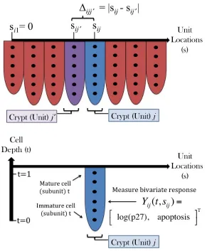
For simplicity of exposition we now describe the modeling framework for bivari-ate functional data. Consider hierarchical data (groups-subjects-units) where within each subject are several units on which two response curves are observed. With-out loss of generality, assume that the units within a subject are aligned on a one-dimensional grid and define the relative spatial location sij ∈ R to be the distance of unit j = 1, . . . , Mi from the first unit within subject i = 1, . . . , N. Let Yij(t,sij) =
[Yij1(t,sij),Yij2(t,sij)]T be the continuous bivariate response measured at subunitt∈ T within unit j at spatial location sij within subject i of group G(i) = 1, . . . , D. Our model is
Yij(t,sij) = µG(i)(t) +Zi(t) +Qi(t,sij) +ij(t) (2.1)
Qi(t,sij) = Wij(t) +Ui(sij) where Wij(t) is a square-integrable, bivariate random process depending only on the subunitt;Ui(sij)is a bivariate random spatial process depending only on the unit spatial location, sij, whose correlation structure models the spatial dependence between units within subjecti. This leads to our parsimonious model:
Yij(t,sij) = µG(i)(t) +Zi(t) +Wij(t) +Ui(sij) +ij(t). (2.2)
We assume that µG(i)(t) are modeled parametrically, and for identifiability we as-sume thatZi(·),Wij(·),Ui(·)andij(·)are mean zero, uncorrelated bivariate random processes.
2.2.1 Model Assumptions
Henceforth, we use superscripts p = 1, 2 to denote the components of bivariate vectors. For example, the superscriptp =1 identifies the first component,Yij1(t,sij), of the bivariate responseYij(t,sij), and p =2 identifies the second componentYij2(t,sij). It is assumed that the functions are observed at a dense, balanced design, that is, tij` = t` for ` =1, . . . , L and that there is an equal number of curves across subjects, that is, Mi ≡M.
In model (2.2), eijp(t) are assumed to be white noise processes with eijp(t) i.∼i.d.
N(0,τp2)ande1ij(t) uncorrelated withe2ij(t). The bivariate random processesZ(t) and
W(t) have covariance operators KZpp0(t,t0) = Cov{Z
p i(t),Z
p0 i (t
0)} and KW
pp0(t,t0) = Cov{Wijp(t),Wijp0(t0)}, respectively, for p,p0 = 1, 2 leading to the 2×2 covariance matrices KZ(t,t0) = {KZpp0(t,t0)}p,p0∈{1,2} and KW(t,t0) = {KWpp0(t,t0)}p,p0∈{1,2}. The specific form of these covariance matrices is presented in Section 2.2.3.
For modeling the spatial dependence between units, we assume that Ui(·) = [Ui1(·),Ui2(·)]T is a mean-zero and second-order stationary, isotropic random bivari-ate process that is measured at locations si1, . . . ,siM ∈ [0, H] for sij ∈ R. The as-sumption of stationarity is important because it means that the spatial covariance between units within a subject only depend on the distance between the unit loca-tions and not on the unit localoca-tions themselves. Notationally, we represent the spatial covariance function as Cpp0(∆ijj0) = Cov{U
p
i(sij),U p0
the covariance between Ui(sij) and Ui(sij0) is the 2×2 spatial covariance matrix
C(∆ijj0) = {Cpp0(∆ijj0)}p,p0∈{1,2} and its specific form is presented in Section 2.2.2. Moreover, we assume that the spatial covariance approaches zero as the distance between units increases,Cpp0(∆) →0 as∆ → ∞, an assumption essential to the esti-mation procedure in Section 2.3.
2.2.2 Bivariate Matérn structure for spatial covariance
Due to its flexibility, we consider the Matérn class to model the spatial covariance. Specifically, assume that the covariance matrixC(·) has a bivariate Matérn structure. IfCpp0(∆)is the spatial cross covariance function forUp(s1)andUp
0
(s2)that are
mea-sured at locationss1,s2 ∈ D ⊂Rwhere∆=s1−s2, then for p,p0 =1, 2, the bivariate
Matérn class of cross covariance functions definesCpp0(∆) = σpp0M(∆|νpp0,app0) with Matérn correlation function M(∆|ν,a) = {21−ν/Γ(ν)}(a|∆|)νKν(a|∆|), where Kν is
a modified Bessel function of the second kind and ν > 0 and a > 0 are
smooth-ness and scale parameters, respectively (Apanasovich et al. 2012; Gneiting et al. 2010; Matérn 1986). (For extension to d-dimensional locations, one only needs to replace the absolute value in the correlation function with the Euclidean norm.)
The smoothness parameter ν of the Matérn correlation function governs the
dif-ferentiability of the process, where larger values of ν indicate a smoother process.
(Special cases of the Matérn correlation function include the exponential (ν = 1/2)
and Whittle (ν = 1) models, as well as the Gaussian when ν = ∞.) With ν fixed, a
governs how fast the correlation decays with distance. Larger values of a indicate a faster decay, and 1/a is sometimes called the correlation length. The auto-covariance componentsC11(∆)andC22(∆)are common Matérn covariance functions. For
exam-ple σ11 represents the spatial variance of the process and is known as the partial sill
in the spatial literature. The spatial cross covariance, represented by σ12, is a
func-tion of the cross-correlafunc-tion parameterρ12 and each of the marginal spatial variances:
σ12 =σ21 =ρ12 √
σ11σ22.
2.2.3 Modeling of functional processes
In keeping with the multilevel terminology used in Di et al. (2009) and Staicu et al. (2010), we call Zi(t) level 1 functions and Wij(t) level 2 functions. Let Zi(t) and Wij(t) be processes in L2[0, 1]× L2[0, 1], and let {
k ≥ 1} and {φφφW` (t) = [φW`1(t),φW`2(t)]T : ` ≥ 1} be two sets of orthogonal
bi-variate basis functions in L2[0, 1]× L2[0, 1] with respect to the norm induced by
the inner product < (f1,g1),(f2,g2) >=
R
f1f2+
R
g1g2. The functional processes
can be expanded as Zi(t) = ∑∞k=1ξi,kφφφZk(t) and Wij(t) = ∑∞`=1ζij,`φφφW` (t) where
ξi,k and ζij,` are random basis coefficients calculated as < Zi(t),φφφZk(t) > and
< Wij(t),φφφW` (t) >, respectively. Using this expansion, we can rewrite model (2.2):
Yij(t,sij) = µG(i)(t) +∑∞k=1ξi,kφφφkZ(t) +∑∞`=1ζij,`φφφW` (t) +Ui(sij) +ijt. In practice, fi-nite truncations are used instead; let NZ and NW be the truncation values for Zi(·) and Wij(·), respectively, leading to the simplified model
Yij(t,sij) =µG(i)(t) +
NZ
∑
k=1
ξi,kφφφZk(t) +
NW
∑
`=1
ζij,`φφφW` (t) +Ui(sij) +ijt. (2.3)
There are several ways to chose the basis functions by either using predetermined bases such as Fourier or wavelets or using the basis formed by the eigenfunctions of the covariance operator. We opt for the latter choice; if KZ and KW are the co-variance operators of Z and W respectively, then by applying Mercer’s Theorem (Indritz 1963) to multivariate data the eigenfunctions are obtained from the spec-tral decompositions of the respective covariance functions. In particular, KZ(t,t0) = ∑∞k=1λZkφφφkZ(t){φφφkZ(t
0)}T and KW(t,t0) = ∑∞
`=1λW` φφφW` (t){φφφW` (t
0)}T. In this case, the
function expansions leading to (2.3) are known as Karhunen-Loève expansions (Karhunen 1947; Loève 1945) and the random coefficients ξik and ζij,` as functional principal components (FPC) scores. Furthermore the FPC scores ξik and ζij,` are as-sumed to be uncorrelated overkand`respectively, are zero-mean, and have variances
λkZ and λW` , respectively. Additionally, following the assumption thatZi and Wij are uncorrelated, it is assumed that {ξi,k : k = 1, 2, . . .} are uncorrelated with{ζij,` : ` = 1, 2, . . .}.
2.2.4 Notation for balanced design
To facilitate exposition of the estimation section, we rewrite in matrix form the co-variance operators in Section 2.2.1 for a dense, balanced design. Let t = [t1, . . . ,tL]T
vec-tor Wij = [Wij1,T(t),Wij2,T(t)]T has covariance matrix Var(Wij) = KW defined analo-gously.
For the spatial process, let si = [si1,si2, . . . ,siM]T be the M×1 vector of unit
lo-cations for subject i with the convention that si1 = 0, where sij is the relative dis-tance of unit j from the first unit location. The M×M matrix ∆i = {∆ijj0}Mj,j0=1 is that which is formed from every pairwise distance between the M units located in subject i = 1, . . . , N. The (matrix-valued) block covariance matrix of Ui(si) = [Ui1,T(si),Ui2,T(si)]T is C(∆i) which has blocks Cpp0(∆i). Furthermore, assuming the bivariate Matérn covariance structure in Section (2.2.2) gives the parametric form Cpp0(∆i) =σpp0M(∆i|νpp0,app0).
2.3
Estimation
To address our primary objectives of estimating the group means and understand-ing how the distance between units affects the spatial correlation, we have developed an estimation procedure that identifies the key components that account for variation at each hierarchy level. Estimates of the Matérn parameters will identify the spatial signal across units as well as the strength and direction of the spatial correlation be-tween the two response curves that we model jointly. Moreover, once estimates of the covariancesKW, KZ, Ci and the error variancesτ12and τ22 are obtained, one can
es-timate the group mean functions µG(i)(t) using generalized least squares regression with estimated covariance. The outline of our estimation procedure is:
1. Estimate the bivariate Matérn parameters for the spatial covariance (Section 2.3.1);
2. EstimateKZ and KW using method of moments (Section 2.3.2);
3. Obtain eigenfunctions and eigenvalues for KZ and KW through MFPCA and also estimate the error varianceτp2 for p =1, 2 (Section 2.3.3);
2.3.1 Spatial covariance estimation
Estimation of the spatial covariance matrix is done in two parts: 1) we define a raw estimator based on method of moments and 2) fit a parametric bivariate co-variance structure that leads to a positive semi-definite, smoothed coco-variance estima-tor. Essential to part one is the assumption that the spatial correlation approaches zero as the distance between observations increases. Although the correlation will never be exactly zero, using this we can assume that there exists some correlation range ∆∗ (chosen based on scientific or expert knowledge) for which units can be considered uncorrelated if the distance between them exceeds the correlation range: Cpp0(∆)≈0 if ∆ ≥∆∗.
The preferred moment-based estimation method in the spatial literature is based on the (cross) semivariogram (Cressie 1993), defined as half of the variance of the difference in residuals for observations separated by a given distance. Our setting re-quires a generalization of this standard approach because spatial variation is just one piece of the complex model given in (2.2). For spatial lag δ <∆∗, denote byN(δ,e)
the set (across all subjects and all groups) of unit-pairs within the same subject whose distance from one another is within a tolerance, e, of δ. We select e so that at least
30 distinct unit-pairs are in N(δ,e) (see Journel and Huijbregts 1978; Cressie 1993,
Ch. 2). Define N(δ,e) to be the same for all spatial lags δ > ∆∗. In summary, for
∆ijj0 =|sij−sij0|,
N(δ,e) =
(i,j,j0) : j6=j0 & ∆ijj0 ∈ [δ−e,δ+e] if 0<δ <∆∗
{(i,j,j0) : j6= j0 & ∆ijj0 ≥∆∗} ifδ ≥∆∗.
(2.4)
Define Gijjpp00(t,t0) = 12{Y
p
ij(t,sij)−Y p0 ij0(t
0,s
ij0)}2 − 12{Y
p
ij(t,sij) −Y p0
ij (t0,sij)}2, on which the following method of moments estimators are based.Gijjpp00(t,t0) is only use-ful for observations from two different units since Gijjpp00(t,t0) = 0 if j = j0, and it is not unbiased for the (cross) semi-variogramγpp0(∆ijj0) =CU
the (cross) semivariogram for spatial lag δ>0 as
e
γpp0(δ,e) = 1
L2|N(δ,e)|
∑
(i,j,j0)∈N(δ,e)
∑
t,t0Gijjpp00(t,t0), (2.5)
where| · | indicates cardinality of a set. Forδ =0, define
e γ0pp0,
e =
1
L|N(∆∗,e)|(i,j,j0)∈N
∑
(∆∗,e)t∑
=t0Gijjpp00(t,t0). (2.6)
Let ¯ηa,pp0 = L−1∑t=t0ηpp0(t,t0) and ¯ηb,pp0 = L−2∑t,t0ηpp0(t,t0). Then (2.5) has ex-pectation E{γepp0(δ)} =Cpp0(0)−Cpp0(δ) +η¯b,pp0, and (2.6) has expectation E{
e γ0pp0} =
Cpp0(0)−Cpp0(∆∗) +η¯a,pp0 which simplifies to E{γe
0
pp0} ≈ Cpp0(0) +η¯a,pp0 by the as-sumption thatCpp0(∆) ≈0 if ∆≥∆∗. Hereηpp0(t,t0) differs from the nugget effect in that it also includes the level 2 functional covariance operator. Our estimation pro-cedure will account for the nuisance parameters ηpp0(t,t0), but only the parameters of the bivariate Matérn covariance are of interest. Then raw estimator for the (cross) covariogram becomes
e
Cpp0(δ) =
e
γ0pp0 if δ=0;
e
γpp0(∆∗)−γepp0(δ) if 0 <δ<∆
∗
;
(2.7)
we set Cepp0(δ) = 0 if δ ≥ ∆∗. When 0 < δ < ∆∗, the covariance estimator given in
(2.7) is unbiased. For δ = 0, Cepp(0) = γe0pp0 is upwardly biased due to the positive term ¯ηa,pp0.
The moments-based raw estimate of the spatial covariance from (2.7) is neither guaranteed to be smooth nor positive semi-definite. To obtain a smoothed esti-mate, (2.7) provides the foundation for estimating the Matérn parameters through a procedure that emulates maximum likelihood but uses the estimated covariance in place of data. In order to find a suitable function f to maximize, assume there exists some unobserved, bivariate Gaussian spatial process Q(s) measured at lo-cations si = [si1, . . . ,sim]T, sij ∈ R, for j = 1, . . . , m within subject i = 1, . . . , n. The pairwise distances ∆ijj0 = |sij−sjj0| form the distance matrix ∆i = {∆ijj0}m
j,j0=1.
Let Σ(∆i;θ,η) be a parametric covariance matrix with elements Σpp0(∆ijj0;θ,η) =
pa-rameters we wish to estimate, and η indicates the nuisance parameters. Now, let
Qi indep∼ N2m 0,Σ(∆i;θ,η)
where Qi = [Q1,T(si),Q2,T(si)]T. Furthermore, assume that all subjectsi are observed on the same equally spaced m×1 grid of pointssgrid
with the convention sgrid,1 =0, and sgrid,m <∆∗, so that ∆i ≡ ∆grid for all i, and the
largest pairwise distance between locations will be less than∆∗. Thus, theQiare i.i.d. multivariate normal random variables with covariance matrixΣ(∆grid;θ,η).
The log-likelihood function, minus arbitrary constants, is `(θ,η;q1, . . . ,qn) =
−1/2∑in=1
h
log|Σ(∆grid;θ,η)|+nqiTΣ−1(∆grid;θ,η)qioi, which can alternatively be written in terms of the sample covariance Cq = 1/n∑in=1qiqTi by using the trace:
`(θ,η;q1, . . . ,qn) = −n/2hlog|Σ(∆grid;θ,η)|+TrnΣ−1(∆grid;θ,η)Cqoi. Since we do not observe the data q and, hence, cannot directly use the sample covari-ance Cq in the likelihood, we must use a covariance estimate based on (2.7) as a substitute. Evaluating (2.7) for each element in ∆grid gives the estimated
co-variance matrix Cegrid = {Cepp0(∆grid)}p,p0∈{1,2}, which we use in place of Cq.
Note that E(Cegrid) = {σpp0M(∆grid|νpp0,app0) + η¯a,pp0I}p,p0∈{1,2}, where I is the
m×m identity matrix. Lastly, we maximize the function f(θ,η;y1, . . . ,yn) =
−n/2hlog|Σ(∆grid;θ,η)|+TrnΣ−1(∆grid;θ,η)Cegrid oi
to find the bivariate Matérn
parameter estimatesθb, resulting in the smooth estimatorCb =C(θb).
To ensure the estimated parameters produce a valid bivariate Matérn structure in which the marginal covariances Cb11 and Cb22 and the entire bivariate covariance
ma-trix Cb are positive semi-definite, we implement the three-step maximum likelihood
algorithm proposed by Apanasovich et al. (2012):
1: Fit the marginal models to get the parameters σpp, νpp and appfor p=1, 2. 2: Defineν12 = (ν11+ν22)/2+∆Afor∆A≥0, a12 = (a211+a222)/2+∆B for∆B ≥0
and σ122 =ρ212(σ11σ22)∏3k=1ψ
(k)
12 .
3: Holding the univariate parameters σpp, νpp and app fixed from Step 1, fit the bivariate model and estimate ∆A, ∆B, and ρ12.
The ψ(ppk)0 in Step 2 are defined for components p,p0 as ψ
(1)
pp0 =
B(νpp0,d/2)2/B{(νpp + νp0p0)/2,d/2}2, ψ
(2)
pp0 = (appap0p0/a2pp0)2∆A, and ψ(pp3)0 = Γ2{(νpp + νp0p0)/2}a
2νpp
pp a
2νp0p0
p0p0 /{a
2(νpp+νp0p0)
are possible by slight modifications of this algorithm; see Apanasovich et al. (2012). Initial values of the Matérn parameters for the maximum likelihood procedure can be found through weighted least squares as shown in Appendix A.3.
2.3.2 Raw functional covariance estimates
In order to implement FPCA, we will need to find asymptotically consistent es-timates of KZ(t,t0) and KW(t,t0). We do this in a manner similar to that in Staicu et al. (2010) and Di et al. (2009), utilizing the same notions of total and between co-variance that are analogous to the co-variance decomposition found in mixed ANOVA models. Define the total covariance of unit-level functions measured within the same unit j as KTotal,Y pp0(t,t0) = Cov{Y
p
ij(t,sij),Y p0
ij (t0,sij)} and the between covariance of the unit-level functions that are distance ∆ijj0 > 0 apart as KBetween,Y pp0(t,t0,∆ijj0) = Cov{Yijp(t,sij),Y
p0 ij0(t
0,s
ij0)}. In terms of model (2.2), the total and between covari-ance quantities can be written KTotal,Y pp0(t,t0) = KZpp0(t,t0) +KWpp0(t,t0) +Cpp0(∆ = 0) +τp2I(t = t0,p = p0) and KBetween,Y pp0(t,t0,∆ijj0) = KZpp0(t,t0) +Cpp0(∆ijj0). These covariance quantities and their decompositions in terms of model (2.2) are key in our estimation method, particularly because they provide an intuitive method of moments-based approach with desired consistency properties.
Define the moments-based nearest neighbor estimator
b
KZpp0(t,t0) = 1
|N(∆∗)|(i,j,j0)
∑
∈N(∆∗){Yijp(t,sij)−Y¯Gp(i)(t)}{Yp
0
ij0(t
0
,sij0)−Y¯ p0 G(i)(t
0)}
, (2.8)
where p,p0 = 1, 2, N(∆∗) is given in (2.4) and ¯YGp(i)(t) is the group mean at t over all unit locations and all subjects in the group to which subject i belongs. This estimator makes use of the property that KY
Between,pp0(t,t0,∆∗) ≈KZpp0(t,t0) since
Cpp0(∆)≈0 if ∆ ≥∆∗.
To estimate KW(t,t0) we diverge from the methods of Staicu et al. (2010) and Di et al. (2009). Consider the residuals Rijp(t,sij) = Y
p
ij(t,sij)−bL
p
i(t) for some smooth estimator bL
p
i(t) = µb
p
G(i)(t) +Zb
p
i(t) obtained using penalized regression splines or similar methods to smooth the pooled data across units for each subject i and each bivariate response component p = 1, 2. We can model the residuals as Rij(t,sij) =
Cov{Rijp(t,sij),R p0
ij(t0,sij)}, which has the decomposition KRTotal,pp0(t,t0) = KWpp0(t,t0) +
Cpp0(0) +τp2I(t = t0,p = p0). Let KWpp0,Inflated(t,t0) = KWpp0(t,t0) +τp2I(t = t0,p = p0) denote the covariance process of Wij(t) that is inflated by the error. Its estimator is given by
b
KWpp0,Inflated(t,t0) = 1 NM
N
∑
i=1 M
∑
j=1
{Rpij(t,sij)R p0 ij(t
0
,sij)} −Cbpp0(0), (2.9)
whereCbpp0(0) is defined in (2.7).
2.3.3 Multivariate multilevel FPCA
Multilevel FPCA (MFPCA) as presented in Di et al. (2009) retrieves the eigenval-ues and eigenfunctions that comprise the covariance expansion for level 1 and level 2 univariate functional processes observed with error by implementing FPCA on smoothed covariance matrix estimates. We introduce a novel adaptation of MFPCA that incorporates the multivariate structure for multilevel spatial functional data.
Since we are assuming the curves are observed with error, we must smooth the raw level 1 and level 2 covariance estimates given in (2.8) and (2.9) in order to imple-ment MFPCA. For level 1, we use (2.8) to form the raw matricesKcppZ0 for p,p0 = 1, 2 and smooth each univariate and cross covariance separately to obtainKfsm,Z pp0. These individually smoothed matrices combine to form the bivariate smoothed covariance
f
KsmZ . The intuition behind smoothing the submatrices separately and then combining them into the bivariate matrix versus combining the raw estimates first and smooth-ing the bivariate matrix is that the delineations between the submatrices need not be smooth within the bivariate matrix.
For level 2, we use (2.9) to form Kcinflated,W pp0 for p,p0 =1, 2. Since the diagonals of the univariate matrices Kcinflated,11W and Kcinflated,22W are inflated by the error variances
τ12 and τ22, respectively, we ignore the diagonals when smoothing. After smoothing
c
Kinflated,W pp0 separately for p,p0 =1, 2 to obtainKfsm,W pp0, the smoothed estimates
com-bine to form the bivariate covariance matrix KfsmW. In contrast to the raw covariance
estimate KcinflatedW , the smoothed level 2 bivariate matrixKfsmW is no longer inflated by
variances,
b τp2 =
1 L
L
∑
t=1
n b
KppW,Inflated(t,t)−KeWpp,sm(t,t) o
. (2.10)
In implementing MFPCA, we find the eigenfunctions e(t) and the eigenvalues
b
λ of the smoothed bivariate covariance estimates Kfsm for both level 1 and level
2 processes. The truncated spectral decompositions of these covariances as pre-sented in Section 2.2.3 lead to the estimators KcZ(t,t0) = ∑
NZ
k=1bλZkekZ(t){ekZ(t0)}T and c
KW(t,t0) = ∑NW
`=1bλW` eW` (t){eW` (t0)}T of the cross covariance matrices for the level 1
and 2 processes. The truncation values NZ and NW are chosen based on the propor-tion of variapropor-tion explained by the eigenvalues as suggested in Di et al. (2009). Using level 1 as an example, specify a cumulative explained variance threshold P1 and and
individual explained variance threshold P2. Define NZ =min{k: p1Zk ≥P1,pZ2k <P2}
where pkZ1 = ∑ki=1bλZi /∑nj=1bλZj, pZk2 = bλZk/∑nj=1bλZj and the positive eigenvalues are
the first n≥k eigenvalues. NW for level 2 is found analogously.
2.3.4 Estimate group mean functions
Assume that the group means are modeled parametrically as µG(i)(t) = Xiβ. Once the covariance estimates have been found, we can use generalized least squares (GLS) regression assuming known (or estimated) covariance to estimate the diet means. Let Yp,ij = [Yijp(t1,sij), . . . ,Yijp(tL,sij)]T be the L×1 vector obtained by stack-ing the responses over subunits tk, k = 1, . . . , L, for component p in unit j within subject i. Stacking Yp,ij over units j = 1, . . . , M yields the ML×1 vector Yp,i, which is then stacked over p to form the 2ML×1 overall response vector for subject i,
Yi = [Y1,Ti,Y2,Ti]T. Define Vi,pp0 = Cov(Yp,i,Yp0,i). Then the response vector Yi for subject i = 1, . . . , N has the cross covariance matrix Vi = {Vi,pp0}p,p0∈{1,2}. Combin-ing the estimates from previous sections gives Vbi,pp0 = JM⊗KcppZ0 +IM⊗KcWpp0 +
b
CppU0(∆i)⊗JL+bτp2δpp0IML, where ⊗ indicates the Kronecker product, JM is a M×M matrix of ones, JL is a L×L matrix of ones, IM is the M×M identity matrix, IML is
the ML×ML identity matrix, and δpp0 = 1 if p = p0, 0 else. Employing GLS estima-tion with the estimated cross covariance matrix, we obtainµbG(i)(t) =XiβbGLSwhere b
2.4
Simulations
The purpose of our simulations is two-fold: 1) compare our model with simpli-fied versions to assess performance gain (Scenarios 1-4), and 2) explore robustness to model misspecification (Scenarios 5 & 6). For Scenarios 1-4 we consider four estimat-ing models:
1. Full (FULL): the multivariate spatial model in (2.3);
2. Non-spatial (NS): the model from (2.3) with no spatial process (Ui(s)≡0); 3. Univariate (UNIV): the model from (2.3) applied separately to each response;
4. True-GLS (TRUE): results of GLS estimation when using each subject’s true cross covariance matrixVi(Section 2.3.4) that comes from the correct generating model.
The next sections discuss the simulation specifications and results for Scenarios 1-4 and briefly summarize our findings for Scenarios 5 and 6. The latter scenarios are discussed in more detail in Appendix A.2.
2.4.1 Data generation
In Scenarios 1-4 we generate data from FULL according to the differing sample sizes and spatial cross-correlations shown in Table 2.1. All scenarios use 100 Monte Carlo (MC) replications. There are D=2 groups with mean functions µ1d(t) = 3t+d
and µ2d(t) = d−t+t2 for d = 1, 2. Each group has N = 10, 50 subjects, M = 20
units per subject, and L=30 subunits per unit that are equally spaced in [0, 1]. Unit locations {sij : j = 1, . . . , M} for subject i are assumed i.i.d. and are obtained by generating from the uniform distribution on [0, 15] to emulate the colon slices in the colon carcinogenesis data which can be up to 15 millimeters in length.
Table 2.1: Specifications for Scenarios 1-4
ρ12 =0.8 ρ12 =0.2
The bivariate Matérn parameters are ρ12 = 0.2, 0.8, σ11,σ22 = 1, ν11,ν22,ν12 = 1,
and a11,a22,a12 = 4, chosen so the auto- and cross-correlations decay to zero at
distances of approximately 1 unit. For the level 1 process Zi(t) = ∑NZ
k=1ξi,kφφφ
Z k(t), NZ = 2 with orthogonal eigenfunctionsφφφZ1(t) = [sin(2πt),
√
3/2(2t−1)]T, φφφ2Z(t) = [cos(2πt),
√
5/2(6t2−6t+1)]T and eigenvalues λZ1 = 1.25, λZ2 = 0.25. For the
level 2 process Wij(t) = ∑NW
`=1ζij,`φφφW` (t), NW = 2 with orthogonal eigenfunc-tions φφφW1 (t) = [sin(4πt), cos(6πt)]T, φφφW2 (t) = [cos(4πt), sin(8πt)]T and
eigenval-ues λW1 = 1.25, λW2 = 0.375. FPC scores are generated as ξi ∼ N 0, diag(λZ1,λ2Z)
and ζij ∼ N 0, diag(λW1 ,λW2 ). Finally, the error is generated from eij = [e1ij,e2ij]T ∼ N(0, diag(τ12,τ22)) whereτ12,τ22 =0.075.
2.4.2 Computational Details
We compare the performance of correctly specifying FULL to the performance of NS and UNIV, using TRUE as a baseline. There are several tuning parameters in the estimation method that must be specified. First, ∆∗ (Section 2.3.1) is set to be 2.5, which is conservative based on the spatial correlation decay to zero around 1. Furthermore, the tolerancee is set such that each spatial lag has around 100 triplets
entering its nearest neighbor set, corresponding to e =0.1 for N = 10 and e = 0.02
for N = 50. We found that an equally spaced grid sgrid of m = 50 points (Section 2.3.1) works well for spatial estimation for this simulation. In practice, m is a tuning parameter that should be chosen to be large enough to capture the features of the covariance matrix but small enough so that the dimensionality of the covariance matrix remains reasonable and computationally feasible. Estimate NZ and NW using the cumulative explained variance threshold P1 = 0.95 and an individual explained
variance threshold P2 =1 (see Section 2.3.3).
Prior to implementing the bivariate estimation methods, we recommend scal-ing each univariate response so that the variances are on a similar scale, particu-larly since scalar variances for the scores from MFPCA are estimated from infor-mation from both responses. For example, one can use Yijp(t,sij)/sp where sp =
[(NML)−1∑i,j,t{Yijp(t,sij)−Y¯p}2]1/2 for L subunits, M units and N subjects, and ¯Yp is the overall mean for response p. Also, we place constraints on the smoothness pa-rametersνpp0 ∈ (0.1, 5) and the range parameters 1/app0 ∈ (min
i,j,j0{δijj
0}, max
i,j,j0 {δijj
0}) so