ABSTRACT
ZAMANI FARAHANI, VAHRAZ. State Estimation for Volt/VAR Control on Active Power Distribution Systems. (Under the direction of Dr. Mesut E. Baran).
The Meter Placement problem on the distribution feeders is addressed in Chapter 5. First, available literature regarding this problem is reviewed, after which the problem is formulated for VVC application, especially CVR application. The heuristic approaches have been proposed, based on the extensive studies and sensitivity analyses, to obtain guidelines for placing the different types of measurements on the system. The proposed schemes have two stages. First stage starts by placing the meters by the rules. At the second stage, an efficient search scheme has been implemented to find the minimal set of measurement for VVC. These schemes are flexible in that it allows incorporation of different metering options and robustness measures. Finally, the performances of these methods are assessed on the IEEE prototype test feeder.
State Estimation for Volt/VAR Control on Active Power Distribution Systems
by
Vahraz Zamani Farahani
A dissertation submitted to the Graduate Faculty of North Carolina State University
in partial fulfillment of the requirements for the degree of
Doctor of Philosophy Electrical Engineering
Raleigh, North Carolina 2014
APPROVED BY:
_______________________________ ______________________________ Dr. Mesut E. Baran Dr. Subhashish Bhattacharya
Committee Chair
_______________________________ ______________________________
Dr. Aranya Chakrabortty Dr. Sujit Ghosh
_______________________________ ________________________________
DEDICATION TO MY PARENTS
BIOGRAPHY
ACKNOWLEDGMENTS
First and foremost, I would like to express my sincere appreciation to my advisor, Professor Mesut E. Baran, for his persistent guidance as well as teaching how to conduct the practical research. Prof. Baran’s deep knowledge in power systems and his unique approach to solve the problems have been very inspirational to my research and development at NC State. I hope to be privileged to benefit from his mentorship and collaboration throughout my future career.
I am grateful to my committee members, Professor Sujit K. Ghosh from Statistics Department, Dr. Subhashish Bhattacharya, and Dr. Aranya Chakrabortty for their valuable suggestions and helps. I would also like to thank Professors Iqbal Husain and Alex Huang, by providing the great research environment at Future Renewable Electric Energy Delivery and Management (FREEDM) Systems Center to conduct my research.
It has been a great pleasure to work with EPS group, Dr. Hossein Hooshyar, Dr. Zhan Shen, Mr. Urvir Singh, Mr. Moyeen Kazi, Mr. Sanujit Sahoo, Mrs. Yue Shi, Mr. Kyle Barth, Mr. Bharadwaj Vasudevan, and Mr. Travis Tippens at the FREEDM Systems Center.
I appreciate the assistance from the staff members of the FREEDM Systems Center and the graduate office of the ECE department, including Dr. Pam Carpenter, Dr. Michael Devetsikiotis, Mr. Rogelio Sullivan, Ms. Karen Autry, Ms. Colleen Reid, Ms. Cailan Mang, and Ms. Elaine Hardin.
I would like to thank my colleagues and friends at NC State University, especially in FREEDM Systems Dr. Babak Parkhideh, Mr. Hesam Mirzaee, Dr. Saman Babaei, Mr. Behzad Nabavi, Dr. I. Safak Bayram, Dr. Habib Rahimi, Mr. Sina Parhizi, Dr. Gangyao Wang, Mr. Daniel Fregosi, Mr. Sumit Dutta, Mr. Arun Kadavelugu, Dr. Edward van Brunt, Mrs. Ghazal Fallahi, Mr. Mohammad Ali Rezaei, Mr. Maziar Vanouni, Mr. Nima Yousefpoor, Mr. Tom Nuddel, Mr. Anken De, and Mr. Mohammad Etemadrezaei.
My deepest appreciation goes toward my parents and family, father and mother: Mr. Mojtaba Zamani Farahani and Mrs. Vila Gharagouzlou, my dear sisters: Mrs. Vishpar Zamani, and Mrs. Roshanak Zamani, who have always encouraged and supported me to pursue my goals.
TABLE OF CONTENTS
LIST OF TABLES ... x
LIST OF FIGURES ... xi
Chapter 1: Introduction ... 1
1-1 Background ... 1
1-2 Dissertation Objective ... 3
1-3 Dissertation Outline ... 4
1-4 Abbreviations... 6
Chapter 2: Real-time Monitoring for Power Distribution Systems ... 9
2-1 Volt/VAR Control on Distribution Systems ... 9
2-1-1 Volt/VAR Control Overview ... 9
2-1-2 Conventional VVC on Distribution Systems ... 10
2-2 DERs on Distribution Systems ... 12
2-2-1 PV Impacts on Distribution Systems ... 13
2-3 SE for Active Power Distribution Systems ... 14
2-3-1 Purpose of State Estimation (SE) ... 14
2-3-2 Challenges of Distribution State Estimation (DSE) ... 18
Chapter 3: State Estimation for Active Power Distribution Systems ... 25
3-1 Overview ... 25
3-2 Distribution System State Estimation Methods ... 25
3-2-1 Probabilistic Approach for Distribution State Estimation [22-24] ... 25
3-2-2 Branch Current Based Three-Phase State Estimation (BCSE) [30, 31, 38, 39] ... 28
3-3 Performance of BCSE Method ... 38
3-3-1 Monte Carlo (MC) Simulation ... 38
3-3-2 Monte Carlo Simulation Sample Size ... 39
3-3-3 Monte Carlo Simulations on BCSE Method ... 42
3-3-4 Bias ... 46
3-3-5 Consistency ... 53
3-3-6 Quality ... 54
3-4-2 Test Results ... 58
3-5 Summary and Conclusion ... 62
Chapter 4: Load Estimation for Distribution Transformers by AMI Data ... 63
4-1 Overview ... 63
4-2 Literature Review ... 64
4-3 What is “AMI”? ... 67
4-4 Actual AMI Data Observation ... 69
4-5 Load Estimation Approach ... 72
4-5-1 Step 1: Load Clustering ... 73
4-5-2 Step 2: Load Estimation Models ... 76
4-6 Test Results... 79
4-6-1 Load Clustering ... 79
4-6-2 Distribution Transformer (DT) Load Estimation ... 83
4-6-3 Performance Test ... 89
4-7 Load Uncertainty Modeling for SE ... 92
4-7-1 Model 1: Proportional Error Approach ... 93
4-7-2 Model 2: Fixed Error Approach ... 96
4-7-3 Model 3: Customer Based Approach ... 98
4-7-4 Comparison of Models ... 99
4-8 Summary and Conclusion ... 101
Chapter 5: Meter Placement on Distribution Feeders for Volt/VAR Control ... 103
5-1 Overview ... 103
5-2 Literature Review ... 104
5-3 Meter Placement Problem ... 107
5-4 Solution Approach ... 109
5-5 Cost of Measurements (CM and VM) ... 111
5-5-1 Metering Accuracy ... 113
5-6 Sensitivity Analyses ... 119
5-6-1 Meter Locations... 119
5-6-2 Impact of Voltage Measurements versus Current Measurements (VM vs CM) ... 128
5-7 Observations ... 131
5-9 The Low Cost Meter Placement Scheme (VM based) ... 138
5-10 The Robust Meter Placement Scheme ... 140
5-11 Test Results and Discussions ... 141
5-11-1 Calculation of Vfor VVC Application ... 142
5-11-2 Results for the Proposed Meter Placement Method ... 142
5-11-3 Results for the Low Cost Meter Placement Method ... 147
5-11-4 Results for the Robust Meter Placement Method ... 148
5-11-5 Comparison of the Proposed Schemes and Discussions ... 150
5-12 Impact of the Load Variations on the Proposed Meter Placement Schemes ... 153
5-13 Impact of the PV Generation on the Proposed Meter Placement Schemes ... 155
5-14 Summary and Conclusions ... 158
Chapter 6: Topology Processing for Distribution Systems by BCSE ... 160
6-1 Overview ... 160
6-2 Robust State Estimation on Power Systems ... 161
6-2-1 What is “Bad Data”? ... 161
6-3 Topology Error Detection and Identification at Transmission Power Systems Level ... 163
At the transmission level of power systems, due to the available redundant measurement, topology error processing is one of the well-defined and well-developed state estimation functions [15]. ... 163
6-3-1 Branch status errors ... 165
6-4 Topology Errors on Distribution Power Systems ... 167
6-4-1 Literature Review ... 171
6-4-2 Topology Error Detection & Identification Using BCSE for Distribution Systems ... 172
6-5 The Proposed Method for Topology Error Identification in Distribution Systems ... 174
6-6 Test Results... 177
6-6-1 Test Results for Case 1 ... 179
6-6-2 Test Results for Case 2 ... 181
6-7 Impact of Topology Changes on BCSE Performance for VVC ... 184
6-8 Summary and Conclusion ... 188
Chapter 7: Conclusion and Future Work ... 190
7-1 Conclusion ... 190
APPENDICES ... 209
APPENDIX 1 – State Estimation Test Results ... 210
APPENDIX 2 - MC Simulations for Std Dev Calculation ... 213
APPENDIX 3 - Voltage Std Dev for Meter Placement ... 216
APPENDIX 4 – Analytical Sensitivity Analysis for a VM and CM Location on a Simplified Feeder ... 217
LIST OF TABLES
Table (1-1): Abbreviations ... 6
Table (2-1): ANSI C84.1Voltage range for 120V [6]. ... 10
Table (4-1): Summary of Performance Metrics for Clustering. ... 81
Table (4-2): ANOVA Table from SAS. ... 84
Table (4-3): ANOVA Table from SAS. ... 86
Table (4-4): Clustering Assignment for Each Individual Load of The DT. ... 88
Table (4-5): Daily RMSE and MAPE for with and without AMI cases. ... 92
Table (5-1): Comparison of Different Approaches for Meter Placement on Distribution Feeders. ... 106
Table (5-2): Cost comparison of voltage and current sensors [102-107]. ... 112
Table (5-3): Steps of meter elimination procedure for IEEE 34 node feeder with 8 measurements. ... 145
Table (5-4): Steps of meter elimination procedure for the robust meter placement scheme. 150 Table (6-1): Output for topology error detection & identification of Case 1. ... 180
Table (6-2): Summary for topology error detection & identification of Case 1. ... 181
Table (6-3): Output for topology error detection & identification of Case 2. ... 182
LIST OF FIGURES
Figure (2-1): Traditional Distribution System [7]. ... 10
Figure (2-2): Voltage profile without Volt-VAR Control under peak load [14]. ... 11
Figure (2-3): Voltage profile after raising the source voltage under peak load [14]. ... 11
Figure (2-4): Voltage profile without Volt-VAR Control under light load after raising setting voltage [14]. ... 12
Figure (2-5): State Estimation framework for Volt/VAR Control ... 15
Figure (2-6): Overview of the active distribution system. ... 17
Figure (3-1): A three-phase line section. ... 31
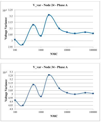
Figure (3-2): Voltage variance for different number of Monte Carlo simulations. ... 41
Figure (3-3): Single-line diagram of IEEE 34 node feeder [87]. ... 43
Figure (3-4): Voltage profile for prototype feeder from PF and BCSE – Case 1 and Phase A. ... 44
Figure (3-5): Branch current magnitude for prototype feeder from PF and BCSE – Case 1 and Phase A. ... 45
Figure (3-6): Estimated system states and true values,x[ , ]Ir Ix , from BCSE and PF; respectively for prototype feeder, real part – Case 1 and Phase A. ... 46
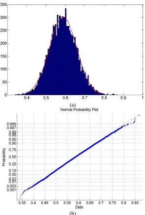
Figure (3-7): Current Magnitude of Branch 1, Phase A; (a) is histogram and (b) is normal probability plot. ... 49
Figure (3-8): Current Magnitude of Branch 1, Phase B; (a) is histogram and (b) is normal probability plot. ... 50
Figure (3-9): Current Magnitude of Branch 32, Phase C; (a) is histogram and (b) is normal probability plot. ... 51
Figure (3-10): Estimated system states and true values,Ix , from BCSE and PF; respectively for phase B – Case 1. ... 52
Figure (3-11): Average of Nfor different MC simulations. ... 54
Figure (3-12): Quality for different measurement error scenarios in Cases 1 and 2. ... 55
Figure (3-13): MC simulation vs Calculation for Ir at Phase A. ... 59
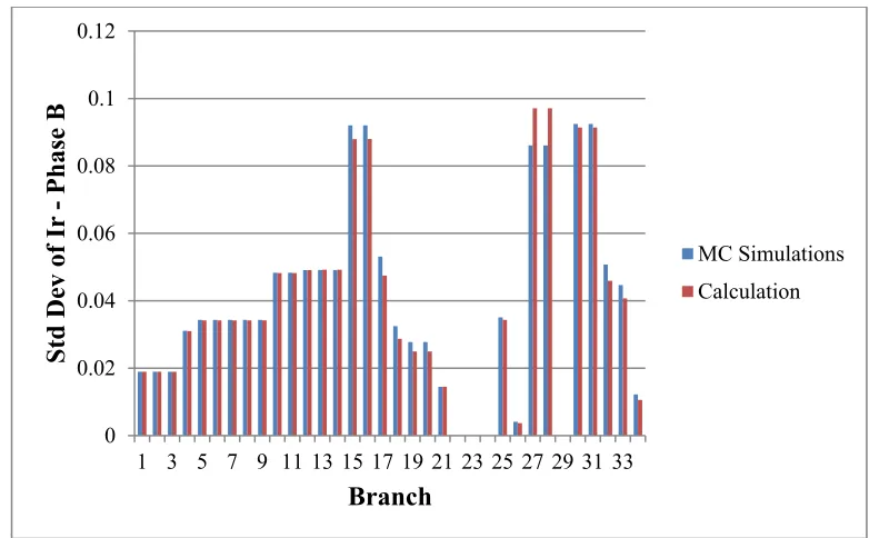
Figure (3-14): MC simulation vs Calculation for Ir at Phase B. ... 60
Figure (3-15): MC simulation vs Calculation for Ir at Phase C. ... 60
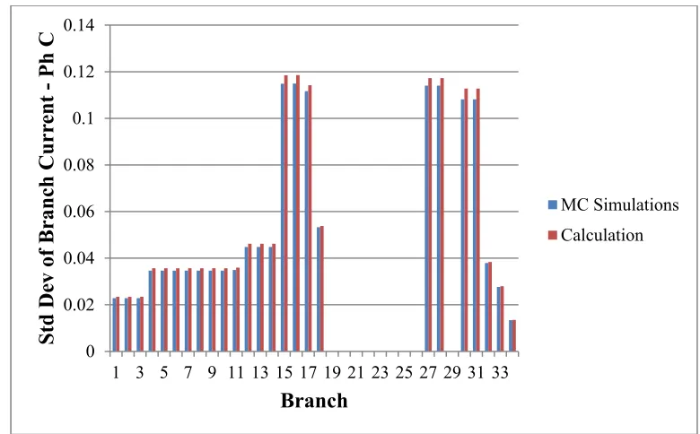
Figure (3-16): MC simulation vs Calculation for standard deviation of branch current at Phase C... 61
Figure (3-17): MC simulation vs Calculation for voltage magnitude at Phase A. ... 61
Figure (4-2): Building blocks of advanced metering from FERC, source: UtiliPoint
International [57, 58]. ... 69 Figure (4-3): One week normalized load profiles for three customers: LD676, LD700, and LD870 [152]... 70 Figure (4-4): Actual load profile for LD676 for one week in spring [152]. ... 71 Figure (4-5): Actual load profile for LD676 for one day in spring. ... 72 Figure (4-6): Distribution transformer load estimation from different load clusters and
Figure (5-6): IEEE 34 node test feeder with M1 at substation and four other VMs (Case 3).
... 117
Figure (5-7): Standard deviation of voltage magnitude with different VM errors (Model 1) for phase B. ... 117
Figure (5-8): Standard deviation of voltage magnitude with different VM errors (Model 2) for phase A. ... 118
Figure (5-9): Moving one CM along the feeder from Cm14 to Cm18. ... 120
Figure (5-10): Standard deviation of voltage magnitude with different CM locations (Model 1) for phase A. ... 120
Figure (5-11): Standard deviation of voltage magnitude with different CM locations (Model 1) for phase B. ... 121
Figure (5-12): Standard deviation of voltage magnitude with different CM locations (Model 2) for phase A. ... 122
Figure (5-14): Boxplots of voltage standard deviation for different locations of one CM. .. 123
Figure (5-15): Moving one VM along the feeder from Vm14 to Vm8. ... 124
Figure (5-16): Standard deviation of voltage magnitude with different VM locations (Model 1) for phase A. ... 125
Figure (5-17): Standard deviation of voltage magnitude with different VM locations (Model 2) for phase A. ... 126
Figure (5-18): Moving one VM along the feeder from the end of the lateral, i.e. Node 33 to the middle of the feeder, i.e. Node 12. ... 127
Figure (5-19): Boxplots of voltage standard deviation for different locations of one VM. .. 128
Figure (5-20): Comparison of maximum and average of voltage standard deviations by adding one new CM or VM. ... 129
Figure (5-21): Comparison of voltage standard deviations for Cases 2 and 3. ... 130
Figure (5-22): Decision graph for three variables [108]. ... 136
Figure (5-23): Algorithm of the mixed meter placement scheme ... 138
Figure (5-24): Algorithm of the low cost meter placement scheme. ... 139
Figure (5-25): Algorithm of the robust meter placement scheme. ... 141
Figure (5-26): Load zones (a) and Initial set of measurements, Zo, four CMs and four VMs (b). ... 143
Figure (5-27): max
σˆV changes by Meter Elimination Procedure. ... 146Figure (5-28): Final measurement set for prototype feeder (2 CMs and 1 VM). ... 147
Figure (5-31): Boxplots of voltage standard deviations for different proposed meter
placement schemes... 151 Figure (5-32): Boxplot of the voltage standard deviation to load variations with the mixed measurement set (3 real-time measurements), blue point: mean. ... 154 Figure (5-33): Boxplot of the voltage standard deviation to load variations with the robust measurement set (6 real-time measurements), blue point: mean. ... 154 Figure (5-34): Average daily load profile and PV generation profile in NC [120, 129]. ... 156 5) Figure (5-35): Boxplot of the voltage standard deviation for different PV generation cases with the mixed measurement set (3 real-time measurements), blue point: mean. ... 157 Figure (6-1): A sample distribution feeder with different faults at primary and secondary side of the network. ... 169 Figure (6-2): Time line for service restoration on distribution systems [1]. ... 170 Figure (6-3): A sample distribution feeder with a fault at Z_SW1 and operated SW1. ... 173 Figure (6-4): The proposed algorithm for topology error detection and identification by BCSE... 176 Figure (6-5): One-line diagram of the IEEE 34 node test feeder for case 1 with three
Chapter 1: Introduction
1-1 Background
To improve efficiency and reliability of the operation of the power distribution systems, implementing an effective real-time monitoring structure is needed to manage and control the distribution systems effectively. Literature survey indicates that utilities have been improving their means of monitoring their distribution systems to advance service reliability as well as energy efficiency thorough their Smart Grid projects [1-6, 10, 12, 131-133]. More recent energy efficiency solutions on the distribution systems are based on the optimization of the voltage profiles to control.
Effective management of distribution systems requires analysis tools that can estimate the state of the system (the operating condition) and predict the response of the system to changing load and weather conditions. The main tool used for system analysis is power flow analysis. But this tool is not very suitable for real-time monitoring as it requires accurate load and system data. Real-time monitoring of the distribution networks has its own challenges, due to radial topology, three-phase unbalanced system, high resistance to reactance ratio, limited real-time measurements, integrating the distributed and renewable energy resources, keep changing topology, and etc. of the distribution systems
others [25-32] are extensions of the conventional state estimation (SE) method for three-phase analysis. SE based solutions are preferred over the power flow approach by considering the uncertainty of the input data and the system, despite of its computational complexity. In this dissertation, the Branch Current based State Estimation (BCSE) method [30] is considered for further studies, it is computationally more efficient and tailored for distribution system characteristics, such as unbalancing in loading and the structure. Furthermore, some statistical techniques are applied for assessing the BCSE performance in this study.
One of the main inputs of SE is the estimated of distribution transformer loads. Previous studies show that the quality of state estimation depends on the load estimation accuracy. Normally, historical data of the customers are used to estimate the loads. By adopting more AMI implementation on the distribution networks, AMI can then provide more up-to-data information about customer loads. To address this challenge, one load estimation method has been implemented to utilize the near real-time data from AMI for enhancing the accuracy of load estimation.
voltage measurements on the feeder by following a set of rules. In the second stage, one efficient sorting procedure is used to select the minimal set of meters. To amend the final set of the measurement, some practical concerns, due to the operation of the distribution systems and measurement loss, are considered.
It is usually assumed that the SE is running in a way that the topology of the system is given without any doubts [17-32]. However, in most of real world conditions, as mentioned before, the state of some switching devices is unknown, for some reasons, or one un-monitored devices, like fuses, are operated. In this case, the current status of the switches plus the given topology are not reliable to run the SE. It is common in the distribution systems that some switches are not monitored by SCADA, and their open/close position in the database of the topology is manually updated by the system operators. The result of these conditions is a topology error in the network. Model topology errors can also occur when the telemetered circuit breaker ON/OFF status is incorrect. Correct network model is crucial to estimate the operating conditions of a system. That is the reason why topology error identification and detection on the distribution feeders by using BCSE method were investigated in this dissertation.
1-2 Dissertation Objective
The main objective of the dissertation at hand is to propose the algorithms for real-time monitoring of distribution systems. The following materials are presented and the main goals of each chapter are explained in the following section.
- Challenges for real-time monitoring of the distribution systems - Assessment of the BCSE method
- Load estimation of distribution transformers by AMI data
1-3 Dissertation Outline
Chapter 2
Basic concepts of the voltage regulation on the distribution system are explained in this chapter. In addition, impacts of distributed energy resources, especially PV solar panels, on the voltage profile of the system are reviewed. As a result, the motivation for adopting SE for monitoring and control of the distribution systems are studied.
Special characteristics of the power distribution systems in comparison to power transmission systems are mentioned and listed, in order to be considered in the implementation of the effective real-time monitoring solutions for distribution systems.
Chapter 3
After presenting the needs for the SE on distribution systems, available methods in literature are considered. Afterwards, the Branch Current based State Estimation method is chosen for further studies. The performance of the BCSE is assessed through statistical measures. Some statistical measures quantified in terms of bias, consistency, and quality are adopted for assessment in this chapter by adopting the statistical tests. For statistical analysis, 10,000 Monte Carlo simulations are performed.
Due to the application of the BCSE for voltage profile estimation, voltage standard deviation calculation has been considered. Here, standard deviation is a measure for quality of the voltage estimation from SE. At the end, the voltage standard deviations from output of BCSE is formulated and calculated. The calculated voltage standard deviations are verified by Monte Carlo simulations.
using the available AMI. This method has two stages. In the initial stage, the given customers are categorized by k-means clustering approach to figure out similar load patterns. First, harmonic-based time series models are developed using historical load data from AMI. When new load data is available from each cluster, the load estimation model can be modified by regression.
This chapter presents a method to improve the historical-based model of load estimation using real time load data from AMI. This method has been tested with actual load data. In addition to present the model for load estimation, impact of the load estimation error on the performance of the BCSE has been investigated too.
Chapter 5
To estimate the voltage profile accurately, more real-time measurements are needed to be placed on the feeder for advanced VVC. This chapter addresses this challenge by proposing solutions based on defining the meter placement problem. Sensitivity analyses are performed for different conditions and situations. Based on these studies, a set of guidelines is developed to determine an initial set of measurements which are reasonably small and are redundant enough to provide the desired level of accuracy. At the second stage, a meter sorting procedure is used to identify the minimal set of meters. Three approaches namely: mixed, low cost, and robust meter placement schemes. The performance of the methods is tested using a prototype distribution feeder.
Chapter 6
problem in the scope of state estimation for real-time monitoring of distribution systems for two common topology changes.
Chapter 7
The overall conclusions of this dissertation at hand are presented in this chapter. In addition, the proposed future work is also outlined within the chapter.
1-4 Abbreviations
In what follows is a list of the abbreviations and their corresponding definitions presented in this dissertation.
Table (1-1): Abbreviations
Abbreviation Definition AMI Automated Metering Infrastructure
ANN Artificial Neural Network
BCSE Branch Current State Estimation
BW Band Width
CAPs Capacitor Bank
CB Circuit Breaker
CES Community Energy Storage
CM Current Measurement
CT Current Transformer
CVR Conservation Voltage Reduction
DER Distributed Energy Resource
Table (1-1): Continued
DMS Distribution Management System
DOE Department of Energy
DR Demand Response
DS Distributed Storage
DSE Distribution State Estimation
DVC Dynamic VAR Compensator
EPRI Electric Power Research Institute
EV Electrical Vehicles
FLISR Fault Location, Isolation, and Service Restoration
GMM Gaussian Mixture Model
IEEE Institute of Electrical and Electronics Engineering
LAV Least Absolute Value
LDC Line Drop Compensation
LF Load Flow
LS Least Squares
LTC Load Tap Changing
MC Monte Carlo
NETL National Energy Technology Laboratory NMC Number of Monte Carlo simulations
NP-hard Non-deterministic Polynomial-time hard
NTP Network Topology Processing
OMS Outage Management System
ONR Optimal Network Reconfiguration
OO Ordinal Optimization
P.U. Per Unit
Table (1-1): Continued
PF Power Flow
PHEV Plug-in Hybrid Electrical Vehicles
PM Power Measurement
PNNL Pacific Northwest National Laboratory
PT Potential Transformer
PV Photovoltaic
RPS Renewable Portfolio Standards
RTU Remote Terminal Unit
SCADA Supervisory Control And Data Acquisition
SE State Estimation
SOC State of the Charge
SST Solid State Transformer
Std Dev Standard Deviation
SVM Support Vector Machine
SW Switch
TP Topology Processor
VM Voltage Measurement
VR Voltage Regulator
VVC Volt/VAR Control
VVO Volt/VAR Optimization
Chapter 2: Real-time Monitoring for Power
Distribution Systems
In this chapter, the necessity of the state estimator for active distribution system monitoring and control is investigated. Utilities are required to provide voltage within a certain band for all of the customers. Hence, Volt/VAR Control (VVC) is one of the smart grid applications will be briefly described. Consequently, VVC challenges for distribution systems with Distributed Energy Resources (DER), especially Photovoltaic (PV) panels, will be reviewed. To understand the current situation of the distribution systems, we need to put all the available measurements and information into the State Estimation (SE) to obtain the system state as the input of the VVC schemes. Implementing SE on distribution systems has its own challenges which will be discussed in both “data” and “system” categorizes below.
2-1 Volt/VAR Control on Distribution Systems
2-1-1 Volt/VAR Control Overview
corrective measures shall be undertaken within a reasonable time to improve voltages to go back to Range A [6].
Table (2-1): ANSI C84.1Voltage range for 120V [6].
Min Max Min Max
Range A (Normal) -5% 5% -8.30% 4.20%
Range B (Emergency) -8.30% 5.80% -11.70% 5.80%
Service Utilization
2-1-2 Conventional VVC on Distribution Systems
In a traditional distribution system, as shown in Figure (2-1), without Volt-VAR control devices, the typical voltage profile under peak load decreases gradually along the feeder. Under heavy load conditions, the node farthest from the substation may have low-voltage violation, Figure (2-2). In order to fix this problem, we need to manually raise the source voltage, Figure (2-3), though this will cause other problems at light load, see Figure (2-4). In other words, Volt-VAR control is needed to deal with all possible normal operation conditions [7].
Figure (2-2): Voltage profile without Volt-VAR Control under peak load [14].
Figure (2-3): Voltage profile after raising the source voltage under peak load [14].
Figure (2-4): Voltage profile without Volt-VAR Control under light load after raising setting voltage [14].
Coordination of CAP and VR: One of the main challenges of local control schemes is the difficulty of coordinating the control between VRs and CAPs. With recent efforts towards extending SCADA at distribution feeder level, it is now becoming possible to coordinate the operation of these devices [8].
2-2 DERs on Distribution Systems
Recently, Renewable Portfolio Standards (RPS) has been proposed in several countries [10]. In America for instance, many states have passed RPS programs with various different targets. California’s target is to reach 33% of total power generation by 2020 and North Carolina’s target is 12.5% by 2021 [10].
system operators need to consider the potential impact of high penetration levels of PVs on traditional distribution power systems and prepare robust measures to mitigate these impacts. Next part, PV impacts on distribution networks has been reviewed.
2-2-1 PV Impacts on Distribution Systems
An increased amount of DERs may have a significant impact on a distribution system [10-14]. The main concerns identified involve reverse power flow, voltage rise, voltage unbalance, voltage fluctuation, improper VR operation, and increased power loss. In what follows, we will give a detailed description of voltage issues from [14]:
Voltage Rise
PV integration can modify feeder voltage profile and raise the voltage close to the location of PVs. When high penetration level of PV is connected in a lightly loaded system, the voltage rise will be significant. If switched capacitor banks are on when the output of PV is maximal or if there are many fixed capacitor banks in the system, this voltage rise will lead to voltage violations on utility planning limits and industry standards. Voltage rise leads to high voltage violation [13].
Voltage Fluctuations
PV is an intermittent resource, therefore its varied output power leads to voltage variations which may cause power quality issues and complaints from customers. The severity of these voltage fluctuations must be assed to ensure that the system will not have voltage violation under any circumstances [14].
Interaction with voltage-controlled capacitor banks, LTCs, and line voltage regulators
the voltage regulators need to move up the tap positions to keep the voltage within limits. The higher the number of operations, the more maintenance required and the shorter the life-cycle of the equipment is. In addition, frequent operations in turn can augment voltage fluctuations and affect power quality. Furthermore, voltage fluctuations may affect the implementation of advanced Volt/VAR Control and Optimization schemes and Conservation Voltage Reduction (CVR) approaches [14].
2-3 SE for Active Power Distribution Systems
2-3-1 Purpose of State Estimation (SE)
Fred Schweppe introduced state estimation to power systems in 1970’s and defined the state estimators as “a data processing algorithm for converting redundant meter readings and other available information into an estimate of the state of an electric power system” [3] for real-time monitoring. A state estimation algorithm which is a result from a combination of two fields, load flow and statistical estimation theory [1], fit measurements made on the system to a mathematical model in order to provide a reliable data base for other monitoring, security assessment and control functions [3, 15]. Inputs of the SE are measurements, system parameters, and structural (topology) information. Then state estimator gives the reliable estimation of the system states, ˆx, to other EMS applications such as contingency analysis, optimal power flow and etc. This process has been shown in Figure (2-5), state estimator is the first block which gathers the all kind of available information about system such as all measurements, parameter values and topology (structural) information and provides the state of the system for other applications.
Figure (2-5): State Estimation framework for Volt/VAR Control
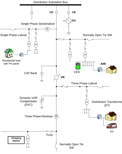
Due to radial topology, three-phase unbalanced system, and high resistance to reactance ration and limited number of real-time measurements, transmission state estimation techniques cannot be applied directly to distribution systems. Therefore, SE in distribution systems is not similar to the one in transmission systems, which is a routine task and a host of established methodologies exist [15]. In addition to smart grid initiatives, some new features, issues, and specifications have been added to the distribution systems by integrating the Distributed Energy Resources (DERs), AMR/AMI, new PE components, etc. These systems are named “Active Distribution Systems” or “Smart Distribution Systems.” A simple overview of an active distribution system is depicted in Figure (2-6).
Traditionally, electric distribution utilities have relied primarily on manual, paper driven process for electric distribution operations. Managing the electric distribution system was handled in mostly a manual fashion with voice communications between responsible parties supported by a collection of independent (stand-alone) computer systems, communication facilities, and device controllers. Distribution Management System (DMS) is a concept that integrates these mostly independent facilities so that the distribution system can be operated in a well-coordinated, highly efficient manner. “A DMS is defined by EPRI as a decision support system to assist the control room and field operating personnel with the monitoring and control of the electric distribution system [1]”. The main part of this energy management system is state estimation and load estimation at the customer, feeder, and substation levels.
Charging Station
AC S
CB
R
VR
CAP Bank
Dynamic VAR Compensator
(DVC)
AMI
Normally Open Tie SW
Normally Open Tie SW CB
DG Single Phase Sectionalizer
Fuse Three Phase Recloser
Residential load with PV panel
Three Phase Lateral Single Phase Lateral
CES Distribution Substation Bus
Distribution Transformer (DT)
EV
Moreover, according to [4], the EDF1 (Electricity of France) R&D developed and implemented a DMS package offering these three functions: Event Synthesis Function (ESF), Fault Location Function (FLF), and Network Restoration Function (NRF). By January 2011, 90% of EDF control centers for distribution network in France have these functions established and nowadays EDF R&D is implementing other three advanced distribution automation functions, which are:
- Distribution State Estimation (DSE). - Volt/VAR Control, and
- Steady-state network reconfiguration.
To provide the optimized voltage profile along the feeders of distribution systems, SE is needed to make the system state available to VVC schemes.
These new infrastructures, components, and devices add more challenges to develop the SE for active distribution networks. These challenges are listed in following part.
2-3-2 Challenges of Distribution State Estimation (DSE)
The main challenges involving these specifications, features, and issues can be categorized as follows:
a- System
In addition, feeder line sections are usually short, un-transposed and have high r/x ratio [25]. These features and specifications are listed below:
Keep changing topology [16, 17, 21, 24, 54, 56, 60, 62, 65-68]:
Since distribution systems involve many protective devices (reclosers, sectionalizers, fuses, etc.) and switches which are normally open during the normal operation and become close when the topology of the serving load changes due to faults or other reasons, therefore keeping the system topology up-to-date has been a major challenge [16]. Some protective devices, such as fuses, are not monitored, but some of them can be monitored. Thus consideration of the effect of these situations is inevitable. Most of the proposed solutions for SE in distribution system considered that the topology is a given accurate and fixed amount [18-47]. A few papers tried to address this challenge in distribution networks, for instance M. Baran et al. [54] presented the algorithm for topology error identification by using the branch current state estimation. R. Singh et al. [66] proposed a recursive Bayesian approach for identification of the network configuration changes in distribution networks. Moreover, Y. Sharon et al. presented a statistical method to detect the changes in the status of switching devices [64]. Therefore, this challenge must be addressed in future solutions for distribution system monitoring and control, by utilizing the outage signal which is available from AMR/AMI and developing the tailored solutions for topology error detection and identification procedures for distribution systems, in both priori and posteriori analyses for topology analysis.
DERs is that they are ‘dispatchable’ and predictable. Different type of DGs are shown in Figure (2-6).
Presence of ‘non-dispatchable’ DG units, e.g. photovoltaic and wind units [72-73]
These DERs are mostly installed at the customer side, like PV panels at the roof of the houses. The type of these power generations is intermittent, non-dispatchable, and heavily depends on weather conditions, such as sunny, windy and other weather conditions. DERs will change the typical load profiles of the customers. Therefore, these new types of generation must be predicted at the accepted level to have a reasonable picture of the distribution system. Different types of DERs are shown in Figure (2-6).
Integration of Electrical Vehicles (EV) and Plug-in Hybrid Electrical Vehicles (PHEV) to the power grid [72-75]
These new types of electrical loads will add new kind of uncertainty to the distribution system which must be considered in the operation of the system, which is shown in Figure (2-6). They can be charged in houses or in charging stations. Because of their size as well as their number, the typical load profile of the feeder has to be changed. Therefore, we need to have an acceptable estimation of their loads on the network and their effects on the system.
Integration of dynamic and static compensator to the power systems at distribution level, such as Dynamic VAR Compensator (DVC), Solid State Transformer (SST), etc. [14, 72, 76, 79, 115]
can provide data of the system such as bounded voltage at the connected node [79]. One DVC is shown in Figure (2-6).
Three-phase unbalances in loading and structure [16, 29, 20, 25-32, 39-40, 43-44, 53-56]
This feature of distribution systems has led to developing the three-phase state estimation to consider all details of the system. It was found that a common single phase SE for transmission systems cannot be used for distribution networks.
Radial and weekly meshed topology [16, 17, 19, 20, 22, 25-32, 39-40, 43-44, 53-56]
This characteristic of the distribution network can help to find the system state with simpler methods in comparison to common approaches for transmission power systems which mostly have a meshed structure.
High r/x ratios [16, 19, 25-32, 39-40, 53-56]
“Fast decoupled state estimation has found wide acceptance in industry and various versions have been implemented in control centers all over the world [15]”. As observed in power flow problem, sensitivity of real (reactive) power equations to changes in the magnitude (phase angle) of bus voltages is very low, especially for high voltage transmission systems with low r/x ratio. On the other hand, these assumptions cannot be applied for distribution systems which have short lines with high r/x ratio [26]. Hence, a full coupled solution must be applied for distribution system SE and it should not be sensitive to this ratio.
b- Data
a) Voltage measurements at substation transformer or voltage regulator [16, 17, 25, 39];
b) Power measurements at substation [16, 17, 25, 39]; and
c) Limited current measurements along the main feeder or laterals [17, 19, 39, 40].
The first question typically asked at this point is: “How many measurements do real distribution systems have?” The answer is: “Many in absolute numbers, but a few percentage-wise.” The average size of the distribution utility we usually work with is about 100-300 subsystems. One subsystem includes from a few hundred branches up to five or six thousand (distribution transformers directly supplying loads are not included in this count). Approximately 2.5% to 5% of branches have either power or current measurements. All LTC transformers and voltage regulators, whose number in a subsystem can reach 50-60, have voltage measurements. At any given time, at least a few subsystems are connected in parallel, creating a large subsystem of up to ten thousand branches [17].
Therefore, we can list the issues, features, and characteristics of the available data in distribution system for SE as follows.
1. Very few measurements are available, sometimes only the voltage and current at the substation, i.e. low redundancy in real-time measurements, e.g. around “0.2-0.3 [20]” [16-23, 37-46, 62-63, 64-69]
This limitation makes the state estimation of the distribution system impossible by just using the real-time data. The usual remedy for this issue is the introduction of pseudo measurement. The main source for these measurements is the estimated loads from historical data such as monthly billing data, yearly random sample, or other ways. Nowadays, by installing the AMR/AMI systems, these load estimation can be more accurate and less delayed from the real-time application.
Load estimation is obtained from historical data and not from real-time measurements; hence the accuracy of these estimated loads cannot be very high. And the most operating companies do not update this data often enough. This limitation can be improved by obtaining data from AMR/AMI and updating load profile data.
3. Many of the feeder measurements are current, rather than power magnitude (active and reactive) [16-20, 25-32, 39, 40, 44]
This kind of measurement needs new formulation for measurement functions, which. Another problem is that the direction of the power is not clear, resulting in the availability of only the current magnitude in comparison to power (P and Q) flow measurement in transmission systems. Some methods have been tailored to consider this fact in order to design the state estimator and improve the performance of the estimation by these kind of measurements.
4. Discrepancy between real-time measurements, load data, and static network data (e.g. line impedances, or transformer rated values) [3, 26, 31, 48], and limited reliability of real-time measurements (analog and digital) [26, 32, 48] Due to measuring errors of meters and problems occurring during transmission of the measurements from field to the control center, there are some devices in the system which are not completely monitored, such as: status of the fuses and switches.
5. Switch states, capacitor bank states and transformer/regulator taps may not be directly monitored, as they typically are monitored on transmission systems [16, 17, 39, 40, 65, 66]
- Both AMR and AMI systems provide the outages and online restoration verification. By assessing real-time information along all points of the electrical distribution system, outages can be located and during the outage time the topology structure can be corrected and the load estimation can also be modified using this new kind of data which is shown in Figure (2-6). - Energy consumption with power factor: they provide the energy consumption at different time intervals for real and reactive power on a customer level or big commercial loads. Therefore, the accuracy of the load estimation (pseudo-measurement) will be improved by utilizing these new data.
- Voltage measurements on the customer level (secondary network) which can be converted to the node voltages. Utilizing these new provided data will result in accurate state estimation.
7. Real and reactive power measurements at nodes where the DGs have been connected to the primary distribution feeder and telemetered the generation data and connection status to the control centers in most of the active distribution systems [40-47, 53, 60, 68, 70]
CES can provide voltage at the secondary of the distribution transformer, by detecting the amount of real power supplied or absorbed by the battery pack and state of the charge (SOC) [77]. These measurements can be helpful in having a better estimation.
8. New dynamic and static VAR compensator,
Chapter 3: State Estimation for Active Power
Distribution Systems
3-1 Overview
First of all, two available methods for DSE have been introduced from available literature. Then, Branch Current based State Estimation has been chosen for further studies and has been explained in details. Because of the statistical nature of pseudo measurements, the performance of the BCSE needs to be assessed through statistical measurements. Thus, this chapter focuses on the performance of the BCSE method in the presence of measurement noises using Monte Carlo simulations. Some statistical measures were quantified in terms of bias, consistency, and quality through Monte Carlo simulations by Singh et al. in [42, 84]. So, Monte Carlo method will be explained briefly in the first parts. Following, these performance measures are adopted and calculated to evaluate the BCSE method [82]. At the end, the application of the standard deviations of system states, branch currents, and voltage magnitudes are mathematically calculated and verified through Monte Carlo simulations for VVC applications.
3-2 Distribution System State Estimation Methods
To address the issues and features mentioned in section 2-3, several algorithms and methods have been proposed. Some of them are discussed here.
3-2-1 Probabilistic Approach for Distribution State Estimation
[22-24]
First, Ghosh et al. proposed a probabilistic approach to the distribution circuit state estimation problem in 1997 [22]. Recognizing that there is both, a severe limitation to the number of telemetered variables as well as a large degree of uncertainty associated with pseudo-measurements (load demand estimates), the problem was thereby formulated as a radial power flow with telemetered variables acting as solution constraints. The statistics of the states are calculated using a probabilistic formulation of the equations where the states are modeled as random variables. In a sense, one may describe the algorithm as a probabilistic distribution circuit power flow which takes advantage of telemetered variables and the radial nature of distribution circuits.
Estimation Algorithm
The proposed algorithm can be conceptually separated into two distinct parts: Deterministic and probabilistic.
a) Deterministic section: this section calculates the expected values of the states resulting from a modification of radial power flow approach by incorporation of real-time measurements. This consists of a series of backward and forward sweeps until convergence is reached. To account for additional telemetered values besides the substation measurements, the telemetered values were treated as solution constraints. b) Probabilistic section: it calculates higher order moments of the states, specifically
variances, based on the results of the deterministic section. The calculation of state statistics converts the application of probability theory into a linearized set of radial power flow equations where all states are modeled as random variable (r.v.) 's, except for voltage angles. For example, X , Y, and, Zare r.v. and they follow this relationship:
ZXY
The higher order moments of Zcan be calculated as shown by [37]:
2 2
( ) [ ] ( ) [ ] ( ) 2 [ ] [ ] XY ( ) ( )
Var Z E X Var X E Y Var Y E X E Y Var X Var Y
where:XY is the correlation coefficient between X and Y. By applying the results of the above relationship among expected values, one can obtain a linearized form of the radial power flow equations. Accordingly, unknown state variances can be calculated from other known state variances.
Estimator Evaluation [22, 14]
To evaluate the probabilistic state estimator for distribution system, a Monte Carlo simulation was performed where the loads were modeled as beta r.v’s and the voltage measurements as normal r.v’s [22-24]. Five thousand trials were used because no changes were observed in the simulation results for a higher number of trials [22]. The results indicate that there is close agreement between the proposed algorithm and Monte Carlo simulations. It was indicated that the confidence of the voltage estimates is extremely dependent on the confidence associated with the load demand estimates.
Based on the field results, the authors came up with the following comments [24]:
One of the problems faced in the evaluation of the state estimator algorithm was the potential for error in the customer connectivity database. Another source of error when attempting to build load models, based on customer and transformer data, was the constant change in the circuit. There was some load growth on this circuit and new transformers as well as customers were constantly added.
The measured voltages on the circuit did not match up well to the calculated estimator values as was hoped. The measured values were rather high, leading to the belief that they could have been in error. One would expect that on a circuit branch with no reactive compensation, line voltages would drop.
Another problem encountered with the use of the measurements was the tendency for bad values to show up in the database. Sometimes these counter values would overflow, resulting in abnormal values. In one case, abnormal values were showing on a phase due to a loose connection caused by a traffic accident. Some type of bad data detection and compensation should be added to future implementation of a measurement database used for state estimation.
3-2-2 Branch Current Based Three-Phase State Estimation
(BCSE) [30, 31, 38, 39]
BCSE is tailored to perform state estimation on distribution networks. There are a number of significant differences in the characteristics of typical distribution networks compared to typical transmission networks. First, Baran and Kelly proposed this algorithm for current and power measurements in1995 [30]. Later in 2009, Baran et al. considered the incorporation of voltage measurements in BCSE with adoption of large scale AMI technologies in distribution networks [38].
This method was found to be computationally more efficient and more insensitive to line parameters than the conventional node-voltage-based SE methods. The method had superior performance in terms of computational speed as well as memory requirements. Furthermore, the method was insensitive to line parameters, which improved both its convergence and bad data handling performance.
However, handling voltage measurements increases the complexity of the algorithm, since using the branch currents as state variables makes the treatment of voltage measurements difficult.
Power system state estimation relies on topological model as well as measurement data obtained from substations. The SE method is based on the WLS approach. WLS state estimation works primarily on finding a system state, represented by ˆx, by solving the following optimization problem:
2
1
( ) m ( ( )) [ ( )]T [ ( )]
i i i
x
i
f m i n J x w z h x z h x W z h x
where:wiand hi represent the weight and the measurement function associated with measurement zi; respectively. By solving this optimization problem, we obtain the estimated state ˆx which must satisfy the following optimality condition:
1
( )
0 2 m ( ( )) i 0
i i i
i
i i i
h x
f f
w z h x
x x x
1 ( )( ( )) 0 ( ) 0
m
T i
i i i
i i
h x
w z h x H W z h x
x
where:H x( ) h x( ) x
is the Jacobian matrix of the measurement function ( )h x . Since ( )h x is
usually non-linear, the solution is obtained by an iterative method. The iterative method involves solving the linear equation of the following type at each iteration to compute the correction k 1 k k
( 1) ( ) ( )
ˆ ˆ
( k k ) T [ ( k )]
G x x H W z h x
where: d x( )ˆ T
H WH G
x
is the Jacobian of the optimality condition equation called Gain
matrix:
ˆ
( ) T [ ( )]
d x H W z h x
BCSE uses branch current as a system state rather than voltage which is a system state in conventional SE. Hence, the state vector in BCSE becomes:
[ , ]r x x I I
where: Ir is the current real part and Ix is the current imaginary part. Feeder Representation
One of the main challenges in implementing this approach for SE in distribution feeders is incorporating the unbalanced nature of distribution feeders into the problem. The most important of these issues is the representation of feeders which will be discussed in this subsection. In general, main feeders are three-phase; however some laterals can be two-phase or single-phase. The lines are usually short and un-transposed. Loads can be three-phase, two-phase or single-two-phase, such as: residential customers. Therefore, it is desirable to use a three phase model as recommended for power flow analysis of feeders. A three-phase line model takes into account the magnetic coupling between the phases in lines, which for a line section
, 1 ,
l l b such as the one shown in Figure (3-1), is in the following form:
, , ,
, , ,
, , ,
r a s a aa ab ac l a
r b s b ba bb bc l b
r c s c ca cb cc l c
V V z z z I
V V l z z z I
V V z z z I
where: Zl g Zl is the line impedance matrix and gl is the line length. Note that this equation is written for the assumed branch current direction shown in Figure (3-1), and the phases are labeled as: a b c, , .
Figure (3-1): A three-phase line section.
Hence, the only difference between the node voltage based SE and BCSE is the measurement functions associated with the type of measurements to be processed. To illustrate these functions for BCSE, consider two cases.
Case 1: power flow (P, Q) or current magnitude (I) measurements on a line section of a feeder
Case 2: voltage measurement (V) at a node of a feeder.
Case 1 – power flow (P, Q) or current magnitude (I) measurements [30, 31, 38, 80] Power measurements in BCSE are converted to equivalent complex current measurement by using the current estimate of the node voltage:
2 2
m m
m r x
r
r x
P V Q V I
V V
, 2 2
m m
m x r
x
r x
P V Q V I
V V
, ,
m m
m m m
l r l x l
P jQ
I I jI
V
Hence, the resulting measurement functions are linear as the state variables are the complex branch currents,
, ,
l r l x l
I I jI
By assuming
V
1 0
at the substation, we have S P jQI. The phase angles are the same for both the complex power and current with a sign change at the substation, assuming small voltage angles, angle I( ) angle S( ) [31]. In this condition the Jacobian terms become “+1” and “-1”.The current magnitude measurements, on the other hand are non-linear, as
2 2
, ,
l r l x l
I I I
The current magnitude measurements introduce coupling terms between the real and imaginary parts. For example, the current measurement m
l
I introduces the following non-zero elements into the measurement Jacobian H:
cos m I r h I
, sin
m I x h I
where: 1
, ( , , / , , )
l T an Ix l Ir l
.
Due to the lack of phase information, the linearity is lost. To address this non-linearity issue, current measurement could be processed by multiplying the measured magnitude, m
l
I with the ratio of the phasor cal
l
, , cal
m m l m m
l l cal r l x l
l
I
I I I jI
I
In this situation, the Jacobian terms with respect to the branch currents are “1”. So far, by these treatments, a constant Jacobian matrix has been developed for each phase and decoupled on real and imaginary parts. By this linearization, the Jacobian matrix for current and power measurements, HPM CM, , becomes [31]:
,
0 0 0 0 0
0 0 0 0 0
0 0 0 0 0
0 0 0 0 0
0 0 0 0 0
0 0 0 0 0
r aa i aa r bb
PM CM i
bb r cc i cc H H H H H H H
where: r aa
H is the sub-Jacobian matrix of the real part of phase a and Haai is the sub-Jacobian
matrix of the imaginary part of phase ; respectively and similar for other phases. The non-zero terms of the sub-Jacobian matrices are +1 and -1 values only.
Case 2–Voltage magnitude (V) measurements [38, 80]
A voltage at the node
t
of a radial feeder Vt is the voltage at the substation minus the voltage drop on the line sections between the substation and this node, hence, the measurement function for the voltage measurement Vt can be written in terms of the branch currents as:t
m
t s l l
l
V V Z I
imaginary parts of branch currents. The voltage measurement Vt introduces the following non-zero elements into the measurement, Jacobian H.
, , , , sin cos m V
l l l l
r l h X R I , , , , , sin cos m V
l l l l
x l h R X I
where: Zl Rl jXlis line impedance and Vs Vr s, jVx s, is substation voltage [38] :
, 1 1 , 1 ( ) ( ) m
r s j j
j m
x s j j
j
V real Z I Tan
V imag Z I
Hence, both the Jacobian H and the gain matrix G must be revised to include voltage measurements in BCSE. In addition, these matrixes are coupled in the sense of real and imaginary parts as well as phases. We can rewrite the previous equations in the format of real and imaginary parts of Vt, by considering phase :
, , ,1, ( , , , , , , )
t
r t r l r l l x l
l
V V R I X I
, , ,1, ( , , , , , , )
t
x t x l x l l r l
l
V V R I X I
where: V1is the substation voltage. Using the calculated voltage angle, the real and imaginary parts of the equivalent voltage measurement at bus t can be written as [80]:
, ,
cal
m eqv m t m eqv m eqv
t t cal r t x t
t
V
V V V jV
V
Here, equivalent voltage measurement, m eqv t
V , has been formulated from the available measurements, m
t
V , and the calculated voltage from first iteration of load flow calculation. The mismatched for voltage measurements are:
, m eqv, cal,
r t r t r t
V V V
, , m eqv, cal,
x t x t x t
V V V
where: Vr t, and Vx t, are the real and imaginary parts of mismatch vectors for voltage measurements; respectively. The differential terms of voltage measurements with respect to branch currents can be developed. Then, the general expression of the sub-Jacobian matrix for voltage measurements with phase quantities can be expressed as [80]:
, , , , , , r a
aa ab ac aa ab ac
r b
ba bb bc ba bb bc
r c
ca cb cc ca cb cc
x a
aa ab ac aa ab ac
x b
ba bb bc ba bb bc
x
ca cb cc ca cb cc
I
R R R X X X
I
R R R X X X
I
R R R X X X
I
X X X R R R
I
X X X R R R
I
X X X R R R
, , , , , , r a r b r c x a x b
c x c
V V V V V V
where: matrixRaacontains the values of 0 and the line resistance; while matrix Xaa contains the values of 0 and the line reactance. The previous equation can be rewritten as follows:
,
, r a
aa aa ab ab ac ac
x a
aa aa ab ab ac ac
ba ba bb bb bc bc
ba ba bb bb bc bc
ca ca cb cb cc cc
ca ca cb cb cc cc
I
R X R X R X
I
X R X R X R
R X R X R X
X R X R X R
R X R X R X
X R X R X R
, , , , , , , , , , r a x a
r b r b
x b x b
r c r c
x c x c
Now, we can write the whole system in the form of a Jacobian matrix for the measurement set composed by bus injection, line flow, and voltage measurements, i.e. PMs, CMs, and VMs:
, PM CM VM H H H
where: HVMis the sub-Jacobian matrix for voltage measurements. Note that, in the real world no matter how closely the conductor is bundled, the mutual coupling terms are always smaller than the self impedance [80].Since, the self impedance is significantly greater than the mutual-coupling terms, the off-diagonal blocks in the sub-Jacobian matrix of voltage measurements can be neglected. Then, the Jacobian matrix for phase a, Ha,can be expressed as [80]:
0 0 r aa i aa a aa aa aa aa H H H R X X R
Here, mutual-coupling terms are neglected in the WLS-solving process, not in the modeling phase. Therefore, the constant-gain matrix including current, power, and voltage measurements for phase acan be expressed as:
,
,
,
,
0 0 0
0 0
0 0 0
0 0
0 0 0
0 0 0
T r r r a aa aa i i i a aa aa a v a
aa aa aa aa
v a
aa aa aa aa
W H H W H H G W
R X R X
W
X R X R

![Figure (3-6): Estimated system states and true values,x[I,]rIx, from BCSE and PF; respectively for prototype feeder, real part – Case 1 and Phase A](https://thumb-us.123doks.com/thumbv2/123dok_us/1718334.1218806/63.612.99.533.72.311/figure-estimated-states-values-respectively-prototype-feeder-phase.webp)
![Figure (4-2): Building blocks of advanced metering from FERC, source: UtiliPoint International [57, 58]](https://thumb-us.123doks.com/thumbv2/123dok_us/1718334.1218806/86.612.105.539.73.321/figure-building-blocks-advanced-metering-source-utilipoint-international.webp)
![Figure (4-3): One week normalized load profiles for three customers: LD676, LD700, and LD870 [152]](https://thumb-us.123doks.com/thumbv2/123dok_us/1718334.1218806/87.612.89.540.211.485/figure-week-normalized-load-profiles-customers-ld-ld.webp)