Statistical optimization of dynamic importance sampling parameters for efficient simulation of communication networks

Statistical Optimization of

Dynamic Importance Sampling

Parameters for Efficient Simulation of

Communication Networks

Michael Devetslkiotls

J.

Keith Townsend

J':~Center

for Communications and Signal Processing,

Department of Electrical and Computer Engineering

~

North Carolina State Universily

~~

7.k5/t!1

HI

77~

7aj9

/1'13

TR-93j9

To appear (with revisions) in the A eM/IEEE Transactions on Networking

Statistical Optimization of Dynamic Importance

Sampling Parameters for Efficient Simulation of

Communication Networks

Michael Devetsikiotis, Student Member IEEE

J.

Keith Townsend, Member IEEE

Center for Communications and Signal Processing,

Department of Electrical & Computer Engineering,

North Carolina State University, Raleigh, NC 27695-7914

Abstract

Importance sampling (IS) is recognized as a potentially powerful method for reducing sim-ulation run times when estimating the probabilities of rare events in communication systems

using Monte Carlo simulation. Of special interest is the probability of buffer overflow in

networks of queues.

When simulating networks of queues, regenerative techniques make the application of IS feasible and efficient. The application of regenerative techniques is also crucial in obtaining correct confidence intervals for the estimates involved. However, using the most favorable IS settings very often makes the length of regeneration cycles infinite or impractically long. We discuss here a methodology that uses IS dynamically within each regeneration cycle, in order to drive the system back to the regeneration state, after an accurate estimate has been obtained.

To obtain large speed-up factors in simulation run time using IS, the modification, or bias of the underlying probability measures must be carefully chosen. Analytically or numerically minimizing the variance of the IS estimator with respect to the biasing parameters or finding

the optimal exponential change of measure is only possible under certain conditions. We

extend in this paper a technique we developed for finding near-optimal biasing parameters for link simulations to discrete-event simulations of queueing systems, especially in the case of

complex systems with bursty arrival processes. We also present a methodology for simulating

realistic systems which optimizes IS parameter settings using the mean field annealing (MFA) optimization algorithm in conjunction with statistical estimates of the IS estimator variance. We demonstrate the combination of these techniques by evaluating blocking probabilities

for the M/M/l/K, M/D

nt«,

GI/D

/l/K,

Geo/Geo/1/K, and IBP /Geo/l/K queues, a 16x 16

synchronous Clos ATM switch, and a 4 x 4 ATM switch with priority and push-out. Run

time speed-up factors of two to eleven orders of magnitude over conventional Monte Carlo are

obtained for these examples.

1. This work was supported by the Center for Communications & Signal Processing as a core project.

2. Portions of this paper have been presented at the 30th ACM Annual Southeast Conference, Raleigh, NC,

Statistical Optimization of Dynamic Importance... , M. Devetsikiotis and J. K. Townsend 1

1

Introduction

A significant problem when using Monte Carlo (MC) simulation for the performance analysis of communication networks is the large run times required to obtain the desired results with

acceptable accuracy. Under proper conditions, Importance Sampling (IS)

[1]

is a technique

that can speed up simulations involving rare events, of both physical layer (link) and network (queueing) systems [2, 3, 4, 5, 6, 7, 8]. Such an event of special interest is the event of a buffer overflow in networks of queues.

Regenerative techniques make the application of IS feasible and efficient [5]. An important issue we address in this paper is that static IS parameter settings and regenerative simulation

are in conflict - near-optimal but static IS parameter settings typically result in impractically

long regenerative cycles. Thus, dynamic IS techniques are required [9, 10]. The idea behind dynamic IS is to use initially, in each regeneration cycle, the IS settings that will lead to an accurate estimate with maximum efficiency and then change IS values during the simulation so that the system will be driven to regeneration as quickly as possible. Thus the benefits of optimal IS and of short regeneration periods are achieved simultaneously.

In contrast, when IS is used in the customary, static way, regeneration cycles will most likely be impractically, or even infinitely long. Using static IS, the only techniques to circumvent this

are either to force regeneration at chosen instants - which may not always be theoretically

justifiable, or choose IS parameter values under the constraint that regeneration cycles be of

manageable length - which may decrease the efficiency dramatically.

To obtain large speed-up factors in simulation run time using IS, the modification, or bias of the underlying probability measures must be carefully chosen, otherwise the run times may increase. Most promising IS biasing schemes are parametric. Analytically minimizing the vari-ance of the importvari-ance sampling estimator with respect to the biasing parameters [3, 11], or

analytically finding the optimal exponential change of measure

[4,

6, 8], has typically yielded

results for systems which could either be solved analytically or utilized restrictive assumptions (e.g., Poisson arrivals or independent inter-arrival times). These approaches utilize exact or approximate analytical knowledge of the variance expression or the "large deviation" rates which for many realistic systems is not available. As a result, efficient simulation methodolo-gies have not yet been proposed for B-ISDN systems, which are characterized by correlated, bursty arrivals.

To overcome these difficulties, we have previously presented a technique for finding near-optimal biasing parameter values, based on repetitive, short simulation runs and statistical measures of performance, which were statistical estimates of the estimator variance [12].

For the general problem of optimizing IS parameter values using statistical measures of performance, we are faced with the task of minimizing a stochastic cost function over a pa-rameter space of higher dimensionality. Conventional optimization techniques (e.g., gradient descent, Fletcher-Powell, Newton) do not work well when applied to noisy cost functions. MFA [13] is a deterministic approximation to the simulated annealing (SA) optimization algo-rithm [14]. MFA works well for noisy objective functions of moderate or high dimensionality. A brief overview of SA and MFA are given in Section 4.

(1)

Statistical Optimization of Dynamic Importance... , M. Devetsikiotis and J. K. Townsend 2

m~t~od that us.es IS dynamically in order to allow maximum improvement while still

main-taining a~ effi.clent ~egenerative evolution of the system. Three major advantages of using

rege~eratIvesimulations are: Overcoming the deleterious effects of system memory on the efficiency of IS, no need for a warm-up period, and improved accuracy of confidence interval

calculations [15].

Second, we extend our method of estimating optimal IS biasing parameter values presented in [16, 12] to queueing system simulation. In fact, we combine statistical measures of

per-formance and our underestimation theory from

[12]

with MFA to obtain near-optimal sets of

IS parameter values in cases where analytical and numerical methods are intractable as dis-

,

cussed in Section 4. We use this technique to evaluate very low blocking probabilities for seven

finite queueing systems, M/M/1/K, M/D /l/K, Geo/Geo/l/K, GI/D /l/K, IBP /Geo/1/K, a

16 X 16 synchronous Clos ATM switch, and a 4 X 4 ATM switch with priority and push-out.

The last five systems are characterized by bursty, correlated arrivals, as discussed in Sections 5 and 6.

2

Formulation

2.1

Me

Estimates

We will restrict our attention to formulations based on discrete-time Markov chains. Even

when the actual process under study is a continuous-time Markov chain, simulation of the em-bedded, discrete-time Markov chain leads to lower estimator variance (see [5, 9] and references within). Furthermore, any discrete-event system simulation can be modeled as a generalized semi-Markov process (GSMP) [5]. Finally, simulations involving simple i.i.d. observations, e.g., BER estimation for communication links, can be thought of special cases of discrete-time

Markov chains.

Using the formulation of [9], let {Xih~o be the discrete-time Markov chain with finite

state space £ and transition matrix P. Assume that {Xih~ohas a steady-state distribution,

and converges in distribution to X. The goal is to estimate the expectation

E[f(X)]

of some

function

f(X)

=

h(X)jg(X).

The expectation of

f

can be estimated as

E(f]

=

l:~~:

h(Xd

l:i=O

g(X

i )

where

h(Xd, g(X

_i) , i

=

0, ...

,N

-1 are observations of hand9 obtained during a simulation

run. Although this estimator is consistent, it is also, in general, biased because of the strong

correlation ofh's and g's to the initial state. In order to obtain i.i.d. observations and hence,

correct confidence intervals, regenerative techniques [15] exploit the fact that there exists a state that is visited infinitely often, such that the process starts afresh probabilistically each time this state is visited. Let r be a such a regeneration state, and s denote a sample path in

the evolution of the system under study. Let

H(s)

= l:r;,(il

h(X

i ) and G(s) = l:r;,(il

g(X

i ) ,

where

X

o = r, and 1'1 is the first time i greater than zero that

Xi

= r. Let

Ep[G(s)]

denote

Statistical Optimization of Dynamic Importance ... , M. Devetsikiotis and

J.

K. Townsend 3

of

f

above can be written as

This leads to the MC estimate

E[J]

=

E

p

_[H(5)]

E

p

[G(s)]

(2)

(3)

where

Hk(s)

and

Gk(s)

are i.i.d. observations of

H(s)

and

G(s),

respectively. This estimator

is still biased but asymptotically consistent, with variance

ut-c(P),

and can be used to derive

asymptotically correct confidence intervals

[5, 15].

2.2

Efficient Simulation Using IS

Conventional MC simulation techniques require extremely long simulation runs when used to estimate the steady-state probability of rare events. Importance Sampling (IS) has been proposed [1] as a variance reduction technique. Let P* be an alternative, sampling transition

matrix, with

P*(

s) the induced probability measure. IS is based on the observation that

Ep[G(s)]

=

Ep.[G(s)L*(s)],

where

L*(s)

=

P(s)/P*(s),

and provided that

P*(s)

=f

0

when-ever

G(s)

P(s)

=f

o.

L*

is a likelihood ratio and, in the language of IS, a weight function.

Clearly,

E[f]

can then be estimated as

(4)

where

E*[f]

denotes an estimate of

E[f]

using IS. Write

H*(s)

=

LT~Ol

h(Xi)Li

and

G*(s)

==

Lr~ol

g(Xi)Li.

Then, an equivalent [5] IS estimator is

(5)

where

Lik

==

P(XOk ' • • •,Xi k ) / P*(XOk ' • • •,Xi k ) . Due to the Markov chain assumption,

P(XOk ' • . • ,Xi k ) /P*(XOk ' ••• 'Xi k ) = I1~~~p(Xj k ,Xj+ 1 ,k ) / I1~~~p*(Xj k ,Xj+ 1

,k),

where

p(Xj ,Xj+1 ) are the transition probabilities of the Markov chain. Call the variance of this

estimator

uJs(P, P*).

In (5) above, the likelihood ratio (or weight) at time i during the simulation depends on

all random transitions (e.g., arrivals or service completions) which previously occurred in the same regeneration cycle (RC). Thus, from the IS standpoint, the "memory" of the system is increasing within each RC. An additional motivation to use regeneration techniques is in order to avoid the deleterious effects of large system memory on the efficiency of IS. In fact, as was shown in [5], at least one version of non-regenerative IS breaks down as the length of the simulation approaches infinity.

In (5) it is implied that IS is implemented in a static way, where the modified or biased

Statistical Optimization ofDynamic Importance ... , M. Devetsikiotis and

J.

K. Townsend 4

certain conditions for the simulation of Markov chains, the optimal IS is dynamic. When using IS dynamically, the modified transition probabilities p.(X" X_{J' J}"+1) becomep._X·X·+ (X" X '+1)

1 J' J ,

to denote the dependence of the modified probabilities on the specific state t'ra~sition.

We focus on the problem of estimating the probability that an arriving customer (i.e., cell or packet) will be blocked (lost) because the queue capacity is exceeded. In this case, 9(Xi )

==

1 if an arrival occurs at time i, and 0 otherwise, and h(X_{i )}

==

1 if a cell arrives and

is blocked at time i, and 0 otherwise. Then, G( s) is the number of arrivals in aRC,

H(

s) is

the number of blocked cells in a RC, and E[f]

==

Pr[blocking]

==

Ep[H(s)]/Ep[G(s)].

This

blocking probability can be estimated by (3). Clearly, for very low blocking probabilities,

conventional MC estimation is very inefficient and IS (as in (5)) can be used to improve the

statistical accuracy and speed up run times. Note that the denominator in (5) should be

estimated conventionally, since it does not involve a rare event [7].

3

A Dynamic IS Methodology

3.1

Motivation

Consider a single-queue, single-server system. Denote the length of the queue by K

>

o.

Let the number of cells in the system, at instant k be denoted by

Xk,

and assume that a

regenerative state r is chosen such that .J'Y/c

==

o.

We distinguish here between two types of

regeneration: Type I regeneration occurs when the system revisits r without ever reaching

{X/c

==

O}.

Type II regeneration occurs when {X/c

==

O}

is encountered at least once before

visiting r again.

Denote the utilization factor by p

==

A/j.L, where

1/

Ais the average inter-arrival time and

1/

J.L the average service time, and let p" be the utilization factor when IS is used. For the

original system (no IS), under light traffic conditions

(p

«

1.0) and with K large, it is clear

that the system will be relatively empty most of the time, regeneration will occur frequently but blocked arrivals will be rare events. That is, type-I regenerations will be frequent but type-II regenerations will be rare, as illustrated in Fig.

1-(

a).

A necessary condition for speed-up when using IS is an increased frequency of "important events" (i.e., blocked arrivals). This implies increasing the effective arrival rate and decreasing the effective service rate of the system. As illustrated in Fig. l-(b), when IS settings are chosen so that the traffic load is light (say,p

<

p"

<

1.0), the system will still visit {X/c

==

O}

although with reduced frequency. In this case, the proportion of type-II regenerations will be increased. On the other hand, when IS statically modifies the probability measures so that the system

traffic load becomes excessively large (say, p"

>

1.0) the average length of RC's, which is

at least as long as the mean recurrence time To of {X/c

==

O},

grows to an impractical size

(Fig. l-(c)). In this case, nearly all regenerations will be of type II but the duration of the

regeneration cycle will become very long. As an example, To would be infinite for practically

any GI/GI/I queue with p"

>

1.0 (unstable system). Furthermore, for the

M/M/l/K

system

To

=

O(p*K),

which shows the exponential increase of

To

when

p"

>

1.0. Other queueing

systems behave similarly, demonstrating the requirement for low p*'s.

Statistical Optimization of Dynamic Importance... , M. Devetsikiotis and

J.

K. Townsend 5

x

•k

No IS

t

_{Beginning of RC} UMild" static IS

t

_{Beginning of RC}

K ••••••••••••••••••••••••••••••••••••••• -- •. - ••••••••••..••••.•••. -••••• K -... ••••••••••••••••••••••••• -- •••.•••••••

RC N2

(a) (b)

"Severe" static IS

t

Beginning of RC Dynamic IS

t;

Beginning of RC

K •••••••••••••••••••••••••••••••••_

-RC #2 IS IMPRACTICALLY LONG ~ k

(c) (d)

Figure 1: Example system trajectories with no IS, mild static IS, severe static IS, and dynamic IS.

after the first blocked arrival (as in

[4,

8]), under static IS we are required to maintain at least moderate load conditions. This can limit dramatically the potential improvement that can be realized with IS; analytical results for simple systems have shown that the optimal biasing typically corresponds to p"

>

1.0

[4],

a fact that is supported by our empirical findings.

3.2

Dynamic Application of IS

To circumvent these difficulties, and efficiently combine IS with regenerative simulation we propose a technique in which IS is implemented dynamically. IS parameter settings are var-ied during each RC initially set to allow important events (i.e., blocked arrivals) to occur frequently, and then changed to facilitate driving the system back to regeneration.

At the beginning of a RC, during the phase we call "Efficient Estimation" or EE phase, a high utilization factor PEE is used (the search for optimal IS values during this phase is

further discussed in Section

4)

causing the queue to fill-up quickly, and blocked arrivals to

occur frequently. It will be shown below that

Ei

h(XiJc)Lik

converges a.s. within each cycle

k (given enough time). Thus, after such convergence has been detected (usually after a finite

number of blocked arrivals, less than 50, have been observed), the "Accelerated Regeneration"

or AR phase can be entered, where IS settings can be changed to PAR

<

P to favor the

re-occurrence of the regenerative state (Fig.

1-(

d)). This second phase regards the achievement

of the regenerative state as the important event and modifies the probability measures in order

Statistical Optimization ofDynamic Importance ... , M. Devetsikioiis and

J.

K. Townsend 6

3.3

Justification and Discussion

Recall that, under the IS scheme described previously, the empirical estimate of

Ep[H(s)]

becomes

N 'Tl-l

E;.[H*(s)]

==

liNE

E

h(Xile)Lilc

1e=1i=O

(6)

(7)

During the EE phase of the RC, the likelihood of the observed system trajectory becomes increasingly smaller with respect to the trajectory under the unmodified measures. Therefore, the weight function decreases within each RC since weights smaller than 1.0 dominate, and the effect of successive important events on the cumulative estimate decreases as well. Eventually, the weight function becomes so small that blocked arrivals contribute insignificant amounts

to the summation in

(6).

As Glynn and Iglehart show in

[5],

in both the cases of a discrete-time Markov chain and

the previously mentioned GSMP, the cumulative weight (likelihood ratio)

i-I

t;

==

II

p(Xj ,Xj+1 )

I

PX;X;+l(Xj ,Xj+1 ) j=O

goes to zero (a.s.), as i ~ 00. It is straightforward to extend their approach to show that not

only

Lilc

but also i2

_Lilc

_{goes to zero (a.s.):}

Theorem: Let {Xi}i>O be an irreducible Markov chain, on a finite state spaceEunder transi-tion matrix P. Let P* be the IS transition matrix. Let

Li

==

P(X

o, . · ·

,Xi)1

p*(X

o, . · .,

Xi)

==

I1;~~p(Xj,Xj+1)/ I1;~~p*(Xj,Xj+l). Then, unless

p(.,.)

=

p*(., .),

limi_ooi2

u

=

o.

Proof:

If

p(u,

v) vanishes when

p*(u,

v)is positive, for some state (u, v) E £, then the result is immediate, since the finite state space and the irreducibility of the Markov chain guarantee

that such a state

(u, v)

will eventually be visited. Otherwise, observe that

Jim i2

_t;

₌₌

_limi--+ooexp

[1:

_{¢(Xj, X}

j+1 )

+

2log

i]

\--+00 j=O

1 i-I 210gi

-:- E

¢(X

j , Xj+1 )

+

- i- ~

E

7r(u)p*(u,

v)¢(u, v)

1, ;=0 u,v

P*-a.s.

(8)

where

(7r(

u)

log(· ),

U E

£)

are the stationary probabilities of

p*(., .).

By the strict concavity of

~

7r(u)p*(u, v)

log

(;\:,~))

<

log

(~7r(U)p(U'

V))

=

0

• ( ) -I- p*(u

v)

By (7)

"i.-l

""(X· X

·+1)

+

2

logi --+ -00 and thus limi-+ooi2

Li

==

0

SInce p u, v -r , . , L...J,=oVJ " ,

Statistical Optimization of Dynamic Importance... , M. Devetsikiotis and

J.

K. Townsend 7

It follows from the theorem above, that L:~o

Li

converges

(P·-a.s.),

and since 0 :::;

h(X

i ) :::;

1, L:~o

h(X

i )

Li

also converges P*-a.s. as

M

~ 00. We can therefore choose to switch to the

AR phase after the difference between the summation values at two successive blocked arrival

instants, M1 , M2 within the kth RC becomes smaller than a prespecified tolerance €:

M] M1

o

<

L

_{h(Xik)L:k -}

L

_h(Xik)L:k

==

LM2k

<

e

i=O i=O

In practice, this usually occurred only after 10 or 20 blocked arrivals had been collected. This behavior has been consistently verified in our experimental observations.

4

Optimal IS

4.1

N

e

ar-O'pt imal IS Based on Statistical Estimates

The general, non-parametric, globally optimal IS measure can easily be found but it represents

essentially a tautology, since it requires knowledge of the quantity to be estimated,

E[f]

[17,5].

Most useful and practical IS schemes are parametric [2, 3, 18].

In the parametric case, the optimal IS problem can be posed as a multidimensional, non-linear optimization problem, where the values of the IS parameters must be set to optimize

some measure of performance, usually the estimator variance

crJs(P, P*).

When an exact

closed-form representation of the variance is available, the calculus of variations can be used to minimize the estimator variance [2, 3, 11]. Similarly, analytical methods can be used when

optimizing the exponential change of measure

[4,

6, 8]. Still, these approaches utilize exact

or approximate analytical knowledge of the variance expression or the "large deviation" rates which for most realistic systems is not available.

To overcome this fundamental difficulty we have presented in [12] statistical measures of

performance, which are statistical estimates of the variability and/or scatter of the Me

obser-vations involved. In other words, instead of minimizing the true estimator variance

crJs(P, P*)

which is usually unknown in closed form, our approach minimizes statistical estimates, of the

variance,

uJs(

P,

p.),

with respect to the IS parameter values:

-minp.

cr

ls(P,

P*)

The estimates we developed can be obtained during each simulation run with minimal com-putational overhead.

Under certain conditions, the dimensionality of the optimization problem can be reduced to unity. This happens when the search in the parameter space for optimal settings can be

confined on a direction (line) or trajectory

[11]

in the search space. In such cases, our

one-dimensional algorithm from [12] has been shown to provide excellent performance in finding

near-optimal IS parameter settings. Furthermore, for one- and two-dimensional problems,

Statistical Optimization of Dynamic Importance ... , M. Devetsikiotis and

J.

K. Townsend 8

4.2

M ultidirnensional Optimization Methods for the IS Problem

For the general problem of optimizing IS using statistical measures of performance, we are faced with the task of minimizing a stochastic cost function over a parameter space of higher

dimensionality. Specifically, let the non-negative cost function

C(a)

=

;;];(P,p*) be defined

as the estimated IS variance given as a function of dIS parameters, aI, . . . ,ad. In this setting,

C is a random variable with distribution parameterized by the vector

a

== [aI, ...

,ad].

In order to optimize the IS speed-up factor we wish to find aopt E Rdthat minimizes

C(

a)

==

;;];( P, P*). Conventional optimization techniques (e.g., gradient descent, Fletcher-Powell, Newton) do not work well when applied to noisy (random) cost functions, since "uphill" moves are not allowed.

Simulated annealing (SA) [14] is a widely used optimization method, which employs

stochastic techniques to avoid becoming trapped in local optima. While changes to a which

decrease the cost function are always accepted, a move which causes an increase of D.Cwill be

taken with probability Pr[uphill move

==

D.C] == exp(-D.CIT) that depends on a parameter

T called the temperature, thus providing a mechanism for escaping from local minima. Over

time, the temperature is lowered from Tmaz to Tmin,thus lowering the probability of accepting

uphill moves and forcing the system into a global optimum.

The mean field annealing (MFA) algorithm

[13]

is a variation of simulated annealing that

retains the ability of SA to avoid local minima and arrive at optimal or near-optimal solutions

while demonstrating more rapid convergence.

In

applying MFA, a randomly selected

parame-ter i is stepped through the entire set of M quantized values in the range (Amin,i, Amaz,i) and

the cost function Cj, 0 ::;j ::; M - 1, is determined at each value. The selected parameter is

then set to a weighted average of the quantized values

(9)

where bins with a larger cost function contribute less to the average. This procedure is

performed for every parameter and, as the temperature decreases, each parameter increasingly avoids values with a high cost function.

4.3

Optimization of IS Parameters Using MFA

MFA combines the effectiveness of SA with reduced run times, therefore we select it over

SA

to minimize the above noisy cost function,

C(a) ==

irJs(P, p.)

with respect to

a.

Our

MFA-based algorithm that estimates near-optimal IS parameter settings aI,opt,· • • ,ad,opt is given in

Fig. 2. . . .

In the algorithm we also exploi.!.. a theoretically justifiable r~latlOnshIp, for small

sa~-Ie sizes between the IS estimate

E.[/]

and the amount of IS bias. As we have proven In

[12],

for 'a wide range of biasing schemes, small sample sizes and

increasi~g biasin~ amo~nts

("over-biasing"),

E:[f]

increasingly underestimates the ~nkno~nexpectation EV]I~a given

simulation run with probability asymptotically approaching unity, From an algorithmic

P,um <=P,um

+

exp(-CjIT) a,um <=a,um

+

~

.

exp(-CjIT)

Statistical Optimization ofDynamicImportance ..., M. Deveisikioiis and

J.

K. Townsend 9

1*

Initialize parameters to random values */

for(i ~1; i:::; d; i ~i

+

1)

~ <=random(Amin,iJAma~,i)

1*

Anneal (i.e., reduce) T from Tm a Zl to Tmin using "'I

<

1

*/

for(T <= Tm a Zl ; T

>

Tmin; T <="'IT)

NEQ ~ E

1*

Initialize equilibrium counter

*

I

/*

Repeat until equilibrium is established

*

I

do until(NEQ

=

0)

i ~ random(l, 2, ... ,d)

1*

Randomly pick one of thedparameters

*

I

a,um <=0

/*

Reset weighted amplitude accumulator

*1

P,um <= 0

1*

Reset exponential weight accumulator

*I

1*

Compute estimated variance C and estimate Ep -[f] for each quantized parameter level

*1

for(i<=:O; i<M; i<=i+1)

Q.i <=:Amin,i

+

iq

1*

Compute next parameter level

*/

(Gj ,E;:[f]) ¢::simulate(a,N)

1*

Simulate using parameter vector a and sample

size N to find new cost function Gj and estimate E;:[f]

*/

ir(E;:[f]

<

Th) then

c,

=

MAX

/*

Ifestimate less than threshold, set cost function to maximum value

*/

1*

Accumulate exponentials

*

I

1*

Accumulate weighted level

*

I

Q.i <=:a,umlP,um

NEQ ¢::_{N E Q -} 1

/*

Update parameter with its new value

*

I

1*

Decrement equilibrium counter

*

I

Figure 2: Pseudo-code for MFA-based algorithm used to minimize

C(a)

respect to the IS biasing parameter vector, a.

Uls(P,

P*)

with

that when the estimate is lower than this threshold, the cost function is set to a very large

value (MAX in Fig.

2).

This practically eliminates the corresponding biasing parameters

as possibilities for the optimal settings, thus reducing the search space drastically. A priori

knowledge in the form of (at least loose) lower bounds on the probability to be estimated

is usually available. Note that this type of a priori knowledge is very different from the

"analytical" type of knowledge required in other IS optimization methods.

For each simulation run (i.e., cost function evaluation) in the algorithm, the sample size

N should be made as large as practically possible, since larger sample sizes result in less noisy

cost function observations.

5

Calculation of Speed-Up Factors

To estimate the speed-up factor over conventional

Me

simulation provided by importance

(10)

Statistical Optimization of Dynamic Importance... , M. Devetsikiotis and J. K. Townsend 10

NR

~ndependen~

_{runs of NRC RC's each. Denote the probability estimate corresponding to}

the tth run be Pi, i

=

1, ... , NR . Our overall probability estimate is then the sample mean

A 1 ~R A

P==-LPi

NR i=l

We estimate the variance of

Pi

by the sample variance

(11)

Based on the normal assumption we obtain the 95% confidence interval for

Pi:

(12)

as in [20], where 1.96 is the upper 1 - a/2 critical point for the standard normal random

variable, a

==

0.05.

Let NRc,MC be the number of conventional Monte Carlo RC's required to achieve the same

confidence level as given by

(12).

Then the speed-up factor RIS in terms of number of RC's

is the ratio RIS

==

NRc,MC/NR C.

To estimate NRC,MC we first assume that in each conventional Monte Carlo RC there is a

constant number of arrivals, equal to the expected number

A

of arrivals per RC. This is an

approximation we make to simplify the calculations. Furthermore, we conservatively assume

that successive customer losses are independent. This means that, in our calculation, NRC,MC

conventional Monte Carlo RC's are assumed equivalent to NRc,MC x

A

i.i.d. observations, We

then calculate the NRc,MC required to make the confidence interval in equation (8) of

[21]

equal to the confidence interval in

(12)

above.

In reality, successive losses are far from independent, especially when traffic is bursty. Our assumption is conservative because, in general, a greater number of observations is required

when observations are dependent. In

[21],

page 158, an example is given that illustrates how

the variance of the estimator increases when observations are correlated. The implication for our calculation is that, in actuality, a greater number of conventional Monte Carlo RC's would have to be run in order to achieve the same accuracy.

Note that this measure of comparison is based on the number of RC's, not the actual

simulation run time that would have to include the length of RC's as well. Assuming the

computational effort required to complete the simulation of the i-th RC to be equal to its

length D_i in number of arrivals, the total run time required to obtain an estimate based on

NRC's

is

D

==

E~l

D

i . Then,

iJ

==

E{D}

==

N E{D

i } . ~ fair comparison of simulation

efficiency can then be based on the time-reliability product D

u;,

where u; is the variance of

Ht(s),

the number of (weighted) blocked cells during the i-th RC. In the case of conventional

Me,

since the queue rarely fills up, RC's are extremely short at the cost of a very large

17;.

Under favorable IS settings, the (expected) length of RC's increases but

17;

decreases

so that the resulting time-reliability product can be orders of magnitude smaller than that

Statistical Optimization of Dynamic Importance ... ,M. Devetsikiotis and

J.

K. Townsend 11

increasing

u;.

Hence, while the purpose of the EE phase is mainly to make

u;

low, the AR

phase ensures that regeneration will occur frequently, keeping

Di'S

short.

When IS is applied in order to increase the frequency of losses, the length of RC's inevitably increases over its value under unbiased conditions. In the following, we denote the factor of

increase (in time units) in the expected length of a RC under IS by

R

t • Denoting the speed-up

in number of RC's by

RIS,

the net run time improvement over conventional MC simulation

is then Rnet

==

RIS/ R

t .

6

Application to Continuous-Time Queueing Systems

We focus here on continuous-time queueing models. In this section we use the dynamic and regenerative IS techniques discussed earlier in order to estimate the average probability of blocked arrival for M/M/1/K, M/D /l/K, and GI/D /l/K systems. IS performance is opti-mized using the one-dimensional methods mentioned in Section 4.1 [12, 16].

6.1

The M/M/1/K Queue

The M/M/1/K system had an average arrival rate A

==

1.0, an average service rate JL

==

1.333,

and a system capacity K

==

101. The blocking probability could be calculated analytically and

was found to be 6.01 X 10-14. For this system RC's coincided with busy cycles. The average

number of arrivals per RC was calculated analytically to be

Ep[G(s)]

==

4.0. As discussed

earlier, we only needed to use IS to estimate the average number blocked per RC,

Ep[H(s)].

For this example,

Ep[H(s)]

==

2.41 X 10-1 3, and this is the number that we estimated by (6)

using our technique.

Under IS, the inter-arrival and service times were still exponential, but the rates

A

and J.L

were independently multiplied by biasing parameters. Using our algorithm in [12], optimal parameter values were estimated to be 0.73 and 1.36 for the interarrival time multiplier and service time multipliers respectively. Shown in Figs. 3 and 4 are cross-sections of a 3-D plot of

E

p •

[H*( s)]

vs. the IS parameter values, through this optimal point. Each point on these

plots represents one simulation run of N

==

100 RC's. Also shown in these figures are plots of

the corresponding variance estimators. As discussed in [12], the algorithm minimizes a cost

function which combines the local scatter of the

Ep.[H*(s))

curve and the sample variance

for each estimate. The effectiveness of the algorithm is clearly evident in the figures. Our estimated near-optimal IS settings were similar to those analytically calculated in [4] for the M/M/1/00 queue.

Based on NR

==

100 runs with NRC == 1000 RC's per run, using the above estimated optimal

IS values, we obtained

E

p •

[H*(s)]

== 2.41 X 10-13, corresponding to a blocking probability

of 6.025 x 10-1 4

. The 95% confidence coefficient for this set of runs was calculated to be

7.44 x 10-1 6 .

Using the procedure in Section 4 we calculated a speed-up factor of 1.057 X 101 2, i.e.,

our simulation estimated the average number blocked in aRC,

Ep.[H*(s)],

with a factor of

Statistical Optimization ofDynamic Importance... , M. Devetsikiotis and J. K. Townsend 12

o.~

0.9 1.0

1000rC's /Run

I

!

~vg.Service

! >.Time Mull.

~ =: =1.3333

~

r..

:

~

.i

~AV!. BlockedI RC

j;

~fli ~:~~dm

•.

i

f ./

¥

\~

'",.1 ..

I "

." U~ Copt

.1.

:::

...

=0.73 ," ."

1xJ.0 -19+ - -...---.----...~...- ...0 • 0

1.0 0.8 0.6 0.4 0.2 0.0

Avg. InterArnval Time Multiplier 1xJ.O-1 8

1x1.0 -13

U 1x1.0 -14 a:

-~ 1x1.0 -15

o

o

~ 1x1.0 -16

C)

> -c

Figure 3: Cross-section of the 3-D plot of

Ep.[H*(s)]

overlaid with estimated sample variance,

as a function of the interarrival time multiplier at the near-optimal value for the service time multiplier. 0.2 ~ c eu .~ 0.4 > 0.8 CD cu E

O. 6 .~ 1.0

Avg. BIock.cl1 AC

" '. " '. "

'.

"

'.

"

....!

:...1\./\

..--..

100RC's I Run Avg.

InterAmvaJ Time Multiplier = 0.75

,I

"

.

"

... \..

lx10- 1 5

lx1 0 -16 -IL---~~-...Io1~---'---r'"---r--o.0 lxl0- 1 1

lx1.0- 1 2

o a::

1.0 1.2 1.4 1.6 1.8 2.0

Avg. service Time Multiplier

Figure 4: Cross-section of the 3-D plot ofE;.[H*(s)] overl~dwith estimated ~ample ;aria~ce,

as a function of the service time multiplier at the rrear-optirna] value for the interarrival time

Statistical Optimization of Dynamic Importance ... , M. Devetsilciotis and

J.

K. Townsend 13

Note:

Runlime becomes impracticaJly long when p* =p. =1.863P

AR EE

1 ' - - - _ . . I - _ - - ' - - _ - . a . . . - - '

1.22 1.0 0.01 5.0e-4 5.0e-7 5.0e-9

* /

PAR P

U

QJ 3J----+.--...---+----1---+----i

~

QJ

.§

~

=

~ 21---P.---+---+---+----i

4

Figure 5: Plot of the average simulation run time in seconds versus P~R expressed as a

fraction of the original utilization p, Run times are based on starting with the optimal PEE

and switching to PAR after 20 lost cells, N

==

100 RC's per run.

In our example M/M/1/K system,

R

t was estimated to be

R

t

==

38.97, leading to

Rnet

==

2.712 X 101 0•

To see the effect of AR settings on the simulation length, refer to Fig. 5, which corresponds

to the same M/M/1/K system above. As P~R decreases, the RC average length and hence,

the total run time, becomes shorter, as would be expected. The value of PAR shown on

the rightmost point is the value used in all simulation results reported in this section. The

advantage of dynamic IS is most evident in the case PAR

==

PEE

==

1.863p. In this case, RC's

would be impractically long, as discussed earlier.

One other characteristic alluded to earlier was that, as the system trajectory in the kth

RC evolves under IS, E~o

h(XiJe) LiJe

converges a.s. as

M

~ 00. This can be seen in Fig. 6,

which shows

E;':[H*(s)]

for the same M/M/1/K system above as a function of the number

of blocked arrivals observed in the RC before switching to the AR phase. After 10 to 20

blocked arrivals have been observed in an RC, the estimate has converged to a desired level of precision.

6.2

The

M/D/l/K

Queue

The next example is an M/D /1/K queue where

A

==

1.0, the deterministic service rate, was

fixed at 1.333, and the system capacity was K

==

59. Again for this system, RC's coincided

with busy cycles. The average number of arrivals per RC was estimated to be

Ep[G(s)]

==

4.0.

Under IS, the inter-arrival times were still exponential, but the rate

A

was multiplied by

a biasing parameter. A plot of

Ep.[H*(s)]

and the sample variance estimate as a function

of the interarrival time multiplier is shown in Fig. 7. As before, the optimal IS biasing

parameter value was estimated using our algorithm. It is clear from Fig. 7 that the chosen

Statistical Optimization of Dynamic Importance... , M. Deveisikiotis and

J.

K. Townsend 14

Mll\1Il/K Queue

A. =1.0 Il=1.3333 K=101

3e-13

True

.~!~!~:~~~!..~~~~~~~.

,... 2e-13t---,~t__---+__--__1

"'0 ~ ~ ~ S <~

1 e-13 t - # - - - - t - - - + - - - I

1000 100

10

0 " - - - 1 . . . - - - - 1 - - - 1

1

# of Blocked Arrivals Before Switching to the AR Phase

Figure 6: Plot of

t;.

[H*(s)]

as a function of the number of blocked arrivals observed before

switching to the AR phase.

0.2 Q) (ij .§ (j) 0.6 Q) Q) o c .s (ij 0.4 > 0.8 1.0

100 RC's / Run , ;:- ...

.: .~

1.1L1

li

~

MIII;ll

:: : ~::Avg. BlockedIRC

g :

i~---':. : Vanance esbmate

l!~

j

.

N~~I

:

....~....:.

...:!

'"_'" :::

{

1x10 -18 1X10-1 4

1x10 -19 ~----'---..,..----"'---...,.~0 . 0 1X10- 1 3

o

~ 1x10- 1 5

"'0

.s

_o

~1x10 -16

en

> -c

1x10- 17

1.0 0.5 0.0

Avg. InterArrival TIme Multiplier

Figure 7: Plot of

E;:[H·(s)]

overlaid with estimated sample variance, as a function of the

Statistical Optimization of Dynamic Importance... , M. Devetsikiotis and

J.

K. Townsend 15

100 RC's I Run

1.0

0.8

(])

cu

.§

0.6 iii(]) (])

0

c

ro

"C

ro

0.4 >

0.2

-~ lxlO- 1 3

g

CD

en

~ lx10- 1 4 o

a:

1x10 -16 - f - -...-...-....--...,..-~...---...,....0 • 0 1x10- 1 1

lx10- 1 5 lxlO- 1 2

1.0 0.8 0.6 0.4 0.2 0.0

Importance Sampling Multiplier

Figure 8: Plot of

Ep.[H*(s)]

overlaid with estimated sample variance, as a function of the

multiplier m for an GI/D

/l/K

system.

the same procedure as above in the

M/M/1/K

case, we obtained an estimate of

E;.

[H*(s)J ==

1.16

x

10-14, corresponding to a blocking probability of 2.9

x

10-15. The 95% confidence

coefficient for N R == 100 runs at NRC = 1000 RC's per run was 2.88 x 10-17. From the same

set of 100 runs we obtained RIS = 3.38 X 1013, R, = 47.34, and

Rnet

== 7.15 X 1011.

6.3

A

GI/D/1/K

Queue

The last example we present is an GI/D

/l/K

queue, where Pr[interarrival time

=

a1]

== p,

and Pr[interarrival time

=

a2]

=

1 - p, 0

<

p

<

1. In this example, al == 2.1, a2

=

0.7,

p == 0.6, the deterministic service rate is fixed at 1.25, and the system capacity is K == 19.

RC's coincided with busy cycles. The average number of arrivals per RC was estimated to be

Ep[G(s)]

= 2.213.

Under IS, p was multiplied by m to obtain the biased distribution Pr*[interarrival time

==

0:1]

==

p*

==

pm,

and Pr*[interarrival time

==

0:2] ==

I-pm,

0

<

m

<

lip.

A plot of

E;.[H*(s)]

and the sample variance estimate as a function of the multiplier m is shown in Fig. 8. The

optimal IS biasing parameter setting was found to be mopt

==

0.33. At the optimal IS setting

we estimated R;

==

38.13. Using N R

==

100 runs at NRC

==

1000 RC's per run, the estimate

of the average blocked per RC, blocking probability, 95% confidence coefficient, and speed-up

factors over conventional MC simulation were estimated to be

E;.[H*(s)]

== 3.87 x 10-13,

1.75 X 10-13, 1.29 X 10-15,R1S

==

1.85 X 1012, and

Rnet

==

4.85 X 1010, respectively.

7

Application to Slotted-Time Queueing Systems

Statistical Optimization of Dynamic Importance... , M. Devetsikiotis and J. K. Townsend 16

2.4

2.2 2.3

p*/ p 2.1

1.8

----'----...L..-__

...I-_ _- J

2 2.2 optimal

/

2.1 .-- 0-I ~

" - '

start

--

.r-2 0-I ~ '-" 1.9

2

3

p*/ p 2.1 2 ~ 0"" I ~ ' - '

--

1.9

*'

~ I ~

' - " 1.8

1.7

start

1.6

0 1

Figure 9: Trajectories of the IS parameters moving towards the near-optimal solution for the Geo/Geo/l/K queue examples.

IS technique, to optimize the IS parameter settings. Four systems are studied, in order of increasing complexity and practical significance:

7.1

Non-bursty Syst em , Geo/Geo/1/K

The Geo/Geo/l/K queue [22] is the simplest finite capacity slotted queueing system, the

equivalent of the M/M/l/K queue. Both the arrival process and the service process are

memoryless. There is a probability p in each slot that a cell will arrive, and a probability q in each slot, when the server is busy, that a cell will depart. Arrivals and service completions

are independent. There is a finite capacity of K cells in the system.

Under regenerative IS, we choose the empty state as the regeneration state and the times that a cell arrives to an empty system as the regeneration points. In each RC, we bias initially

p and q to

pi

and q;, until a cell has been blocked, then change IS parameters to pi,

qi

in

order to allow fast regeneration (dynamic IS, [10, 19]).

In our experiments, we set p; = p, q; := q, and optimized with respect to the settings of

pi, q;

using MFA. In applying our MFA-based algorithm (Fig. 2) we set al :=

pi,

a2 := 1 -

q;,

A m a z ,1

=

1.0, Amin,l

=

0.8p, Am a z ,2 := 1.0, Am i n ,2 := 0.8(1 - q), / := 0.8, M := 100, E == 5, N ==

100, T_{m a z} := 3.0, and T_{m i n} := 3.0 X 10-2• Results were obtained for two queue configurations:

(p

=

0.3, q

=

0.64853,

K

:= 10) and (p := 0.3, q == 0.64853,K := 20). The threshold

Th

in

Fig. 2 was set to 10-9 _{and 10-}1 5

, respectively.

Fig. 9 shows an example of the trajectory of the IS parameters moving towards the near-optimal solution for the Geo/Geo/l/K queue. Table 1 summarizes the results, including the near-optimal IS parameters found by MFA, the corresponding estimated blocking probabilities,

Statistical Optimization ofDynamic Importance ... , M. Devetsikiotis and

J.

K. Townsend 17

Buffer Pr[loss] IS values P~[loss] 95% Confidence RIS

Rnet

K == 20 1.121 X 10- 13 2.1684 1.161 x 10-13 (1.136 X 10-13, 5.62 X 1012 3.88 X 1011

2.0042 1.186 X 10-13)

K == 10 2.455 X 10-7 2.2930 2.494 X 10-7 (2.427 X 10-7, 1.70 X 106 2.21 X 105

2.1173 2.560 X 10-7)

Table 1: Blocking probabilities and speed-up factors using the proposed algorithm for the

Geo/Geo/1/K queue, with p == 0.3, q== 0.64853. For these estimates: N R

==

100, NRC == 100.

simulation. For these estimates we used N R == 100, NRC == 100. We estimated

R,

== 7.69 when

K == 10, and Rt == 14.5 when K == 20. Estimated blocking probabilities are in agreement with

the known, analytically calculated probabilities.

7.2

Bursty System, IBP /Geo/l/K

The IBP /Geo/1/K queue is the slotted equivalent of the IPP /M/l/K queue and a special case of the MMBP /Geo/1/K queue. For this queue, although the service process is memoryless, the arrival process is bursty. This makes this queue a useful and widely used model for the bursty processes involved in B-ISDN and ATM analyses.

There are two states of the arrival process: active and inactive. In the active state, an

arrival can occur with probability a while in the inactive state no arrivals can occur. While

the arrival process is in the active state, there is a probability p at each slot that the state

will remain active and a probability 1 - p that it will change to inactive. While the arrival

process is in the inactive state, there is a probability q at each slot that the state will remain inactive and a probability 1 - q that it will change to active. When the server is busy, there

is a probability 1 - (3 in each slot that a cell will depart. Arrivals and service completions are

independent. There is a finite capacity of K cells in the system. In our experiments, a was

assumed to be equal to 1. Let

i

denote the random interarrival time. The squared coefficient

of variation c2 ==

Var(i)/[E(i)]2

of the interarrival times is used to measure the burstiness of

the arrival process. Typical values are c2 == 1 corresponding to Poisson arrivals, c2 ~ _{20 for}

voice and c2 ranging from 10 to 10,000 for video.

Under regenerative IS, we choose the times that a cell arrives to an empty system and the arrival process has just changed to active, as the regeneration points. In each RC, we bias

initially

p, q

and (3 to

pi, q;

and (3;, until a cell has been blocked, then change IS parameters

to

p;,

q;

and

(3;

in order to empty the queue and, finally, change to

pi,

qi

and

/3i

in order to

allow fast regeneration.

In our experiments, we set

p;

==

p;

==

p, q;

==

qi

==

q,

(3; ==

/3;

== {3 and optimized with

respect to the settings of

pi,

q; and (3;using MFA. In applying MFA we set a1 ==

pi,

a2 == q~,

a3 ==

(3;,

Amaz,l == 1.0, Am i n,l == P, Am a z,2 == q, Am i n,2 == 0.5q, A m a z,3 == 2.0{3, A_{m i n},3

==

{3,

, ==

0.8, M

==

100, E == 6, N == 100, Tm a x == 8.0 X 10-2, and T_{m i n}

==

1.0 X 10-3. Results

were obtained for three queue configurations that corresponded to three different values of

Statistical Optimization of Dynamic Importance ... , M. Devetsikiotis and J. K. Townsend 18

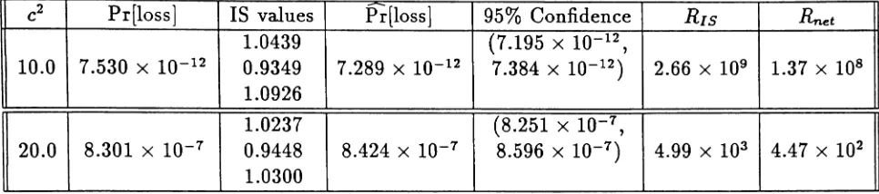
c2 Pr[loss] IS values ~[loss] 95% Confidence RIS

Rnet

1.0439 (7.195

x

10-12_,

10.0 7.530 X 10-1 2 0.9349 7.289 X 10-12 7.384 X 10-12) 2.66 X 109 1.37 X 108

1.0926

1.0237 (8.251

x

10-7_,

20.0 8.301 X 10-7 0.9448 8.424 X 10-7 8.596

x

10-7) 4.99 X 103 4.47 X 102

1.0300

Table 2: Blocking probabilities and speed-up factors using the proposed algorithm for the

IBP /Geo/1/K queue, with {3

==

0.35147, K

==

200. For these estimates: N R

==

100 NRC

=

500.

'

(p

==

0.965048543,q

==

0.976699029,{3

==

0.35147,K

==

200), and (p

==

0.976470588,q

0.984313725,{3

==

0.35147,K

==

200). The threshold Th of Fig. 2 was set to 10-13, 10-8 and

10-6_{, respectively.}

Table 2 summarizes the results, including the near-optimal IS parameters found by MFA, the corresponding estimated blocking probabilities, the estimated confidence intervals and the speed-up factors with respect to conventional MC simulation. For these estimates we used

N R

==

100, NRC

==

500. We estimated Rt

==

19.38 when c2

==

10.0, and R;

==

11.16 when

c2

==

_{20.0. Estimated blocking probabilities are in agreement with the known, analytically}

calculated probabilities, as illustrated in Fig. 10.

7.3

Realistic System:

ATM

Switch

The Asynchronous Transfer Mode (ATM) appears to be the evolving standard for broadband

ISDN. We consider an ATM switch with buffers at the input ports. The switch fabric is a

Clos three-stage interconnection network. For a detailed description of the switch and an

approximate model for its operation see [23] and references within. Such an NL x NL Clos

cell switch is shown in Fig. 11.

The bursty arrival process to each input port is modeled as a discrete time Interrupted Bernoulli Process (IBP), described in the previous segment. For this type of switch an

ap-proximation algorithm was constructed in [23].

Under regenerative/dynamic IS, we choose the times that a cell arrives to an empty buffer and the arrival process has just changed to active, as the regeneration points. Note that this is an approximation, required here due to the impractical length of the "true" regeneration cycles based on all the buffers being empty, and all the arrival processes just changing to

active and producing an arriving cell. Our approximation is supported by the fact that

these approximate RC's (ARC's) are long enough to allow us to consider events across cycles

"practically independent". It is also supported by the extensive experimental correlation

analysis we conducted, i.e., estimates of the correlation existing ARC's were consistent with

our assumption of independence.

Statistical Optimization of Dynamic Importance ... ,M. Devetsikioiis and

J.

K. Townsend 19

~

»:

/

/

I

-/

- -

Exact results

,

-I

II

IS simulation

-I

I

-,

•

1

0.1

~ 0.01

==

0.001

~

0.0001

.c

e

1e-05

~_Of} 1e-06

:i

1e-07

.2

1e-08 ~ 1e-09 1e-10 1e-11 1e-12

10 100

1000

10000

Figure 10: Estimated blocking probabilities and analytically calculated probabilities vs. the squared coefficient of variation, c2, for the IBP /Geo/l/K queue.

2

n

1

2

n+1

2n

N-n+1

N

Statistical Optimization of Dynamic Importance... ,M. Devetsikioiis and J. K. Townsend 20

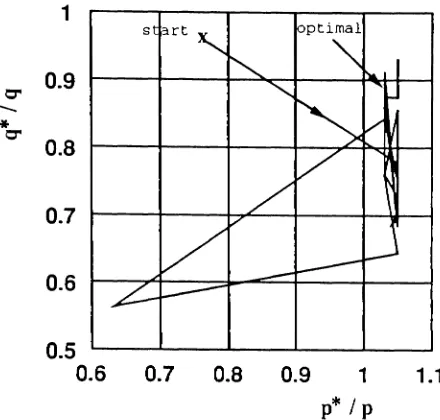
1

s art

0.9

0"'

--*

0"'

0.8

0.7

0.6

0.5

0.6

0.7

0.8

0.9

1 1.1

p" / p

Figure 12: Trajectory of the IS parameters moving towards the near-optimal solution for the

ATM switch model.

model, there is no explicit service probability 1 -

f3

available to be modified. In each ARC,

we bias initially p and q to

pi

and q;, until the weight function (likelihood L*) decreases to a

prespecified minimum, then change IS parameters to

p;

and

q;

in order to empty the queue

and, finally, change to

pi

and

qi

in order to allow fast regeneration.

In our experiments, we set p; == 0.3p,

pi

== p, q; == 1.045q,

qi

== q, and optimized with

respect to the settings of

pi

and

q;

using MFA. The number of input lines was NL == 16,

with input buffers of length

K

== 200 each. In applying MFA we set a1 ==

pi,

a2 ==

qi,

A17la z ,1 == 1.07p, Am i n , l == O.lp, Am a z ,2 == 1.045q, Am i n ,2 == O.lq, I == 0.8, M == 50, E == 5,

N == 100, T_{m a z} == 8.0 X 10-2, and Tmin == 8.0X 10-5• Results were obtained for a configuration

that corresponded to c2 _{== 10.0: (p == 0.932075471,q == 0.954716981,N}

L == 16,K == 200).

Symmetric traffic conditions over the 16input lines were assumed. The threshold Th of Fig. 2

was set to 10-13 •

Fig. 12 shows an example of the trajectory of the IS parameters moving towards the

near-optimal solution for the ATM switch model. Table 3 summarizes the results, including the near-optimal IS parameters found by MFA, the corresponding estimated blocking probability, the estimated confidence interval and the speed-up factor with respect to conventional MC

simulation. For these estimates we used NR == 50, N

nc

== 100. We estimated H, == 25.0.

Statistical Optimization ofDynamic Importance... , M. Devetsikiotis and

J.

K. Townsend 21

Pr[loss] IS values P~[loss] 95

%

Confidence RIS

Rnet

unknown 1.0504 1.93 x 10-10 _{(1.501 X 10-}10

, 4.15 X 106 1.66 X 105

0.8938 2.356 x 10-10₎

Table 3: Blocking probabilities and speed-up factors using the proposed algorithm for the

16 x 16 ATM switch, with p

=

0.932075471, q

=

0.954716981, c2

₌

_{10.0, and K}

₌

_{200. For}

these estimates: N R

==

50, NRC

=

100.

Approx. results

Brute-force

Me

1

0.1

>, 0.01

.a.J

:::: 0.001 ]_eu 0.0001

~ 1e-05

~

1e-06

g

1e-07

~_o 1e-08

~ 1e-09

"' 1e-10 1e-11 1e-12

10

o

II

100

IS simulation

1000

10000

Figure 13: Plot comparing the approximation results with conventional

Me

results (where it

was possible) and the simulation result obtained using IS. Blocking probabilities are plotted

vs. the squared coefficient of variation c2• IS results are consistent with conventional MC

Statistical Optimization of Dynamic Importance... , M. Devetsikiotis and J. K. Townsend 22

Buffer Pr[loss] IS values P~[loss] 95% Confidence RIS

Rnet

K -70 unknown 1.0905 1.042

x

10 9 (6.978 X 10-10_{, 2.63 X 10}4 _{2.17 X 10}3

0.8683 1.381

x

10-9₎

K -

85 unknown 1.0905 2.19

x

10 11 (1.307 X 10-1 1, 8.89 X 105 7.06 X 104

0.8683 3.073

x

10-11

)

Table 4: Low priority cell blocking probabilities and speed-up factors for the 4 x 4 ATM

switch, with p

==

0.908411, q

==

0.960747, c2

==

10.0, and PH

==

0.3. For these estimates:

N

R

==

20, NRC

==

10,000.

7.4

N

_L X

N

_L

ATM Clos Switch with Head-of-Line Priority and

Push-Out

Again, we consider an ATM switch with buffers at the input ports, modeled as a slotted-time

queueing system. Such an N_L

x

N_L Clos cell switch is shown in Fig. 11. Furthermore, we

assume that there exist two classes of cells, high priority and low priority cells, and that

the switch operates with head-of-line priority and push-out. For a detailed description of the

switch and an approximate model for its operation see [24] and references within.

The ATM switch we study here has NL

==

4 input lines, symmetric traffic over

all

input

lines, two classes of cell priority (high and low), average rate of arrival in each line A

==

0.3,

probability that a cell has high priority PH

==

0.3, and buffers of length K

==

70.

A pproximate regeneration cycles (ARC's) were again used, as described in the previous

section.

IS biasing was done dynamically. In each ARC, we biased initially p and q to p~ and q;,

until the weight function (likelihood

L*)

decreased to a prespecified minimum, then changed IS parameters to

p;

and

qi

in order to empty the queue and, finally, changed to

pi

and

q;

in order to allow fast (approximate) regeneration. In our experiments, we set p;

==

p;

==

p,

qi

==

q~

==

q,

PH

==

PH·

We optimized IS performance with respect to the settings of p~ and q; using MFA, in a way similar to [19]. The blocking probability for low priority cells were estimated that corresponded to c2

=

_{10.0: (p}

=

_0.908411,q

=

_0.960747,NL

=

_4,PH

=

_0.3,K

=

_{70). We}

used the same IS values to estimate the blocking probability for c2 = 10.0: (p = 0.908411, q =

0.960747, NL

=

4,PH

=

0.3, K

=

85). This demonstrates a certain robustness of the optimal IS setting with respect to the queueing capacity, when all other coefficients remain fixed. Table 4 summarizes the results. For these estimates we used NR = 20, NRC = 10,000. We

estimated

R;

=

12.1 when

K

=

70, and

R

t

=

12.59 when

K

=

85.

8

Conclusions

Statistical Optimization ofDynamic Importance ... ,M. Devetsikiotis and J. K. Townsend 23

periods can be achieved simultaneously.

In most realistic systems, the IS estimator variance is not known in closed form. For these cases, minimizing statistical estimates of the variance with respect to the IS parameters can be a useful alternative. The SA and MFA optimization algorithms are appealing because of their increased resistance to the noisiness of the cost function and their ability to escape local minima. We have presented a methodology that uses the MFA algorithm in conjunction with statistical estimates of the IS estimator variance, to obtain near-optimal IS parameter settings.

Run time speed-up factors of two to eleven orders of magnitude over conventional MC sim-ulation are obtained using our methodologies for a wide variety of queueing systems, including systems with correlated arrivals and multiple queues.

References

[1] H. Kahn and A. W. Marshall. Methods of Reducing Sample Size in Monte Carlo Com-putations. Opere Res. Soc. of Amer., 1:263-278, Nov. 1953.

[2] K. S. Shanmugan and P. Balaban. A Modified Monte-Carlo Simulation Technique for the Evaluation of Error Rate in Digital Communication Systems. IEEE Trans. Commun.,

COM-28(11):1916-1924, Nov. 1980.

[3] D. Lu and K. Yao. Improved Importance Sampling Technique for Efficient Simulation of Digital Communication Systems. IEEE J. Select. Areas Commun., 6(1), Jan. 1988.

[4] S. Parekh and

J.

Walrand. A Quick Simulation Method for Excessive Backlogs in Net-works of Queues. IEEE Trans. Automat. Contr., AC-34(1):54-66, Jan. 1989.

[5] P. W. Glynn and D. L. Iglehart. Importance Sampling for Stochastic Simulations. Man-agement Science, 35(11):1367-1392, Nov. 1989.

[6]

J.

S. Sadowsky and J. A. Bucklew. On Large Deviation Theory and Asymptotically Efficient Monte Carlo Estimation. IEEE Trans. Inform. Theory, IT-36(3):579-588, May

1990.

[7] V. S. Frost and Q. Wang. Efficient Estimation of Cell Blocking Probability for ATM Systems. In Proc. of IEEE Int. Conf. Commun., Denver, CO, 1991.

[8] M. R. Frater, T. M. Lennon, and B. D. O. Anderson. Optimally Efficient Estimation of the Statistics of Rare Events in Queueing Networks. IEEE Trans. Automat. Contr.,

AC-36(12):1395-1405, Dec. 1991.

[9] A. Goyal, P. Heidelberger, and P. Shahabuddin. Measure Specific Dynamic Importance Sampling for Availability Simulations. In Proc. 1987 Wint. Simul. Conf., pages 351-357,