A Structured Analytical Technique For Technology Evaluation Of Developing Technologies

(1)

ABSTRACT

JAYANTHI, SRIKANTH. A Structured Analytical Technique For Technology Evaluation Of Developing Technologies. (Under the direction of Dr. Robert E. Young.)

Technology Management is a vast area, and is becoming increasingly important in the light of rapid development of future technologies and advanced research in several areas of application. It is important for organizations to monitor various developments and select technologies that best suit their business needs.

Technology Evaluation is one of the areas within technology management that helps in evaluating the potential of new technologies. In this thesis, technology evaluation is the process of evaluating a technology with respect to various performance requirements that it is expected to satisfy. Many relevant techniques that exist are mostly complex, confusing or unsuitable for technology evaluation. Most of the time, expert opinion is used in generating an evaluation report that may not highlight the critical relationships between various factors and the end requirements.

The objective of this thesis is to develop a structured analytical technique for technology evaluation. The purpose of the technique is to help in estimating the suitability of a

technology for a particular set of needs. It also helps in identifying potential problem areas that exist in a technology. The technique basically consists of three levels (1,2 and 3) to relate various parameters and a SWOT analysis to analyze subsystems. For purpose of clarity the technique can be separated into two phases. In the ‘Identification Phase’, the performance requirements, features and subsystems of the technology are identified. Also, weights are assigned (in Levels 2 and 3) to all the parameters to establish the dependency between them. Finally, the ‘Analysis Phase’ involves a SWOT analysis of the various subsystems of the technology. The ratings derived from the SWOT analysis are used in Levels 3, 2 and 1 to estimate the overall performance levels.

(2)

developing ‘smart objects’. Case Study 2 – Fuzzy Configurator System is a research undertaken by Muhammad Neil El Himam, under the direction of Dr. Robert E. Young in Industrial Engineering Department of NC State University. The Fuzzy Configurator System is being developed using fuzzy constraint networks and database technology. The case studies help in bringing out some shortcomings of the technique.

(3)

A STRUCTURED ANALYTICAL TECHNIQUE FOR TECHNOLOGY

EVALUATION OF DEVELOPING TECHNOLOGIES

by

SRIKANTH JAYANTHI

A thesis submitted to the Graduate Faculty of North Carolina State University in partial fulfillment of the requirements for

the Degree of Master of Science

INDUSTRIAL ENGINEERING

Raleigh

2002

APPROVED BY:

MICHAEL G. KAY CECIL C. BOZARTH Co-Chair

(4)

DEDICATION

To all those people who with great integrity and passion have sacrificed their lives for a

(5)

BIOGRAPHY

(6)

ACKNOWLEDGEMENTS

This thesis has been made possible through support of numerous people who have guided me and encouraged me during my work. I am very grateful to Dr. Robert E. Young for his constant guidance and advise in completing this thesis. I am thankful to Dr. Michael G. Kay for his encouragement and support and Dr. Cecil C. Bozarth for being in the committee and supporting this thesis. Special thanks to Muhammad Neil El Himam and Ajith Parlikad for helping me do the case studies in this thesis.

(7)

LIST OF TABLES

Table 1.0 Features Vs Performance requirements ……….. 18

Table 1.1 Illustration of Features Vs Performance requirements in a PC ….. 18

Table 2.0 Subsystems Vs Features ………. 19

Table 2.1 Illustration of Subsystems Vs Features ……….. 20

Table 3.0 Guidelines for assigning Confidence Levels …..……… 23

Table 3.1 SWOT analysis of the CPU system ……… 24

Table 4.0 Case Study 1 - Matrix of Performance Requirement Vs Features . 40 Table 4.1 Case Study 1 - Matrix of Features Vs Subsystems ……… 41

Table 4.2 Case Study 1 – Performance Evaluation of Auto-ID Technology 52 Table 5.0 Case Study 2 – Matrix of Performance Requirement Vs Features 59 Table 5.1 Case Study 2 – Matrix of Features Vs Subsystems ……… 60

(11)

LIST OF FIGURES

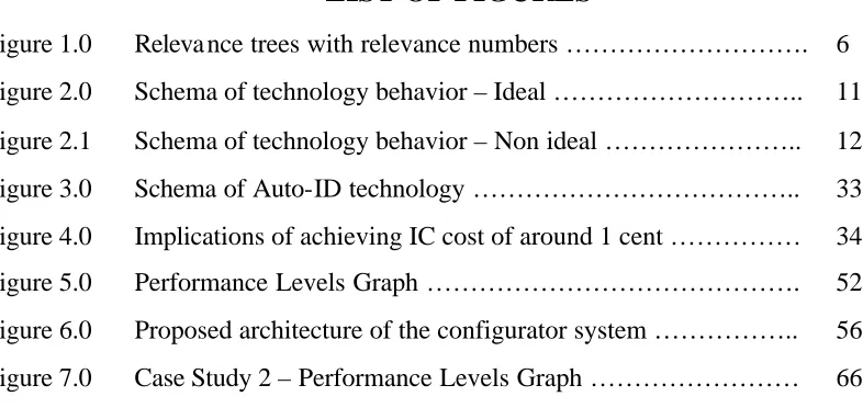
Figure 1.0 Releva nce trees with relevance numbers ………. 6

Figure 2.0 Schema of technology behavior – Ideal ……….. 11

Figure 2.1 Schema of technology behavior – Non ideal ……….. 12

Figure 3.0 Schema of Auto-ID technology ……….. 33

Figure 4.0 Implications of achieving IC cost of around 1 cent ……… 34

Figure 5.0 Performance Levels Graph ………. 52

Figure 6.0 Proposed architecture of the configurator system ……….. 56

(12)

GLOSSARY

Critical Elements: Positive or negative elements that are most important and either decide the success or failure of the working of a system.

Elements of a System: Element of a system may be a characteristic, a technical detail, a forecast, or any other point related to the system which can be used in its analysis.

Major Elements: If positive, they are elements that are important and enhance the working to a great extent. If negative, they are elements that may cripple the working of a system.

Minor Elements: If positive, they are elements that are of less importance but may contribute positively in the long run. If negative, they are elements that may cause inconvenience during the working of the system.

Technology Analysis: Task of analyzing technologies that are relevant for competition and the company’s position in these areas [2].

Technology Monitoring: Observation of technologies and research results that already exist (‘state of the art’).

Technology Prognosis: Task of developing statements on future trends of science and technology.

(13)

“Not everything that can be counted counts, and not everything that counts can be counted”

– Albert Einstein.

1.0 INTRODUCTION

1.1 Overview

The world is witnessing an unprecedented change in technological advances. At any given time there are numerous technology developments happening concurrently around the world. Of these, some may have the potential to change the way we live our lives. Many companies and research establishments are making efforts to stay abreast of the latest developments in relevant fie lds. There is a general agreement about the need for a technology foresight among companies though the effort and resources put into this activity may vary considerably [2]. The reasons for doing this maybe one of the following:

• To evaluate the feasibility of developing, commercializing and doing business in the new technology, or,

• To evaluate the utility of the new technology for improving the efficiency of business systems and stay ahead of competition.

The manifestation of technology can range from just a piece of knowledge for a method or technique, all the way to a complex system of machinery and its inherent intelligence [4]. There are many definitions of technology and distinctly different elements from physical to cultural may appear in them [10]. It is best to define a technology from the context of its usage. In this thesis, technology may be considered as a complex system consisting of multiple subsystems working in coordination to achieve certain needs.

(14)

Technology forecast involves predicting the path that a technology may take in a given time frame based on the available data and expert opinions. It may be very difficult to predict the trends that a technology may follow because of the socioeconomic process involved in the development. Though some analyses are highly mathematical and sophisticated, they have largely failed to deliver in their purpose [5].

Technology foresight is said to be oriented towards systematic recognition and observation of new technologies or existing technologies, the evaluation of their potential and their

importance for the competitiveness of the organization, and storing and diffusion of

information. Technology foresight includes the process of technology analysis, technology monitoring, technology prognosis and technology scanning [2].

Technology management, over the years, has evolved to encompass a broad range of knowledge and practice dealing with managing technology in an organization. Technology management can be considered as the broad umbrella under which all techniques, tools and activities discussed in this thesis including technology evaluation would fall.

The focus of this thesis is on evaluating the potential of a technology to satisfy the needs for which the technology may be deployed. Also, in doing so, the strengths and weaknesses of the technology are brought into perspective. This task is called “Technology evaluation”. Technology evaluation is performed in any situation that requires an insight into a

technology before it can be taken up for the intended purpose. Technology evaluation also is an important part of technology forecast and technology foresight.

(15)

with the application needs. Moreover, it will be difficult to understand the effect of certain known strengths and weakness in the technology on the performance expectations.

The main purpose of this thesis is to develop a technique in which a technology can be evaluated from the perspective of satisfying the performance needs. The technique is intended to be a balance of subjective and objective analysis without being too comple x to comprehend. Also the technique would aid in any decision-making process. Two case studies of developing technologies are made to understand the applicability and usefulness of the technique.

1.2 Existing tools and techniques

There are different tools and techniques used in technology management. The tools range from being simple to highly mathematical with sophisticated analyses. Each technique is intended towards a particular activity within technology management. A few of the

techniques are briefly described in this section. These techniques are mentioned because of either of the following reasons:

a. They are widely known in the field of technology management.

b. They somewhat resemble the technique in this thesis but are not suitable to be applied for technology evaluation.

1.2.1 Analytical Hierarchy Process (AHP)

AHP is an effective tool for a complex decision- making process by comparing multiple alternatives for a given problem or goal [20]. The method weighs the importance of factors that are critical to meet the goal and then compares alternative solutions against these factors. Using matrices at different decision levels, pair-wise comparison of alternatives is made by assigning relative importance weights.

(16)

• It does not provide for a systematic analysis of the content or the inherent characteristics of a technology.

• It is not suitable for an absolute evaluation of a technology since the method is oriented towards relative comparison among alternative solutions.

1.2.2 Quality Function Deployment (QFD)

QFD is a technique to ensure that the design and manufacturing of a product conforms to the end user requirements. It also ensures that quality is maintained at each stage of product development [6]. QFD works with different levels using matrices. It is a top down approach where matrices are used to convert customer requirements into measurable design and

manufacturing specifications. QFD also helps in prioritizing requirements and benchmarking competition.

Although QFD finds its main application in product deve lopment, it has been modified suitably and used in various other areas like service industries, education and fields such as Business Process Reengineering, Failure Mode Effects Analysis, Situation Analysis and more7.

The shortcomings of QFD for technology evaluation are:

• The technique does not provide to move ratings from the bottom levels to upper levels. It is difficult to do a two-way propagation of information. The approach is limited to top down flow of information.

• It does not provide for analysis of actual content of a system if this technique were to be used for technology evaluation.

1.2.3 Design Structure Matrix (DSM)

(17)

The main purpose of DSM is to identify the elements with strong inter-relationships and group them together for better management of the process. DSM can be used to manage product architectures, process flows, and organizational structures.

The shortcomings of DSM for technology evaluation are:

• It is not intended as a goal or objective oriented analysis and not suitable for technology evaluation.

• It works with a single level matrix and hence difficult to represent different levels in a

complex system.

1.2.4 Delphi Technique

Delphi technique is widely used as a group problem solving technique [9]. The identifiable characteristic of this technique is that the participants are isolated from each other and a ‘moderator’ ensures the working of the process. Also, it is an iterative process wherein questionnaires are given to participants during each iteration and only the majority opinions are compiled together for the next iteration. The participants refine or review their opinions till a consensus is reached.

Delphi technique finds its application in numerous areas where expert or group opinion is solicited to arrive at a decision. This technique is used quiet often in technology forecasting.

The shortcomings of Delphi Technique for technology evaluation are:

• The process can lead to a very biased evaluation.

• It is based mainly on opinions and therefore may not have any objective or structured analysis.

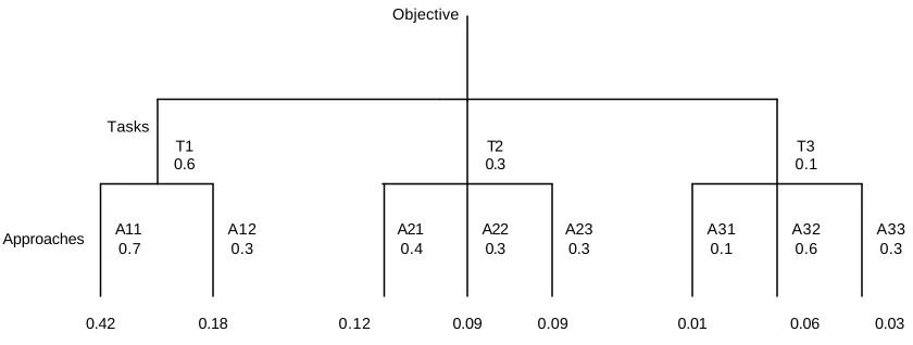
1.2.5 Relevance Trees

(18)

branches out from a starting node that is usually the objective. Branches may represent either a problem or a solution and nodes represent an item. Relevance numbers (normalized at each level) may be given to the branches to indicate its importance towards the objective (see figure 1).

0.03 A33 0.3 Approaches

0.42 0.18 0.12 0.09 0.09 0.01 0.06

A11 0.7 A12 0.3 A21 0.4 A22 0.3 A23 0.3 A31 0.1 A32 0.6 T1 0.6 T2 0.3 T3 0.1 Objective Tasks

Figure 1. Relevance trees with relevance numbers.

Relevance trees are useful in the construction of scenarios and technology forecasts.

The shortcomings of Relevance Trees for technology evaluation are:

• A branch cannot be linked to multiple parent nodes that makes it difficult to represent a problem or solution that can affect more than one parent item.

• The technique does not provide for assigning ratings but only weights for importance.

• Multiple objectives and multiple branches can make the tree complex and huge.

1.3 Conclusion

There are many more techniques present in the field of technology management that are intended for different tasks. Most of the techniques in technology foresight or technology forecast are intended to look towards the future. Some common disadvantages with many of the techniques in technology management are:

(19)

• They ignore the actual facts that count towards evaluation.

(20)

2.0 RESEARCH OBJECTIVES

It is very difficult to completely assess a complex system with only quantitative measures. There will be several elements in the system that critically affect performance and can be represented only in qualitative terms. The effects of these are best understood only by a logical and structured evaluation.

Little work has been done to formalize technology evaluation as a separate area of study in technology management. The task is undertaken on a need basis depending on the situation. As such, there are no standard techniques or tools defined for this purpose. Some

organizations use their own customized approach to do technology evaluation [12]. This thesis proposes to develop a technique that is designed specifically for technology evaluation.

Technology evaluation can range from being simple to a mathematically complex and challenging task. The tasks can vary from gathering expert opinion on a system to assessing socio-economic impact and from gauging the behavior of the system to projecting the financial benefits for the next 10- year period. The evaluation technique in this thesis is focused more towards the overall performance, and factors that impact the performance of the technology. Socio-economic and financial aspects are not taken into account unless they form a significant barrier in achieving an identified performance requirement.

The technique is intended to have the following characteristics. These characteristics help in addressing many of the issues discussed in the previous chapter:

1. Structured analysis.

(21)

2. Easy to comprehend.

The technique in this thesis is designed to be straight forward in its approach. It involves basic level mathematics to assign appropriate weights and ratings. It consists of two clear broad phases. The first phase involves identifying the critical parameters and their

dependence with each other. The second phase involves analyzing the subsystems and assigning ratings. The steps involved in using the technique are explained in chapter 3.

3. Mix of subjective and objective analysis taking into account known facts. It is very difficult to completely eliminate subjectivity in technology evaluation. This is because for many outcomes there may not be a valid and reliable quantitative measure. Even more, the extent to which one believes the usefulness of a quantitative measure in a particular instance is also a matter of judgment [13]. In this technique there is a degree of subjectivity involved in identifying the relationship between the performance

requirements, features and subsystems. But the technique to an extent nullifies the subjectivity by taking into account critical known facts for the evaluation that are likely to have an effect on the performance.

As in most other techniques in technology management, weights and ratings are used in this technique. But the most significant difference here is that the ratings are assigned objectively (as will be shown in chapter 3) to the subsystems. This is not the case in most other techniques since ratings are mainly based on opinions. The final results of the evaluation are shown as percentage performance levels of the technology against each performance requirement.

4. Flexibility in the extent of usage.

Another important advantage of the technique is that the extent of evalua tion can be varied according to the need. In other words, the technique could be used as a quick and dirty tool as well as a framework for an in-depth analysis. Confidence levels are

(22)

that area for a more precise evaluation. Generally, a more detailed study would lead to a more accurate evaluation and a better estimate of the technology behavior.

(23)

3.0 TECHNIQUE FOR TECHNOLOGY EVALUATION

3.1 Overview of the technique

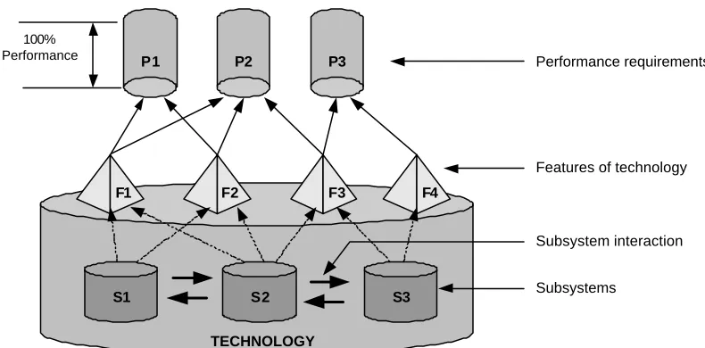
Evaluation of any technology is best done from the viewpoint of the needs that it is expected to satisfy. The performance of technology will mainly depend on the subsystem or the content that it is made up of. These subsystems enable the features of the technology. Therefore it is critical to recognize the dependence between each performance requirement to each feature and in turn each feature with each sub-system of the technology. This forms the basic framework of the technique.

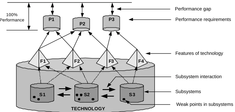
Figure 2.1 shows an ideal situation where subsystems are working perfectly to enable the features and meet the performance requireme nts to a 100% satisfaction. The arrows show the dependence between different components. Any subsystem that is inherently weak or strong will eventually lead to poor or better performance of one or more performance requirements. Figure 2.2 shows the non- ideal situation where the subsystems have weak points and hence the performance is less than 100%.

S3 S2

S1

F1 F2 F3 F4

TECHNOLOGY

P1 P2 P3 Performance requirements

Features of technology

Subsystems

Subsystem interaction

Figure 2.0 Schema of technology behavior - Ideal

(24)

S3 S2

S1

F1 F2 F3 F4

TECHNOLOGY P1

P2 P3 Performance requirements

Features of technology

Subsystems

Subsystem interaction

100% Performance

Weak points in subsystems

Figure 2.1 Schema of technology behavior - Non-ideal

Performance gap

The identification of performance requirements, features and subsystems may take some effort since it is often difficult to clearly distinguish them. A fairly precise identification will lead to a fairly good evaluation. Answering questions of ‘what’ with ‘how’ is used to help in identifying the parameters and establishing dependency between the m. This is very similar to the QFD technique used to ensure quality in product design.

‘Performance requirements’ may vary considerably depending on the case. It is mostly expressed in qualitative terms. For example ‘Quick check-out time at a grocery store’ is a performance requirement for a grocery store system. It is not necessary to set any

(25)

‘Features’ are directly related to the technology. Features are usually the functional aspects of technology. For example, ‘power steering’ is a feature of an automobile.

‘Subsystems’ are in itself a fairly complex integration of different components working towards a common function. For example the ‘CPU’ is a subsystem of a computer. It is necessary to identify the required important subsystems for the purpose of evaluation that are part of the technology.

3.1.1 SWOT (Strengths, Weaknesses, Opportunities, Threats) Analysis

SWOT analysis is a major part of the evaluation technique. It is one of the simple and effective management tools. It is most popular as a tool for top- level management decisions like organizational and marketing strategy. SWOT analysis is chosen since it provides a good framework for studying a topic from different perspectives. It is often used together with other analytical techniques in an analysis [14]. SWOT analysis involves grouping of elements identified as strengths, weaknesses, opportunities or threats.

• ‘Strengths’ are positive elements related to the system and may directly or indirectly

affect the performance. (E.g. ‘Development of high speed web servers’ is a Strength for Internet technology).

• ‘Weaknesses’ are negative elements related to the system and may directly or indirectly affect the performance. (E.g. ‘High energy requirement drains batteries very quickly’ is a weakness in digital cameras).

• ‘Opportunities’ are external and unrelated to the system but support its functioning or

development. (E.g. ‘Development of internet’ is a major opportunity for improved bank ing systems).

(26)

The elements identified in the analysis may not necessarily be purely technical aspects of the system. They could be somewhat abstract in determining the performance of the technology. This is clear with the examples below:

Example 1: ‘Rapid rate of advancement in microprocessors’ in a CPU is a positive factor. The improvements in processors would ensure high processing speeds to keep up with complex software.

Example 2: ‘Very low thermal conductivity of silica’ helps in thermal insulation of a space shuttle during re-entry.

Example 1 is more abstract, but the outlook of the technology in that area of performance is very good. Hence it is important and used in the evaluation. Example 2 is purely technical and can be more directly related to the performance. It is this ability to relate both abstract and direct elements to technology evaluation which makes this technique unique and useful.

3.2 Using the technique

Before using the technique it is helpful to define the technology to be evaluated. The definition will help in providing scope for the evaluation. The technique is explained by using a simple illustration. The evaluation of a Personal Computer system is used as an illustration along with the steps of the technique.

A Personal Computer or a PC is a stand alone computing machine consisting of a monitor,

keyboard, mouse, speakers, a central processing unit, hard disk, memory, input/output ports

and essential software.

(27)

Level 2 is a matrix of ‘Features’ Vs ‘Performance requirements’, with features row wise and performance requirements column wise.

Level 3 is a matrix of ‘Subsystems’ Vs ‘Features’, with subsystems row wise and features column wise.

SWOT analysis is used to analyze subsystems and arrive at overall rating.

As mentioned earlier, for clarity, the technique can be divided into two broad phases:

1) Identification phase. This phase involves identifying the performance requirements, features and subsystems, and establishing the dependence between them by assigning weights. The first 4 steps of the evaluation process is the identification phase.

2) Analysis phase. This phase involves analyzing the subsystems using the SWOT analysis and rating the subsystem. The ratings are later used in the matrices (levels 1, 2 and 3) to arrive at the performance levels of the requirements. Step 5 and 6 of the evaluation process is the analysis phase.

The different steps in using the technique are explained below:

Step 1: Identification of performance requirements.

To begin with, the performance requirements that the technology is intended to satisfy are identified.

Illustration

The performance requirements expected out of a Personal Computer (PC) system are:

1. Ability to perform the required task effectively.

2. Convenient input interface to the computer.

3. Convenient output interface from the computer.

(28)

5. Store data reliably for access.

Step 2: Identification of features of the technology.

The features identified should be particularly helpful in meeting the performance requirements.

Illustration

The features of a PC system are:

1. Ability to run different software for performing required tasks.

2. Peripherals like keyboard and mouse for data entry and input control.

3. Continuous visual display of information through the monitor.

4. High speed processing of data.

5. Hard disk storage of data in the form of files and folders.

6. Compatible to connect to other external equipment like printer, scanner, etc.

Step 3: Identification of the subsystems in the technology.

The subsystems should support all the features mentioned in step 2. As far as possible the subsystems should be clearly separable parts of the technology. It may be better to define the scope of each subsystem for eliminating ambiguity.

Illustration

The subsystems of a PC are given below.

1. CPU (Central Processing Unit)

The CPU is made up of the microprocessor that acts like the brain of the computer.

For the purpose of evaluation, the serial and parallel ports and other sockets are

considered to be part of CPU. The CPU does all the data processing work for the

computer and is one of the most important components of a PC.

(29)

The output system consists of all the peripherals that show output to the user. Mainly

these are monitor and printer. Other output devices are speakers, headphones, etc.

3. Input system

The input system mainly consists of the keyboard and mouse. Other input equipment

can be scanner, microphone, etc.

4. Hard disk and memory

The hard disk stores all the data in the computer. Apart from the local hard disk,

portable disks like the floppy and zip disk are also used to store data. Memory is the

RAM (Random Access Memory), which is used to store data temporarily during the

working of the computer.

5. Operating system

Operating system is the software, which controls the use and interaction of hardware

and applications of a computer.

Step 4: Assigning weights to establish dependence between performance requirements with features and features with subsystems.

a. Comparing performance requirements with features:

For every performance requirement R, weights W are assigned corresponding to each feature indicating extent of effect the feature has on the requirement. The sum of the weights given to the features for each performance requirement should total to 1. (See Table 1.0)

Let Wij be the weight assigned for every ith feature and jth performance requirement. Then

1

1 =

∑

= N

i j

W where N is the number of features identified and j = 1, …, M are the number of

(30)

Performance Requirements Features

R1 R2 … RM

F1 W11 W12 … W1M

F2 W21 W22 … W2M

… … … … …

FN WN1 … … WNM

Total 1 1 1

Table 1.0 Features Vs Performance requirements.

Illustration

PC system.

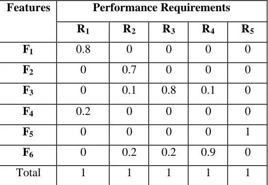
Weights assigned for ‘Features Vs Performance requirements’ are shown in Table 1.1.

In the table there are N = 6 features and M = 5 requirements.

Performance Requirements Features

R1 R2 R3 R4 R5

F1 0.8 0 0 0 0

F2 0 0.7 0 0 0

F3 0 0.1 0.8 0.1 0

F4 0.2 0 0 0 0

F5 0 0 0 0 1

F6 0 0.2 0.2 0.9 0

Total 1 1 1 1 1

Table 1.1. Illustration of ‘Features Vs Performance requirements’ in a PC.

For sample, weights against requirement R1 are explained.

R1 = Ability to perform the required task effectively.

F1 = Ability to run different software to perform the required task.

(31)

The tasks that need to be performed using a computer can be various and a single software

cannot support all the needs. Hence the ability to install different software on a computer

will have the most effect in satisfying this requirement. Therefore this is given a weight of

0.8. High speed processing helps in performing complex tasks quickly and efficiently. But

this is of less effect for the requirement compared to F1. Hence a weight of 0.2 is given. The

other features do not contribute to the requirement (at least not directly), therefore have zero

weights for R1.

To help in this process it is always better to be able to think of reasons while assigning weights.

b. Comparing features with subsystems.

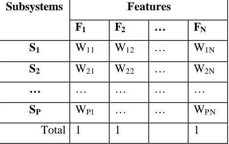
For every feature F, weights W are assigned corresponding to each subsystem S, indicating the proportion of dependence of the feature on each subsystem. The sum of the weights given to the subsystems for each feature should total to 1. (See Table 2.0)

Let Wki be the weight assigned for every kth subsystem and ith feature. Then 1

1 =

∑

= P

k i

W where

P is the number of subsystems identified.

Features Subsystems

F1 F2 … FN

S1 W11 W12 … W1N

S2 W21 W22 … W2N

… … … … …

SP WP1 … … WPN

Total 1 1 1

(32)

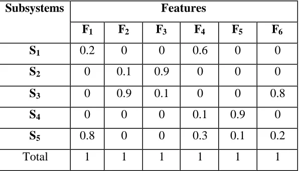
Illustration

PC system.

Weights assigned for ‘Subsystems Vs Features’.

In the table there are N=6 features and P=5 subsystems.

Features Subsystems

F1 F2 F3 F4 F5 F6

S1 0.2 0 0 0.6 0 0

S2 0 0.1 0.9 0 0 0

S3 0 0.9 0.1 0 0 0.8

S4 0 0 0 0.1 0.9 0

S5 0.8 0 0 0.3 0.1 0.2

Total 1 1 1 1 1 1

Table 2.1 Illustration of ‘Subsystems Vs Features.’

For sample, weights against feature F4 is explained:

F4 = High speed processing of data.

S1 = CPU or Central Processing Unit.

S4 = Hard drive and memory.

S5 = Operating system.

The feature F4 depends on the strengths of three subsystems S1, S4 and S5. The speed of a

microprocessor in a CPU is a major factor in ensuring fast processing of data. Therefore

this is assigned a weight of 0.6. Operating systems that cannot handle multiple tasking well

or if the version is outdated to optimally support applications, this will affect the processing

of data. This takes the next importance after CPU and hence assigned a weight of 0.3. The

memory or the RAM of a computer should be sizable enough to handle movement of data

between the applications and the CPU, else low memory will lead to slow computing. This is

(33)

Step 5: Analyzing subsystems using SWOT method.

The SWOT method is further enhanced in this technique to provide assigning points to the elements of a subsystem. This is used finally to calculate the overall rating of the subsystem. The ratings range from 0-12 with 12 being a perfect system. An important assumption here is that a subsystem is neutral (6 rating), unless determined with facts that it is above average or below average. In other words elements identified in the SWOT analysis prove that the subsystem is above average or below average. Therefore, a more detailed study will lead to a more precise evaluation.

The steps below in conjunction with Appendix 1 show the sequence of analysis –

1. Identification of elements of the subsystem based on the study and grouping them as strength, weakness, opportunity or threat.

Strengths and weaknesses are internal to the system. Opportunities and threats are external to the system.

2. Identification of importance of the element as either ‘critical’, ‘major’, or ‘minor’ (see definition in nomenclature) and assigning points according to the table below.

Classification Points

Minor ±_{0 to 3} Major ±_{0 to 6} Critical ±_{0 to 9}

Points are given to elements depending on their contribution to the system. An element classified as minor can get a maximum of 3 points. Likewise a major

(34)

If the element is a Strength or an Opportunity then it is assigned positive points. On the other hand if the element is a weakness or a threat it is assigned negative points.

3. Calculate the overall rating of the subsystem as below and assign a confidence level. As mentioned earlier, the initial rating of the subsystem starts with 6. The element points are used to determine the remaining 6 units in the overall rating on a 0-12 scale.

Initial rating of the system = 6

Maximum points (element points) possible, M:

M = No. of critical elements*9 + No. of major elements*6 + No. of minor elements*3

Total points (element points) assigned after analysis, G:

G = Sum of critical points assigned + Sum of major points assigned + Sum of minor assigned

Rating per point = [12 – Initial rating of the system]/ M

Overall rating = Initial rating + Rating per point * G

Confidence level of assessment = C

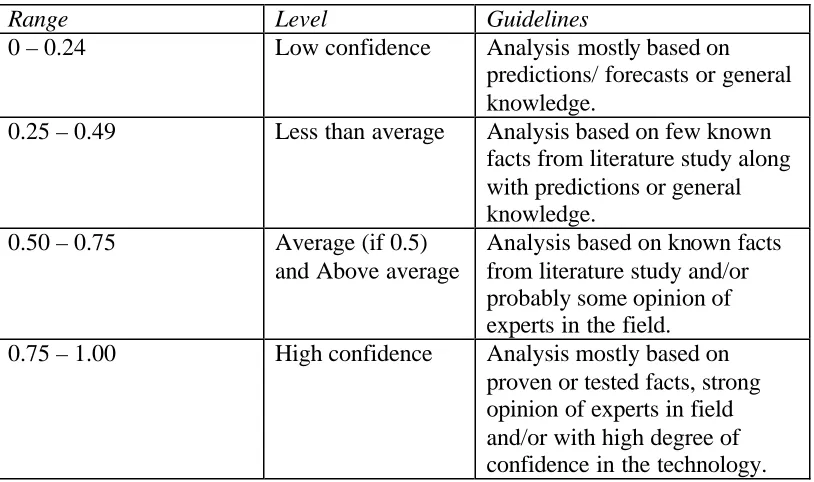
3.2.1 Confidence Levels

(35)

Range Level Guidelines

0 – 0.24 Low confidence Analysis mostly based on predictions/ forecasts or general knowledge.

0.25 – 0.49 Less than average Analysis based on few known facts from literature study along with predictions or general knowledge.

0.50 – 0.75 Average (if 0.5) and Above average

Analysis based on known facts from literature study and/or probably some opinion of experts in the field. 0.75 – 1.00 High confidence Analysis mostly based on

proven or tested facts, strong opinion of experts in field and/or with high degree of confidence in the technology. Table 3.0 Guidelines for assigning confidence levels

3.2.2 Identifying Strengths, Weaknesses, Opportunities, Threats

Some guidelines for identifying Strengths, Weaknesses, Opportunities and Threats are given below. But the analysis is not limited to these guidelines. Any element that falls outside these guidelines can also be included for evaluation.

Strengths

• Salient features of the subsystem.

• Rate of advancement in the technology.

• Life cycle of the system/technology (positive if it is long).

• Cost of implementation (positive if it is affordable). Weaknesses

• Technical implementation barriers.

• Weak features of the system.

• Life cycle of the system/technology (negative if it becomes obsolete soon).

• Cost of implementation (negative if it is high).

Opportunities

(36)

• Infrastructure advantages.

• Integration with other subsystems (positive if it is compatible). Threats

• Alternative systems (current or in-development).

• Infrastructure advantages.

• Integration with other subsystems (negative if there is incompatibility).

Illustration

PC System

The rating given to one of the PC subsystem - ‘CPU’ is shown below. The rating for other

subsystems is given in Appendix 3.0, 3.1, 3.2 and 3.3.

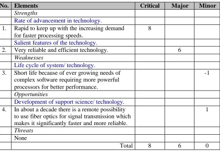
SWOT analysis of CPU system Points: +/- 0 to 9 +/- 0 to 6 +/- 0 to 3

No. Elements Critical Major Minor

Strengths

Rate of advancement in technology.

1. Rapid to keep up with the increasing demand for faster processing speeds.

8

Salient features of the technology.

2. Very reliable and efficient technology. 6

Weaknesses

Life cycle of system/ technology.

3. Short life because of ever growing needs of complex software requiring more powerful processors for better performance.

-1

Opportunities

Development of support science/ technology. 4. In about a decade there is a remote possibility

to use fiber optics for signal transmission which makes it significantly faster and more reliable.

1

Threats

None

Total 8 6 0

(37)

Calculations:

Initial rating of the system = 6

Maximum points (element points) possible, M: No. of critical elements = 1

No. of major elements = 1 No. of minor elements = 2 Therefore M = 1*9 + 1*6 + 2*3

= 21

Total points (element points) assigned after analysis, G: Sum of critical points assigned = 8

Sum of major points assigned = 6

Sum of minor points assigned = -1 + 1 = 0 Therefore, G = 8 + 6 + 0

= 14

Rating per point = [12 – Initial rating of the system] / M = [12 – 6] / 21

= 0.2857

Overall rating = Initial rating + Rating per point * G = 6 + 0.2857 * 14

= 10.00

Confidence level of assessment, C = 0.5 (Average confidence level is given since the CPU system is an existing technology and the analysis is based on certain experienced and known facts.)

Step 6: Evaluation of performance levels by using subsystem ratings.

The ratings calculated in step 5 are used in level 3 (Subsystems Vs Features). The points below in conjunction with Appendix 4 show the matrix calculations.

• The overall ratings from step 5 are moved to the column, ‘Ratings’ corresponding to

each subsystem.

(Also, the confidence levels are moved corresponding to each subsystem. The confidence levels are shown in italics in alternative rows.)

(38)

(The confidence level for each subsystem against each feature = CL * Weight. The total confidence level for each feature is sum of confidence levels in RW column corresponding to each feature.)

• The total rating of each feature is the n moved to level 2 in the column ‘Ratings’ corresponding to each feature.

(Similarly, the total confidence level for each feature is moved to level 2 in the column ‘Ratings’, corresponding to each feature.)

• For each feature against each performance requirement, RW = Rating * Weight. The final rating for each performance requirement is the sum of RW column

corresponding to each performance requirement.

(The confidence level for each feature against each performance requirement = CL * Weight. The total confidence level for each performance requirement is sum of confidence levels in RW column corresponding to each performance requirement.)

• The final rating is then moved to level 1 and is classified as Excellent (if rating > 8 but <=12), Average (if rating > 4 but <=8) or Poor (if rating >4). The final ratings are shown as percentage performance with a graph.

(The total confidence level for each performance requirement is also shown in level 1.)

Illustration

PC System.

(39)

Subsystem Overall rating Confidence level

CPU 10.00 0.5

Output system 6.80 0.4

Input system 9.50 0.5

Hard disk and memory 9.67 0.5

Operating system 7.43 0.4

The ratings and confidence levels are taken into the level 3 as explained in step 6. Level 1

gives the final rating of each performance requirement and the confidence levels against

them.

Appendix 4.1 gives the levels 1, 2 and 3 for the PC System.

3.3 Results and interpretation

The evaluation is done mostly with the performance requirements as the objective. As such the final results show the levels of performance that can be expected from the technology in satisfying these requirements.

The results can be seen in two ways:

1. The final rating of the performance requirements classified as ‘Excellent’, ‘Average’ and ‘Poor’.

(40)

Generally there is very little possibility that the final rating for a performance

requirement is 12. Since, this would mean that one or more subsystems also have a rating of 12 in the SWOT analysis. A 12 rating would mean a perfect system and this is rarely possible. On the other hand a rating of 0 would mean a complete failure to meet the performance requirement. When a reasonable amount of study is made on the technology the rating will surely fall somewhere between 0 and 12.

2. The final ratings shown as percentage performance levels with a graph.

Less than 100% signifies that there are elements in the analysis that are either not completely satisfactory and/or elements that negatively affect the performance of the technology. Lesser the percentage, greater the bad elements in the evaluation. The causes can be traced back with the help of weights given in the matrices to find out the significant elements that affect the performance levels. A comparison of all the

performance requirements with the graph shows which requirement is best met by the technology.

In the present form it would not be possible for the technique to show the performance level with a unit of measurement. For example if the requirement is ‘Speed of 100 mph’, the technique may give an expected performance of 70% against this requirement instead of giving a measure in ‘mph’. The lack of 30% is because there are reasons to believe that the technology is not completely perfect and would not deliver the results 100% of the time.

The confidence levels shown in level 1 signify the confidence in assessment. The confidence levels are propagated similar to the ratings from the SWOT analysis. A lesser confidence level shows that more depth of study may be necessary to further refine the evaluation.

(41)

Results and Interpretation of the PC system

The result of the PC system evaluation is shown in Level 1 of Appendix 4.1. The graph shows

the percentage performance of each requirement.

The final ratings and confidence levels are summarized below –

Performance requirement Final rating Confidence level

R1 8.19 (Excellent) 0.43

R2 8.80 (Excellent) 0.41

R3 7.30 (Average) 0.41

R4 8.09 (Excellent) 0.43

R5 9.44 (Excellent) 0.49

The results show that the performance requirement R3 (‘Convenient output interface’), is the

only one classified as average. Also we can infer that R5 (‘Store data reliably for easy

access’) is the requirement which the PC satisfies best.

Overall the requirement of ‘Convenient output interface’ from a personal computer has

somewhat less performance compared to other requirements that is expected from a personal

computer. With the help of weights given, we can map this low performance to causes such

as problems in monitors and printers.

The PC system was used only to illustrate the technique. Hence, a detailed study was not

made and most of the analysis was based on a few known facts. As such we see that the final

confidence levels are in the less than average level.

3.4 Summary

(42)

4.0 VALIDATION OF THE TECHNIQUE

Validation in the context of this thesis although cannot be proved as in a mathematical theorem, can best be emphasized by the principle, concept, logical structure and assumptions behind the technique. The case studies illustrated in this thesis help in demonstrating the utility of the technique.

4.1 Principle and concept

It is essential to understand a technology in the context of its uses and not just by its technical content or existence [4]. As such an evaluation of a technology cannot be made in isolation from its purpose. This evaluation technique starts with a focus on the requirements expected to be met by the technology and then tries to answer the question ‘how’ leading to an

analysis of various subsystems. As such the evaluation is effective without losing sight of the purpose of the technology. The concept of answering ‘what’ and ‘how’ in the matrices used in this technique is similar to the Quality Function Deployment (QFD) that has shown its effectiveness in ensuring quality in product design.

4.2 Structure

The technique is intended to streamline the knowledge about the technology and structure it in a way so as to understand the effects on the performance requirements. The weights assigned at different levels establish dependency between different parameters and build the structure. This forms an abstract representation of the structure of the technology. The ratings when propagated through this structure will result in a meaningful analysis of the impact on the performance requirements.

4.3 Assumption in SWOT analysis

(43)

analysis is made with an assumption that unless otherwise proven with facts that support positive or negative effects, the subsystem is said to have an average performance. The analysis is designed to reduce subjectivity to a good extent. A more detailed study of the technology would lead to a more refined analysis and evaluation.

4.4 SWOT analysis and points

Points assigned to the elements of subsystem help in identifying the importance and also impact that they may have on the final performance. These points are normalized with the 12-scale rating to calculate an overall rating for the subsystems. The scale of points awarded in the SWOT analysis is a matter of convenience and can be altered to increase or decrease the gain.

4.5 Summary

(44)

5.0 CASE STUDIES

The analysis of a technology is based on literature available from different sources and some fairly rough estimates where things are not certain or known. This type of estimate would be necessary for any evaluation undertaken outside the domain of the research organization. Therefore one may expect to see some assumptions in the analysis.

The case studies begin with an overview of the technology along with the issues related to it. Then, evaluation is made using the technique.

5.1 Case Study 1: Automatic Identification Technology (Auto-ID)

5.1.1 Overview

There is extensive research being done in various research centers to extend the applicability of Automatic Identification technology. The evaluation in this case study is based on the research at Auto-ID center of Massachusetts Institute of Technology. Most of the literature for this case study is obtained from publicly available white papers at www.autoidcenter.org. Limited discussion in some areas of research is due to unavailability of details from the research center for confidential reasons. There is continuous development happening at this research center at the time of this writing. Therefore one may expect to see changes from the time this evaluation was made.

The research is focused on developing the technology and infrastructure needed to connect all the physical objects to the information network. The possibility of identifying, tracking and providing intelligence to the physical objects through the information network opens a wide array of applications especially in the area of supply chain systems. This technology may have the potential to deliver significant benefits in several areas of application.

(45)

• RFID Tag (transponder)

• RFID Reader (interrogator)

• Electronic Product Code (EPC)

• Object Name Service (ONS)

• Physical Markup Language (PML)

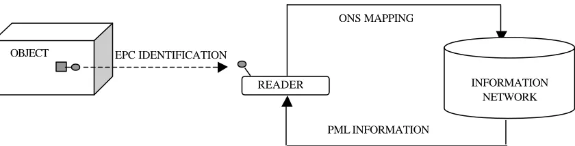
Tags attached to physical objects carry the identification of the object. The identification is in the form of an Electronic Product Code (EPC) that is read by a Reader. Using Object Name Service (ONS), the Reader maps the EPC of the object to a location in the information network containing the information about the object. The information stored in the form of Product Markup Language (PML) is then sent to the Reader to be able to do the necessary action. This is the basic functioning of the technology.

Figure 3.0: Schema of Auto-ID technology.

5.1.1.1 RFID (Radio Frequency Identification) Tag

The radio frequency tag has four components to enable its functionality [15]: 1. IC

2. Antenna

3. Connection between antenna and IC 4. Substrate on which the antenna resides.

PML INFORMATION ONS MAPPING

INFORMATION NETWORK READER

(46)

The target cost for a tag to be economical for large-scale implementation is less than 5 cents. Therefore each of the components listed above should cost around 1 cent. The most

important challenge is in the design and manufacture of IC chip to achieve the target cost. It is necessary to reduce the size of IC to 0.5 mm each side in order to meet the target cost. As a consequence, it is necessary to reduce the functionality of the IC without compromising the purpose (see figure 4.0).

Target cost around 1 cent

Reduce size of IC to 0.5mm each side

Reduce functionality (memory, logic and power circuitry) of the IC

Figure 4.0: Implications of achieving IC cost of around 1 cent.

The memory, the logic and the power circuitry are the major functional components that contribute to the area of the IC.

Memory – The EPC coding system makes it possible to minimize the necessary data stored on the tag itself. Most of the data are moved back-end to the network and this provides the advantage of storing more information about the item. ONS is used to map the EPC to the location of information on the item.

(47)

Power circuitry – A small sized capacitor is sufficient to store the required energy for the operation of the tag. Passive tags draw energy from the RF signals of the reader. But the limitation here is that the reader has to be within 4 feet of the item to be able to detect the item. Active tags have their own source of power such as a battery but this will impact the cost, size and reliability of the system.

From above discussion, it can be inferred that it is possible to design an IC with the reduced size and still maintain required minimum functionality. The next challenge is cost effective and large scale manufacturing of small RFID tags.

Manufacturing of IC

The sequence of IC manufacturing is given below: 1. Preparation of wafers.

2. Fabrication of wafers to lay circuits. 3. Testing of fabricated wafers.

4. Dicing and packaging the separated dies (silicon wafers with printed circuits).

The conventional methods of manufacturing do not scale easily for large volumes and low costs. The major problems for achieving low costs and high volumes are –

• Wastage of silicon from current dicing methods for small sized IC chips.

• Individual die testing is expensive.

• Handling cost of small IC chips is high.

• Die-connection process does not scale to high volumes.

It is proposed that the low cost tags can be achieved by following:

• New and better wafer-processing techniques to allow thinner wafers and less wastage.

• Improved wireless die testing done after the manufacture of RFID tags.

(48)

Current methods used in manufacture of IC would not be able to meet the low cost and high volume requirement for the full-scale use of RFID tags. But, newer and better approaches are being researched and appear promising to be able to achieve the targets in a few years.

Manufacturing of Antenna and Attachment

The present manufacturing method of RFID antenna is not suitable for high volume and low cost constraints. Research is being conducted in developing alternative methods of

manufacturing antenna. At the moment the auto- id center is optimistic that the cost and volume targets can be realized with better methods.

As in manufacture of IC chips, present methods are not suitable to achieve the low cost and high volume targets of the RFID tags. Research is being undertaken to develop practical and economical ways of designing and manufacturing the antenna.

5.1.1.2 RFID Reader

Readers are devices that are designed to sense RFID tags and identify the item with its EPC. A reader can be a standalone piece of unit or can be integrated with a machine, automobile, household appliance, etc. Currently having a wide-band antenna for the reader is one of the technical challenges in development of readers [16]. Intelligent capabilities may have to be incorporated into the readers in order to detect items and support in making decisions. With the state-of-art computing technology this may be feasible to achieve.

5.1.1.3 Electronic Product Code (EPC)

The EPC is the coding system designed to identify all physical objects globally. The ability to uniquely identify every single item makes the EPC one of the most powerful and useful coding systems.

(49)

1. Header (0-7 bits) - This is the Meta data that provides the number, type and length of all subsequent data partitions.

2. EPC manager (8-35 bits) – This is usually the manufacturer of the item and will be responsible to maintain the remaining part of the code.

3. Object class (36-59 bits) - This is used for any object grouping scheme like SKUs (Stock Keeping Units) or lot numbers in manufacturing.

4. Serial number (60-95 bits) – The final serial number provides the unique object identification number for every item manufactured.

There is also an effort being made in reducing the 96-bit code to a compact 64-bit code. The main purpose of EPC is to be able to reference to the information network and retrieve more details about an item. The EPC also has the burden to provide for or incorporate current coding schemes like the Uniform Product Code (UPC), Global Trade Item Number (GTIN), etc. It should be extensible to provide for future expansion needs and also become a globally accepted standard system.

5.1.1.4 Object Name Service (ONS)

ONS works like the Domain Name Service of the Internet. It maps the EPC of an item to the location on the network where information about the item is stored in the form of PML data files. The ONS is to be designed to handle billions of transactions.

5.1.1.5 Physical Markup Language (PML)

Physical Markup Language is proposed to be the global standard language to describe

physical objects [18]. PML is based on eXtensible Markup Language (XML) having its own set of schema to describe objects.

(50)

5.1.2 Evaluation of Auto-ID

For the purpose of evaluation, the Auto-ID system mostly consists of –

• RFID Tags attached to the physical objects.

• RFID Readers to track and identify the physical objects.

• Information network to store and communicate information about the objects.

• Coding systems, standard protocols, languages, and other requirements needed to enable automatic identification.

Step 1: Identification of performance requirements.

The performance requirements that is expected to be satisfied by the technology are identified as -

1. Ability to track and identify physical objects. 2. Instant access to information on physical objects.

3. Intelligence of items to negotiate with other objects and make necessary decisions. 4. Proper security and authorization to access information.

5. Feasibility to scale the technology to all the required parts.

Step 2: Identification of features of the technology that support the requirements. Features are identified as -

1. RFID tags on items as transponders.

2. Readers as interrogators to track items and retrieve information on items. 3. Unique identification of all physical objects.

4. Information network system covering the globe. 5. Security of information and access with authorization.

6. Ability to manufacture the components at low cost and high volume. 7. Intelligence of objects.

(51)

1. RFID Tag: The tag is attached to the physical object and stores the identification of the physical object.

2. RFID Reader: Reader is used to detect a tagged object by emitting RF signals. After identification of the object the reader communicates with the information network for more information about the object. Reader can be a stand alone

equipment or may be integrated with other equipment like machines, appliances, etc.

3. Identification and Coding System (EPC): EPC or Electronic Product Code is the coding system used to uniquely identify a physical object.

4. Mapping System (ONS): ONS or Object Name Service is a mapping system that maps the EPC of an item to a location on the information network where information about the item is stored.

5. Network Infrastructure and Networking Technologies: This includes all

hardware and networking protocols that are necessary for the reader to interact with the information network to search and retrieve necessary data about the item. The subsystem includes components like, network cables, bandwidth, architecture of the networks, wireless technologies that define communication standards and protocols, security control, servers that store data, etc. This subsystem does not include the Reader, Physical Markup Language and the Intelligent Agents.

6. Manufacturing System for the RFID Tag: Though manufacturing is not a subsystem of the technology in the literal sense, this is included as a separate subsystem to serve for the analysis of feature 7(‘Ability to manufacture the

(52)

7. Physical Markup Language (PML): This is the global standard language designed as a language to describe physical objects.

8. Intelligent Agents: These are software agents that enable the decision- making capabilities to physical objects [19].

Step 4: Assigning weights to establish dependence between performance requirements with features and features with subsystems.

Based on literature survey the weights are assigned indicating the degree of dependence between the parameters. The weights assigned are shown below in the ‘Weight’ columns of Table 4.0 and 4.1

Performance Requirements Vs Features

Level 2

Performance Requirements

R1 R2 R3 R4 R5

Features

Rating Weight RW Weight RW Weight RW Weight RW Weight RW

F1 0.5 0 0.1 0 0.2

CL=

F2 0.4 0.1 0.1 0.1 0

CL=

F3 0.1 0.1 0 0 0.1

CL=

F4 0 0.8 0.3 0 0.2

CL=

F5 0 0 0 0.9 0

CL=

F6 0 0 0 0 0.5

CL=

F7 0 0 0.5 0 0

CL=

Totals 1.00 0.00 1.00 0.00 1.00 0.00 1.00 0.00 1.00 0.00

CL = 0.00 CL =0.00 CL =0.00 CL =0.00 CL =0.00

(53)

Features Vs Subsystems

Table 4.1: Case Study 1 - Matrix of Features Vs Subsystems

Level 3

Features

F1 F2 F3 F4 F5 F6 F7

Subsystems

Rating Weigh

t RW Weight RW

Weigh t RW

Weigh

t RW Weight RW

SS1 0.9 0 0.1 0 0 0.2 0.05

CL=

SS2 0 0.8 0 0 0 0 0.05

CL=

SS3 0.1 0 0.9 0.05 0 0 0.05

CL=

SS4 0 0.05 0 0.2 0 0 0.05

CL=

SS5 0 0.05 0 0.6 0.9 0 0.1

CL=

SS6 0 0 0 0 0 0.8 0

CL=

SS7 0 0.05 0 0.15 0.1 0 0.1

CL=

SS8 0 0.05 0 0 0 0 0.6

CL=

Totals 1.00 0.00 1.00 0.00 1.00 0.00 1.00 0.00 1.00 0.00 1.00 0.00 1.00 0.00

(54)

Step 5: Analyzing subsystems using SWOT method.

Elements identified in SWOT analysis for each subsystem is briefly discussed below. The elements were identified based on literature survey. As explained before the elements are classified as ‘Critical’, ‘Major’ or ‘Minor’ and points are assigned based on an estimate of the impact (either positively or negatively) towards the subsystem. At the end of the SWOT analysis, ratings are calculated based on the total points given and a confidence level of assessment is assigned.

RFID Tag Technology

1. IC chip is a fast advancing technology and we can expect to see smaller and more complex chips in the future. Classification: Strength, Major, +3

Over the years the IC chips have become more complex and advanced and this gives us reason to believe that we could see more advanced and smaller IC chips in the coming years.

2. An RFID tag is estimated to have the capability to last as long as the item lasts or as long as the function is needed. Classification: Strength, Critical, +7

It is essential that the tag survive till the end of the item that it is attached to. Since IC chips and other electronic components are very reliable and last for a very long time, it can be estimated that tags will also last for the life time of an item.

3. RFID tag stores its identification in a way so that RF readers can detect and identify the object by wireless means. Classification: Strength, Critical, +8

RFID tags can enable detection of the item with the help of radio frequency (RF) signals. This is one of the most important features for the technology to have potential benefits.