ABSTRACT
ZHONG, YANING. Developing Robust Three-Dimensional Single Particle Tracking for Chemical Analysis. (Under the direction of Dr. Gufeng Wang).
Single particle/molecule tracking (SPT) has been proven to be a powerful technique in studying the dynamics in complicated systems such as live cells and tissue. In this dissertation, we aimed at developing robust three-dimensional (3D) single particle tracking and multiple particle tracking (MPT) techniques and applying these techniques to investigate challenging problems in chemical and biological systems. To be specific, we built an astigmatism-based single particle tracking imaging system and utilized single particle tracking to investigate the properties of highly curved liquid-liquid interface and heterogenous structures on supported lipid bilayers. Then, the effect of the engineered point spread functions (PSFs, i.e. the spatial light intensity distribution of a point object on the detection side) on localization accuracy and precision has been systematically studied. At the end, by incorporating deep learning neural networks (DNNs) in the 3D data analysis, we are solving two challenging problems in single particle tracking techniques, low signal to noise ratio (S/N) and high background.
In Chapter 2, polystyrene nanoparticles’ diffusion on highly curved water-silicone oil interface was investigated as a model system to test the accuracy of precision of astigmatism-based 3D SPT. Unexpectedly, we found that the diffusion slows down significantly when the oil droplet becomes smaller. Possible reasons were discussed, and a diffusion-induced droplet deformation and interface fluctuation model is proposed to explain the experimental results.
point spread functions (PSFs) and localizations was systematically investigated. The critical conditions such as photon flux that determine which PSF to use were discussed.
With above knowledge, in Chapter 4, 3D SPT was applied to investigate heterogenous structures on supported lipid bilayers. At neutral pHs, the particles’ diffusion was close to two-dimensional Brownian motion as expected. However, when the environmental pH was tuned to be basic at 10.0, transiently confined diffusions within small areas (~100 nm) were frequently observed, similar to those “lipid domains” reported in the literature using SPT techniques. Most interestingly, they showed 3D bulged structures protruding from the planar lipid bilayer. This work for the first time suggested that “lipid domains” may be 3D in structures and that the 3D lipid structures can play a role in tuning the particle-lipid surface interactions.
In Chapter 5, to overcome the effect from noise, we explored introducing deep neural networks (DNNs) in recognizing and differentiating image patterns incurred in 3D SPT. The training of the DNNs was optimized, and a procedure was established for 3D localization. When the S/N dropped close to 1, conventional methods completely failed while DNNs showed strong resistance to both artificial and experimental noises. This work shows great noise resistance of DNNs and it allows us to push the time resolution by orders of magnitudes. Practically, a camera integration time of 50 microseconds for 200 nm fluorescent particles was achieved without losing accuracy significantly.
Developing Robust Three-Dimensional Single Particle Tracking for Chemical Analysis
by Yaning Zhong
A dissertation submitted to the Graduate Faculty of North Carolina State University
in partial fulfillment of the requirements for the degree of
Doctor of Philosophy
Chemistry
Raleigh, North Carolina 2019
APPROVED BY:
_______________________________ ______________________________ Dr. Gufeng Wang Dr. Stefan Franzen
Committee Chair
ii DEDICATION
iii BIOGRAPHY
iv ACKNOWLEDGEMENTS
First, I would like to acknowledgement my advisor, Dr. Gufeng Wang. Thanks so much for your professional and patient guidance which taught me a lot that not just about academic researches but also for my future career. Five years’ PhD is a long, lonely trip in which I felt struggled and lost for a long time. I am thankful that you always show your patience and kindness which help me cheer up and achieve what I can’t achieve by myself. I still remember your jokes about the vinegar in your hometown when we first came here in the summer of 2014. I will visit there in the future and how it tastes like!
I would also like to thank all group members in Wang group. Thank Luyang for teaching me about the experimental skills. Thank Fang for letting us stay in your apartment when we first came to US and helping us getting familiar with the life in Raleigh. Thank Tao, Nathalia and Vineet for being supportive to me and making this group like a family. Thanks to you all!
v TABLE OF CONTENTS
LIST OF FIGURES ... x
LIST OF PUBLICATIONS ... xiii
Chapter 1. Background and Significance ... 1
Overview ... 1
What Can Single Particle Tracking Do? ... 1
Current Three-Dimension Single Particle Tracking Techniques ... 3
1.3.1. Multi-Plane Imaging ... 5
1.3.2. Distorting Image Patterns ... 11
1.3.3. Intensity-Based Techniques ... 15
1.3.4. Experimental Setup of 3D Single Particle Tracking ... 19
Data Analysis Methods in Single Particle Tracking ... 21
1.4.1. Correlation Coefficient Method ... 23
1.4.2. Statistical Machine Learning ... 25
1.4.3. Deep Learning Neural Networks ... 31
Reference s... 35
Chapter 2. Investigating Diffusing on Highly Curved Water-Oil Interface Using Three-Dimensional Single Particle Tracking ... 35
Abstract ... 40
Introduction ... 41 1.1.
1.2. 1.3.
1.4.
1.5.
vi
Experimental ... 43
Results and Discussion ... 44
2.4.1. Experimental 3D Trajectories. ... 44
2.4.2. Diffusion Coefficient (D) on Curved Surface. ... 47
2.4.3. Monte Carlo Simulation of Diffusion on Spherical Surface. ... 49
2.4.4. Recovering D in the Linear Region of Castro-Villarreal Equation. ... 51
2.4.5. Recovering D in the Curved Region of Castro-Villarreal Equation. ... 54
2.4.6. Experimental D on Oil Droplet Surface... 57
2.4.7. Possible Reasons for the Slowing Down on Small Droplet Surface. ... 59
Conclusions ... 63
Supporting Information ... 64
References ... 65
Chapter 3. Tuning Point Spread Function to Probe 3D Nano- to Micro-structures ... 68
Abstract ... 69
Introduction ... 70
Experimental ... 72
Result and Discussion ... 75
3.4.1. Tuning PSF Dispersion by Cylindrical Lens ... 75
3.4.2. Data Analysis of Astigmatism-Based Single Particle Tracking. ... 77
3.4.3. Optimization of the Dispersion of PSF for Localization ... 82 2.3.
2.4.
2.5.
2.6. 2.7.
3.1.
3.2.
3.3.
vii
3.4.4. Examples of Using Different PSFs to Approach Different Problems ... 83
Conclusion ... 87
Reference s... 88
Chapter 4. Three-Dimensional Heterogeneous Structure Formation on Supported Lipid Bilayer Disclosed by Single Particle Tracking ... 90
Abstract ... 90
Introduction ... 91
Experiments ... 93
Results and Discussion ... 95
4.4.1. 3D Particle Trajectory Discloses Constraints on Particle motion. ... 95
4.4.2. Heterogeneity of Lipid Bilayer and Complicated Behavior of Particles. ... 98
4.4.3. pH-Induced Lipid Domains on SLB Surface and Their 3D Structures. ... 103
4.4.4. Diffusion in the Presence of Multiple Domains on Lipid Surface... 107
4.4.5. The Origin of the Domain Formation. ... 109
Conclusion ... 111
Supporting Information ... 112
References ... 113
Chapter 5. Developing Noise-Resistant Three-Dimensional Single Particle Tracking Using Deep Neural Networks ... 116
Abstract ... 116 3.5.
3.6.
4.1.
4.2.
4.3.
4.4.
4.5.
4.6.
4.7.
viii
Introduction ... 116
Experimental ... 120
Result and Discussion ... 123
5.4.1. Deep Neural Network Structure. ... 123
5.4.2. Recognition of Similar Patterns Using DNNs. ... 124
5.4.3. Z Super Localization. ... 126
5.4.4. Practical Time Resolution and Image S/N. ... 128
5.4.5. Optimization of the Training Procedures. ... 129
5.4.6. Localization of Low S/N (S/N~1) Images with Artificial Noise. ... 131
5.4.7. Localization of Experimentally Collected Low S/N (S/N~1) Images. ... 135
Conclusions ... 138
Supporting Information ... 140
5.6.1. Movies and captions ... 140
5.6.2. Supporting Figures and Captions ... 141
References ... 147
Chapter 6. Overcome Interfering Background for Multiple Particle Tracking in Three-Dimensional Space using Deep Neural Networks ... 150
Abstract ... 151
Introduction ... 152
Experimental ... 155 5.2.
5.3.
5.4.
5.5. 5.6.
5.7.
6.1.
6.2.
ix
Result and Discussion ... 157
6.4.1. 3D Tracking in the Presence of the Background ... 157
6.4.2. Constructing the Training sets ... 158
6.4.3. Recovering z in the Presence of a Large, Constant Background Pattern ... 161
6.4.4. Background from the Other Particle Probes ... 163
6.4.5. Z-resolution for Two Nearly Completely Overlapping Particles ... 164
6.4.6. Z-Resolution for Resolving Two Partially Overlapping Particles ... 166
6.4.7. Resolving Multiple Overlapping Particles Simultaneously in Experimental Data169 Conclusion ... 170
Supporting Information ... 172
6.6.1. Movies and Captions... 172
6.6.2. DNN Structure and Training of the Network ... 173
6.6.3. Optimizing the Training Depth (Number of Layers) ... 174
6.6.4. Other Training Parameters ... 176
Reference s... 178
Chapter 7. Concluding Remarks ... 181 6.4.
6.5.
6.6.
x LIST OF FIGURES
Figure 1.1. Schematic of defocused and bifocal single particle tracking. ... 6
Figure 1.2. Schematic of Parallex. ... 8
Figure 1.3. Schematic of the 3D tracking apparatus. ... 10
Figure 1.4. Schematic of astigmatism based single particle tracking. ... 13
Figure 1.5. Schematic and experimental characterization of the DH-PSF imaging system. .... 15
Figure 1.6. Schematic of FLIM experimental setup. ... 16
Figure 1.7. Principle of fluorescence interference contrast microscopy (FLIC). ... 17
Figure 1.8. Schematic of 3D Total Internal Reflection Fluorescence Microscopy. ... 18
Figure 1.9. Schematic of astigmatism-based 3D single particle tracking. ... 20
Figure 1.10. Example images with different S/N and the impact of S/N on correlation coefficient. ... 24
Figure 1.11. Density function (1) and distribution function (2) of logistic distribution. ... 29
Figure 1.11. Schematic of a convolutional neural network. ... 32
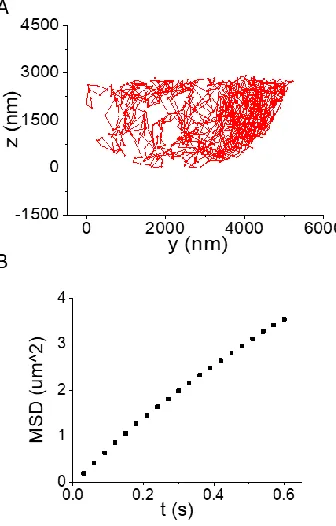
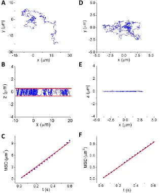
Figure 2.1. 3D trajectory of a 100 nm nanoparticle diffusing on a 2600 nm oil droplet surface. ... 45
Figure 2.2. 3D trajectory of a 100 nm nanoparticle diffusing on a 690 nm oil droplet surface. ... 47
Figure 2.3. Simulated trajectories of particle diffusing on droplet surface. ... 51
Figure 2.4. Recovered diffusion coefficient using linearized Castro-Villarreal Equation ... 53
Figure 2.5. Recovering diffusion coefficient using Castro-Villarreal Equation truncated to different orders of polynomials. ... 57
xi
Figure 2.7. Schematics of particle diffusion at oil-water interface. ... 61
Figure 3.1. Point spread functions at different extent of astigmatism and schematic of experimental design ... 76
Figure 3.2. Localization of 100 nm polystyrene particles’ z position with 1 µm PSF. ... 78
Figure 3.3. Correlation coefficients at different z positions ... 79
Figure 3.4. Different axial localization precisions of 100 nm polystyrene particle using different PSFs at high and low photon flux situations. ... 82
Figure 3.5. 100 nm particle diffusing in a 1 µm thick channel ... 84
Figure 3.6. 100 nm nanoparticle diffuses inside 5 µm diameter water droplet ... 85
Figure 3.7. 3D domain structure on supported lipid bilayer with 5% GM1 ... 86
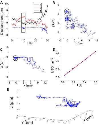
Figure 4.1. 100 nm polystyrene particle diffusing in a channel and on SLB membrane surface. ... 97
Figure 4.2. 100 nm particle diffusing on solid supported lipid bilayer at pH 7.4. ... 100
Figure 4.3. Two representative examples of particle adsorption/desorption on lipid bilayer surface. ... 102
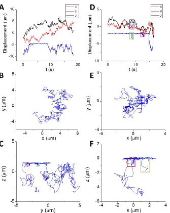
Figure 4.4. A representative trajectory of particle diffusion on lipid bilayer surface at pH 10.0. ... 104
Figure 4.5. Another representative trajectory showing the 3D structure of the domains at pH 10.0. ... 106
Figure 4.6. Lipid domains and their effects on particle diffusion. ... 108
Figure 5.1. Schematic of a 3-layer convolution neural network structure. ... 124
Figure 5.2. Probability distribution of images and super localization in the z-direction. ... 125
Figure 5.3. S/N at different integration times for the same 200 nm fluorescent particle. ... 128
xii
Figure 5.5. Performance of DNN and CC for low S/N (S/N = 1) data. ... 133
Figure 5.6. Performance of DNN and CC for low S/N data (S/N =1) with artificial noise .... 134
Figure 5.7. Performance of DNN and CC methods for experimental data collected at 50 s ... 137
Figure S5.1. Typical images from 29 sets of PSFs, respectively. ... 141
Figure S5.2. Example images with different S/N and the impact of S/N on correlation coefficient. ... 142
Figure S5.3. Recovered 3D trajectory of a 100 nm particle diffusion on an oil droplet surface using DNN method. ... 143
Figure S5.4. Performance of DNN and CC for low S/N data (S/N =1) with experimental noise ... 144
Figure S5.5. Performance of DNN and CC methods for experimental data... 145
Figure S5.6. Accuracy and precision tests of localization of 40 nm polystyrene particles. ... 146
Figure 6.1. Training and testing using stepping data. ... 159
Figure 6.2. Testing data with a constant background. ... 162
Figure 6.3. Test data with a constant background ... 163
Figure 6.4. Two particles completely over each other but with different axial positions. ... 165
Figure 6.5. Two particles with different extent of lateral overlap along the x-axis ... 167
Figure 6.6. Experimental data of 100 nm particles diffusing on an oil droplet and in the solution. ... 170
Figure S6.1. Schematic of CNNs. ... 173
Figure S6.2. Optimizing the structure of CNNs ... 174
xiii LIST OF PUBLICATIONS
1. Zhao, L.; Zhong, Y.; Wei, Y.; Ortiz, N.; Chen, F.; Wang, G., Microscopic movement of slow-diffusing nanoparticles in cylindrical nanopores studied with three-dimensional tracking. Anal. Chem. 2016, 88 (10), 5122-5130.
2. Zhong, Y.; Zhao, L.; Tyrlik, P. M.; Wang, G., Investigating Diffusing on Highly Curved Water–Oil Interface Using Three-Dimensional Single Particle Tracking. J.Phys.Chem.C. 2017, 121 (14), 8023-8032.
3. Zhong, Y.; Wang, G., Three-Dimensional Heterogeneous Structure Formation on a Supported Lipid Bilayer Disclosed by Single-Particle Tracking. Langmuir 2018, 34 (39), 11857-11865. 4. Zhong, Y.; Li, C.; Zhou, H.; Wang, G., Developing Noise-Resistant Three-Dimensional Single
Particle Tracking Using Deep Neural Networks. Anal. Chem. 2018, 90 (18), 10748-10757. 5. Zhong, Y. and Wang, G.*, Overcome Interfering Background for Multiple Particle Tracking
in Three-Dimensional Space using Deep Neural Networks. Manuscript in Preparation. 6. Zhong, Y. and Wang, G.*, 3D Single Particle Tracking in Analytical Chemistry. Annu. Rev.
Anal. Chem. 2019, Invited Review.
1 Chapter 1. Background and Significance
1.1. Overview
Conventional two-dimension (2D) single particle tracking (SPT) has been a powerful tool for various biological and chemical studies. However, most of the real-world samples are three dimensional (3D) in nature. In this dissertation, we are developing robust 3D SPT techniques with high resolution that can be used in complicated chemical and biological environments. The effect of the engineered point spread functions (PSFs) on localization accuracy and precision has been systematically studied (Chapter 3). With the current astigmatism-based SPT technique, we successfully studied nanoparticle diffusing on the highly curved oil-water interface (Chapter 2) and on the planar supported lipid bilayers (Chapter 4). At the end, we are incorporating deep learning neural networks (DNNs) in the 3D data analysis to overcome practical problems including high noise (Chapter 5) and high background (Chapter 6) in complicated chemical and biological systems.
1.2. What Can Single Particle Tracking Do?
2 coexistence and domain formation in lipid bilayers that play essential roles in cell functions.3 In addition, SPT has been used to probe a variety cellular activities such as receptor activation, signaling processes, dynamics of endocytosis and exocytosis, and the mechanisms of entry, trafficking, and egress of various viruses, etc. Its applications in biological studies have been well reviewed in the literature.4-10
3 1.3. Current Three-Dimension Single Particle Tracking Techniques
Due to the indispensable functions, single particle tracking techniques have been studied for over decades and there are various types of techniques based on different mechanisms being developed. Most of the single particle tracking techniques are based on fluorescence microscopy due to their extraordinary sensitivity and ability of real time imaging. Unlike imaging techniques such as X-ray, electron or atomic force microscopy, the fluorescence microscopy has low risk of interrupting the samples since it has relative lower energy and no need to touch the sample directly, which makes it a perfect tool study biological problem at molecular level. Conventional fluorescence microscopies are limited by the poor resolutions caused by the diffraction limits (~250 nm), which means two fluorophores can’t be distinguished when their distance is smaller than the diffraction limit.27 Recently, great efforts have being made to overcome the diffract limits through multiple approaches, including Structured Illumination Microscopy (SIM)28, Stimulated Emission Depletion (STED) Microscopy29 and Stochastic Optical Reconstruction Microscopy (STORM)30, and they have successfully pushed the resolution of the optical microscopy to 1/10of the diffraction limits for single fluorophore. These groups of techniques are so-called “Super”-Resolution Optical Microscopy, which refers to a resolution below the diffraction limit.
4 three-dimensional images for two main reasons: (1) the symmetric distributed PSF about the focal plane causes difficulties to distinguish spots with the same distance above and below the focal plane and (2) a certain depth between the particle and the focal plane is needed to obtain the out-of-focus pattern, which means that the particle’s position is difficult to obtain when it is on or near the focal plane.27
Recently, there have been great efforts in developing 3D SPT techniques. The core concept of these improvements is to make use of the different patterns and/or signal intensities from the particles localized in different axial positions to obtain the information from the third dimension. Depending on the working principle, current 3D localization and tracking techniques can be classified in three categories: multi-plane collection, distorting image patterns and interface-based techniques31-35:
5 noise, which leads to short trajectories, low localization precision (50~100 nm), and expensive and complicated instrumentation, etc.
(2) The axial information can also be obtained through distorting image patterns (point spread functions) in wide field mode. Rather than scanning the sample in the object side, this method is equivalent to scanning the detector in the image space, which yields the same axial information of the sample. To minimize the number of the exposures to be 1, images in different imaging planes are exposed to the same detector chip at once. These designs include chromatic astigmatism-based imaging,32-33 and double-helix PSF39, etc.
(3) Axial tracking can also be achieved using interface-based techniques such as total internal reflection fluorescence (TIRF) microscopy.31, 40-42 However, interface-based techniques highly rely on an interface and usually have a very short working range (~200 nm) compared to other methods, which limits their applications.
1.3.1. Multi-Plane Imaging
This group of methods contain many variations and they are mainly depending on imaging the object at several planes, which can obtain the particles’ axial position information. This group of techniques includes bifocal/multifocal imaging,43-49 parallex50-51 and confocal imaging.38, 52-53 1.3.1.1. Bifocal/multifocal Plane Microscopy
6 interest for in particle tracking. Bifocal imaging methods43, which could provide two images (focused and defocused) of the same particle simultaneously, could get 3D positions.
The central part of these methods is the introduction of a beam splitter, which can divide the emission light beam in front of the camera into two beams with adjustable intensity ratio and different direction. Then one beam is reflected by a mirror (with a longer path) while the other one transmitted directly through the beam splitter (with a shorter path) before they directed toward the CCD. Due to the different optical paths, there will be two patterns formed for the same particle (both focused and defocused, shown in Figure 1.2.b) due to a relative focal plan shift between the two beams. As mentioned before, particles with different axial positions in the sample will have a different defocused patterns radius so the z information from the defocused image. However, the defocused images are not accurate enough for characterizing the x-y position, so it is needed to split the beam into two part to form a focused pattern to obtain the accurate axial position.
7 A problem with bifocal imaging is that a standard microscope must be changed in a significant way by replacing its standard emission optics with a custom setup due to the need for adjustment of lens to focus the image on the detector. What’s more, the weak signal intensity also limits the application of bifocal imaging.
The main advantages of bifocal/multifocal imaging techniques are the high position accuracy (up to 10 nm), fast imaging rate (up to 150 nm/ms for single particle tracking and 12 frames/s for intracellular imaging) and the ability of continuous detection. Bifocal/multifocal imaging could be applied in many kinds of microscopy, such as wide-field microscope, STORM, PALM, etc. Manuel F Juette and coworkers54 have combined the bifocal techniques with FPALM and showed great performance for the detection of thick biological samples with a 30 nm lateral accuracy and 75 nm axial accuracy over a depth of several micrometers without compromising speed or sensitivity.
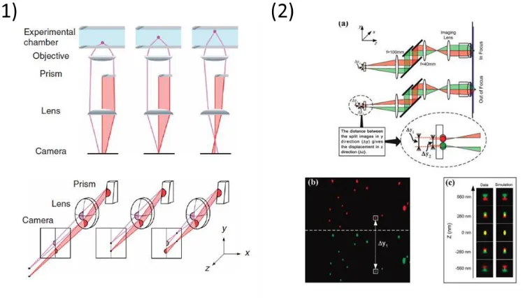
1.3.1.2. Parallax
8 around the sample plane into x-directed movement, perpendicular to both the prism axis (y axis) and the optical axis (z axis), at the equivalent sample plane.
In comparison, Yujie Sun and coworkers51 used a pair of closely spaced, nearly parallel mirrors (Figure 2.2) that achieved the same function as prism and termed parallax. When a small object is in focus, its beam flux is collimated by the lens. With the effect of these mirrors, the beam flux is split into two paths that form two focused spot images on the upper and lower halves of the camera chip separated by a distance Δy1. When the object goes out of focus, its beam flux is no longer collimated and the split images, defocused patterns instead of focused spots, formed on the camera are closer to or further away from each other with a separation of Δy2. The difference between Δy1 and Δy2 provides the signal for measuring displacement of the object in the z direction (Δ z). When the distance between the particle and the objective changes, there are different patterns shown on the camera. By comparing these patterns with a prepared calibration database, we could get the accurate position information along the z axis.
9 This method is similar with the bifocal imaging technique since they both utilize the defocused pattern to localize the z position and focused pattern to localize the x-y position. The difference, also the main advantage, from a bifocal or astigmatism imaging is that the determination of the z position didn’t rely on the orientation or the shape of the defocused patterns. Instead, the displacement in the z direction is linearly related to the relative distance in the y direction between each pair of spots in the split images, the centers of which can be precisely measured. In contrast with multifocal or astigmatism imaging, this insensitivity to the PSF shape makes this method not subject to the aberrations and polarization and make it more accurate since the center of the patterns could be determined much more accurate than a shape parameter. Another advantage of this method is that they don’t need complicated and expensive setups and involves only simple modifications to achieve 3D tracking just by using commercially available optical devices, which will significantly extend this technique to a wide range of applications. They could also provide images with high spatial resolution and the temporal resolution is only limited by the CCD frame rate/signal strength. The expected combination of new super resolution techniques such as STORM could make further improvement for the spatial resolution.
1.3.1.3.Confocal Imaging
10 used confocal microscopy operating in fluorescence mode to study the structure and the dynamics of colloidal particles. They could get the 3-dimention position of several thousand particles at once with a precision of 50 nm in all the three directions.
Compared with methods with fixed focal plane such as astigmatism and multifocal, which are generally limited in their z-tracking range of approximately ±1μm from the focal plane due to the shallow depth of field of the objectives, the confocal microscope could reach a wider z range as tens of micrometers, just depending on the movement of the stage and the working distance of the objective. The limitations of confocal microscope for 3D tracking are also obvious. It usually takes seconds to minutes to obtain one 3D images at once, which limited the application of confocal microscope due to the great losses of details of the movement of high-speed particles in big volume.
11 Recently, a group led by Werner52 revised the confocal method successfully (Figure 3) to accomplish 3D single particle tracking that kept the advantages of confocal microscopy with large z-range and avoided the limitation of the low temporal resolution. Four confocal fiber optics serve as spatial filters to examine four nearly diffraction limited spots in the sample simultaneously. Because of the spacing and arrangement of the fibers, these four spots form a 3D tetrahedron in the sample space. While tracking, active feedback of a XYZ piezo stage is used to keep counts on all four detectors equally and as large as possible. A small fraction (∼8%) of the emission light from the molecule being tracked is sent to an EM-CCD camera, which enables contextual information for the position of the molecule in the cell during 3D tracking. The main part of this method is the use of four overlapping confocal volume elements and a fast XYZ positioner for real-time feedback depending on the particle’s position in every 5 ms. Tracking is achieved by a simple feedback algorithm in which, for each time slice, pulses from each detector are counted and analyzed to estimate the likely position of the current target. The sample stage is then moved to bring the target closer to the center of the laser focus. This process is repeated every time slice until the signal drops to the level of the background noise, at which time the particle is considered lost. The instrument then returns the stage to the center position, where it is stationary until another target enters the detection volume.
1.3.2. Distorting Image Patterns
12 pathway and for a typical microscope, the point spread function is called Airy disk which, mathematically, is related to the first-order Bessel function of the first kind. By manipulating the optical pathway, the point spread functions can be distorted from Airy disk into various 3D shapes, in which the complicated defocused image patterns are a function of the particle’s axial positions. The distorted point spread functions (PSFs) make 3D single particle localization possible. These set of techniques are similar to defocused imaging methods since they both utilized the defocused image patterns to localize the particles in the axial direction. The difference here is the patterns in these sets of methods have orientations and polarizations towards different directions instead of a set of circle patterns in defocused imaging. This group of methods mainly contain two types: astigmatism imaging 32-33 and double-helix PSF based imaging.39, 55-57
1.3.2.1.Astigmatism Imaging
13 Figure 1.4. Schematic of astigmatism based single particle tracking. (1) Schematic of a typical astigmatism setup. (2) Calibration curve of wx and wy as a function of z. Reprinted with permission from ref 33. Copyright 2008 by the American Association for the Advancement of Science.
To determine particles’ z positions from the astigmatism imaging, a set of pre-collected calibration data sets containing particle’s different point spread function (PSF) at different axial positions are usually needed. There are mainly two group of data analysis methods in astigmatism-based single particle tracking: fitting and image classification algorithm. Fitting can be used to analyze simple point spread functions, such as elliptical shape.33 2D Gaussian function is applied to fit the elliptical point spread function (PSF) to obtain the x, y peak center as well as the peak width wx and wy. The x, y peak center represents the lateral position while the peak width contains the information of axial position (calibration curve shown in Figure 1.4 (2)). The problem of the fitting method is when the point spread function (PSF) become complicated and noisy, it is very challenging to obtain the mathematic model of patterns to fit. In this case, image classification method, such as correlation coefficient method and machine learning, can provide much better localization accuracy. We will discuss this part in detail in the later part this chapter.
14 imaging rate (only limited by the frame rate of CCD camera/signal strength) and simple setups (minimal optimization on a commercial widefield microscopy).
1.3.2.2.Double-Helix PSF
Moerner and coworkers55 demonstrated a method to super-localize single particle z position with a widefield fluorescence microscope exhibiting a double-helix point spread function (DH-PSF). This method, showing a ∼10 nm localization capability along x, y, and z even with weak emitters, was used to track single quantum dots in aqueous solution as the demonstration. The DH-PSF is generated by inserting an all-optical 4f image processing section (Figure 1.5A) to the detection path of a conventional inverted microscope. The addition of 4f setup is to convolve the standard spherical point spread (PSF) function with the DH-PSF. Such performed convolution is Fourier transferred by another lens and restore a real space image on detector (Figure 1C). After revising the standard upright microscope, the point spread functions on the detector of the point light source become two lobes with unique orientations, which is a function of the object’s z positions. Therefore, it can be used to track particles in 3D space.
15 Figure 1.5. Schematic and experimental characterization of the DH-PSF imaging system. (A) Schematic of the 4f setup that is attached to the detection path of a standard inverted microscope. (B) Top panels are xy and yx cross section of a DH-PSF while the bottom panels are from the standard PSF from a conventional microscope. (C) and (D) restored real space image pattern on detector and its fitting output. Reprinted with permission from ref 55. Copyright 2009 American Chemical Society.
1.3.3. Intensity-Based Techniques
16 1.3.3.1.Fluorescence Lifetime Imaging Microscopy (FLIM)
FLIM and FLIC are methods that suitable for the areas close to a surface. Tracking the point objects achieved in an indirect way compared to conventional microscopy. Rather than imaging the targets directly on the camera, FLIM is a novel method for 3D tracking since they utilized the lifetime of the fluorescing molecules labelled near a metal surface. The molecules have different lifetimes when they have different distances away from the metal or silicone surface, which can be utilized to localize the molecules in the axial direction.
Figure 1.6. Schematic of FLIM experimental setup. Fluorescently labeled microtubules are elevated to different z positions with the help of spacer above a 15 nm thick gold membrane surface in a microscope flow cell. At different z positions away from the surface, the fluorescence lifetime collected by the FLIM system is different (shown in upper right figure). Reprinted with permission from ref 42. Copyright 2010 American Chemical Society.
17 flurophore in aqueous condition. This limit is ~100 nm, which means this method only has a z working range of 100 nm near the surface. This method, coupled with FLIC shown below, could only be used in a specific area near either a metal or a silicon surface, which largely limited its applications despite of its high accuracy. However, they provide new perspectives for the SPT techniques, which is significantly different from the regular microscopy.
Figure 1.7. Principle of fluorescence interference contrast microscopy (FLIC). Reprinted with permission from ref 31. Copyright 2008 Nature Publishing Group.
1.3.3.2.Fluorescence-Interference Contrast Microscopy (FLIC)
18 rotation of the microtubules. As mentioned above, this technique is also limited to the silicon surface and the working range is only 100 nm.
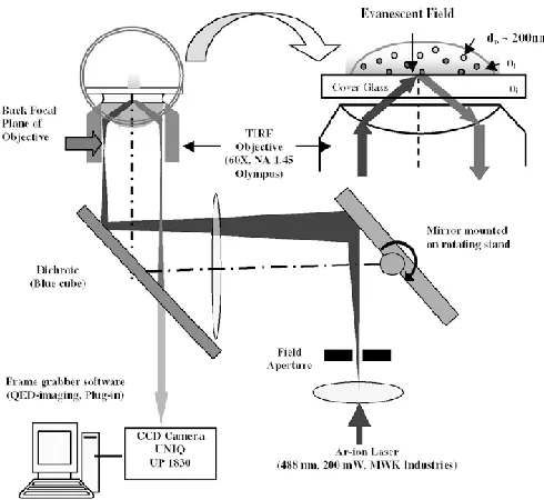
Figure 1.8. Schematic of 3D Total Internal Reflection Fluorescence Microscopy. Reprinted with permission from ref 41. Copyright 2004 Springer-Verlag.
1.3.3.3.Total Internal Reflection Fluorescence Microscopy (TIRFM)
Unlike the first two method, total internal reflection fluorescence microscopy (TIRFM) is a much more commonly used technique especially in studying cellular organization and dynamic processes near the cell culture and glass substrate interface. Not like common wide field fluorescence microscopy, the light source in TIRFM is the evanescent field (EF), which is produced when an incident light beam traveling from a high refractive index medium to a low one with an incident angle greater than the critical angle. The evanescent field intensity (I) decays exponentially when the distance from the surface increases and follows such equation:
/ ( ) 0
( )
z dI z
=
I e
− 19 resolving the probe’s axial distances away from the interface. The exact evanescent field at different z positions can be calibrated by attaching the florescent particles to AFM arms and changing the axial positions of particles. The working range of TIRFM is usually ~150 nm and the effective distance is affected by various factors including polarization of excitation light, orientation of dipoles, the unevenness of the illumination light, and so on. Figure 1.7. shows the schematic of a 3D TIRFM to study the near-wall hindered Brownian motion of polystyrene particles.
The main shortcoming of TIRFM is the short z working distance (~100 nm) and the need of a glass surface to generate evanescent field. However, due to the shallow illumination depth of evanescent field, the image background is much lower than epi-fluorescence microscopy due to the missing of fluorescence background from out-of-focal region of the samples, which makes is an ideal tool to study single molecules. Xiaowei Zhuang’s group33 successfully implement 3D STORM on TIRFM and achieved 50 nm resolution along the axial direction.
1.3.4. Experimental Setup of 3D Single Particle Tracking
20 20~30 nanometers in the axial dimension could be achieved for ~100 nm fluorescent particles and the temporal resolution can be up to 8 ms/frame.59
Figure 1.9. Schematic of astigmatism-based 3D single particle tracking. (1). Instrument setup of imaging system. (2) Point spread functions at different extent of astigmatism. (A) 1 um focal plane gap. The distance between two frames is 200 nm. (2B) 3 µm focal plane gap. The distance between two frames is 1000 nm. (2C) 10 um focal plane gap. The distance between two frames is 200 nm.
21 precision due to a decreased signal to noise ratio. So, it is a compromise and we need to pick the proper PSFs for specific studies. For instance, for studies about particles diffusing on planar lipid bilayers and the flurophores are single molecules or small particle with low fluorescence intensity, a small PSF is preferred due to the limited axial movement and low intensity. On other hand, when the probes moving in a larger 3D space, such as porous materials and cellular systems, 5 µm-sized PSFs become necessary to track the particle continuously.
1.4. Data Analysis Methods in Single Particle Tracking
Compared to other multifocal plane imaging, the advantage of astigmatism-based imaging is that it collects images from all different imaging planes (rather than 2, for example, the two-color bifocal plane imaging), yielding the most amount of the axial information. However, all images at different imaging planes are superimposed on the same camera chip, resulting in a very complicated point spread function (PSF), where PSF refers to the light intensity distribution in the imaging side for a point object. Therefore, the data analysis becomes challenging for these complicated image patterns. For the small PSFs (like the ellipses), 2D Gaussian function can be utilized to predict the image pattern and the axial position obtained by estimating the aspect ratio of the ellipses. For the large diamond shape PSFs (Figure 1.9.2), it is nearly impossible to fit such complicated PSFs with explicit functions. Developing other data analysis method is necessary.
22 neural networks, which utilize the calibration image sets as the training set to train either mathematic models or neural networks to classify experimental images.
Correlation coefficient method is a simplified linear machine learning method, which presumes that the calibration image sets are well trained model and using this model to evaluate the experimental data by calculating their correlation coefficients. This is partly true only when experimental data and calibration data are collected under same experimental condition and have high image quality including high S/N ratio and low interfering background. With the restriction of similar image qualities, correlation coefficient method does show decent localization accuracy and precision. However, in more common and realistic conditions, when noise and interference background can’t be avoided, correlation coefficient method shows its limitations since the assumption that calibration sets represent the real model is no longer valid.
Therefore, in order to obtain models closer to the authentic model, machine learning algorithms are needed to abstract the information from calibration sets collected under various experimental conditions. Such trained models show much high resistance to noise and interfering background when comparing test data to the calibration model sets. For image classification, traditional machine learning methods are still ideal since the statistical models, at most time, are not sufficient for image data which contain numerous features in the presence of interfering background.
23 methods including correlation coefficient, conventional machine learning, and deep neural networks are introduced.
1.4.1. Correlation Coefficient Method
In conventional optical microscopy, the PSF of a point object can be expressed using the Bessel function. In the focal plane, the image pattern is an Airy disk, which can be further approximated as a two-dimensional (2D) Gaussian distribution function. The object’s 2D positions can be recovered with high precision (usually sub-pixel length scale) using non-linear least squares (NLLS) fittings. However, in our astigmatism-based 3D tracking, the complicated image patterns make data analysis challenging. Thus, how to extract the axial positions from the complicated image patterns is the key in 3D tracking as well as 3D super resolution optical imaging. Due to the optical aberrations of individual imaging systems, it is difficult to predict the exact theoretical imaging patterns. Currently, the most frequently used method is manual calibration, which includes the collection of an empirical calibration set. For simple image patterns, the most significant feature can still be empirically extracted, which serves as a guide for the prediction of the sample spatial informatiaon.3, 60-61 For complicated imaging patterns, more sophisticated pattern recognition methods are required. A universally applicable and arguably the most reliable pattern recognition method currently is the Pearson Correlation Coefficient method (CC). In this method, the sample is compared pixel-to-pixel with each image in the calibration set. The similarity is determined based on the correlation coefficient p, which is defined as:
= − − − = m i sample sample sample model modelmodel i I avg I i I avg
24 calibrated z-values is sparsely distributed over the whole z-range), a weighing or fitting procedure is usually used to obtain sub-frame resolution.
Figure 1.10. Example images with different S/N and the impact of S/N on correlation coefficient. (A) The same image (S/N 100) superimposed with artificial Gaussian noise so their final S/N ratios are 1, 5, 10, and 40, respectively. Scalebar: 5 m. (B) The correlation coefficient between the original image (S/N ~40) with the image superimposed with different levels of artificial Gaussian noise.
25 problem in high sensitivity optical imaging: the total number of the photons is limited from a single molecule/nanoparticle within a certain frame time. Thus, developing an algorithm that is resistant to noise is important to both the time resolution and spatial resolution (i.e., localization accuracy and precision) for 3D single particle tracking.
1.4.2. Statistical Machine Learning
Statistical machine learning includes methods that builds statistical models based on known data and uses such models to predict and analyze unknown data.62-64 Machine learning contains supervised learning, unsupervised learning, and reinforcement learning. In this section, we mainly discuss supervised learning in which all the data used for training are well labeled and classified. A typical procedure of statistical machine learning includes: (1) obtain limited amount of training data with correct labels. (2) Select a set of possible training model. (3) Use learning algorithm to train and evaluate all the possible models and select the one with the lowest expected loss. (4) Predict the new data with trained model. Generally, for input data X and output classification result Y, the goal of statistical learning is to train models with the decision function
(X)
Y = f , or conditional probability distributionP Y X( | ), which are equivalent. A loss function L(yi, f(xi)) , which is related to the true value yi and the predicted value f(xi), is used to measure the extent of the erroneous prediction. In the training, the loss (either empirical or structural loss) is minimized to determine the model (decision function), which will be used to predict data in the sample set.
Decision-26 Making Tree, Logistic Regression/ Maximum Entropy Model, Perceptron). The most significant difference between generative and discriminative approaches is the former one will generate the decision function (or, the joint probability distribution) from the constraints (i.e., data in the training set (xi, yi)), while discriminative algorithm only explores and optimizes the decision function in a given hypothesis space for models. In supervised learning, both generative and discriminative approaches have their own merits and demerits and are suitable for different types of learning problems.
1.4.2.1.Generative Approach
Generative approach will first learn relation between input X and output Y, which is the joint probability distribution P X Y( , ) from the training set, and then calculate the conditional probability distribution P Y X( | ):
( , ) ( | )
( ) P X Y P Y X
P X
= (2)
The main advantages for generative approaches over discriminative approaches are: (1) they can express the complex relationships between data and prediction variables. (2) They have quicker convergence speed, which means generative approaches can learn the models faster especially with large training data set. In this subsection, we will discuss a representative generative approach: Naïve Bayes approach.63, 65-66
27 Y with maximum a posterior probability (MAP) calculated using Bayes theorem. Naïve Bayes classifier is easy to implement and has high training and predicting efficiency.
In our case, the training data are n images with N pixels (input N
X R ) labeled with K
different z positions (output K
YR ). The training data set:
T
=
{( , ), ( ,
x y
1 1x y
2 2), , ( ,
x y
n n)}
follows joint probability distribution P X Y( , ) . Essentially, the naive Bayes is a conditional probability model given that the features represented by a vector(
) (
|
)
(
) (
|
)
(
|
)
(
)
(
|
) (
)
k k k k
k
k k
k
P Y
z P X
x Y
z
P Y
z P X
x Y
z
P Y
z
X
x
P X
x
P X
x Y
z P Y
z
=
=
=
=
=
=
=
=
=
=
=
=
=
=
prior likelihood
posterior
evidence
=
(4)To learn the P X Y( , ), we first need to calculate the prior probability with maximum likelihood estimation (MLE):
1
(
)
(
)
,
1, 2,
,
n
i k i
k
I y
z
P Y
z
k
K
n
=
=
=
=
=
(5)Then, the conditional probability distribution (likelihood) according to naïve independence assumption:
(1) (1) ( ) ( )
( ) ( ) 1
(
|
)
(
,
,
|
)
(
|
)
N N k k N i i k iP X
x Y
z
P X
x
X
x
Y
z
P X
x
Y
z
=
=
=
=
=
=
=
=
=
=
(6)28
( ) ( )
( ) ( )
( ) ( | )
( | ) , 1, 2, ,
( ) ( | )
i i
k i k
k i i
k k
k i
P Y z P X x Y z
P Y z X x k K
P Y z P X x Y z
= = = = = = = = = =
(7) For all z position labels of Y (z
1, ,
z
K), the final output z position of input image x is the z value that give the maximum a posterior probability (MAP) (Equation 7):( ) ( )
( )
arg max (
)
(
|
)
k
i i
k i k
z
y
=
f x
=
P Y
=
z
P X
=
x
Y
=
z
(8)When the posterior probability reaches the maximum value, the expected loss of trained model is the lowest, which means the model is the optimized in Naïve Bayes approaches. In this subsection, we used maximum likelihood estimation (MLE) to estimate the prior probabilities and conditional probabilities. Bayesian estimation can also be used and sometimes, it shows better results than MLE since the MLE might evaluate the probability as 0 by mistake.
In image classification, the features (pixel intensities) can be viewed as a continuous variable. A typical assumption needs to be taken that the continuous values are distributed according to a Gaussian distribution. For example, for each class, the ith pixel has a mean of and a standard deviation of σ (which can be calculated from the training set). Suppose we collected an observation value probability distribution of given a class zK, P(X = can be estimated as:
2
2 2
1
(
)
(
|
)
exp(
)
2
2
k
P X
Y
z
−
=
=
=
−
(9)while the rest part of the derivation keeps the same. 1.4.2.2.Discriminative Approach
29
( | )
P Y X , from the training set, and use it to predict the unknown test data. Because for
discriminative approach, the prediction is directly based on the training process, so the learning accuracy is higher than generative approach. What’s more, it can greatly simplify the learning problem by abstracting input features and adding self-defined new features. In this subsection, we will mainly discuss commonly used discriminative classifier: logistic regression model.65, 67-71
Figure 1.11. Density function (1) and distribution function (2) of logistic distribution.
Logistic regression/Maximum entropy model (MEM). Logistic regression and maximum entropy methods are practical identical because exponential model for multinomial logistic regression, when trained according to the maximum likelihood criterion, also finds the maximum entropy distribution subject to the constraints from the feature function (training set).
In logistic regression, it assumes a logit linear model. Taking binomial logistic regression model as an example, the distribution function (2) and density function (1) of logistic distribution are shown in Figure 1.11. The distribution function of logistic distribution is sigmoid curve in which the probability increases faster near the center and slower at the two ends. To simplify the discussion, binominal logistic regression model is introduced, and it will be expanded to multi-nominal model. Assuming that we have two sets of training set with z value either 0 or 1 and
( 1| )
p=P z= x . The odds for particle having z position as 1 is defined as
1
p
p
30 ratio of probability of z=1 and z = 0. For logistic regression model, the main assumption is that the log odds (or logit function) is linear function of input x:
(
1| )
log
log
1
1
(
1| )
p
P z
x
w x b
p
P z
x
=
=
= +
−
−
=
(10)If we solve this equation, we can get the conditional probability distribution:
exp(
)
(
1| )
( )
1 exp(
)
w x b
P z
x
f x
w x b
+
=
=
=
+
+
(11)1
(
0 | )
1
( )
1 exp(
)
P z
x
f x
w x b
=
=
= −
+
+
(12)The classification algorithm is for any given input image x, calculate the two probabilities using Equations (11) and (12) and the final output z value has larger probability. The next issue is to train and estimate the weights w and b with maximum likelihood estimation (MLE). The likelihood function of this distribution is:
1
1
[ ( )] [1
i( )]
iN
z z
i i
i
f x
f x
−=
−
(13)The logit likelihood function is:
1
1
1
( )
[ log ( ) (1
) log(1
( ))
( )
[ log
log(1
( ))]
1
( )
[ (
) log(1 exp(
)]
N
i i i i
i N i i i i i N
i i i
i
L w
z
f x
z
f x
f x
z
f x
f x
z w x
b
w x
b
= = =
=
+ −
−
=
+
−
−
=
+ −
+
+
(14)31 expand to multi-nominal model. For K different z values in the training set, the conditional probabilities for all K different z values are:
1
1
exp(
)
(
| )
,
1, 2,
,
1
1
exp(
)
i K
i k
w x
P z
i x
i
K
w x
−
=
=
=
=
−
+
(15)1
1
1
(
| )
1
exp(
)
K
i k
P z
K x
w x
−
=
=
=
+
(16)1.4.3. Deep Learning Neural Networks
Traditional machine learning algorithms performs poorly when applied to analyze image data for several reasons: first, the image data are much more complicated than numerical data and the machine learning models are usually too simple to model image data; second, machine learning algorithm can’t be used to model large dimension image data due to the convergence issue. For example, for an image data set containing 1000 images and each image is 1000 * 1000 pixel size, if we train such data with the simplest logistic regression model, the number of parameters need to train is 1000 * 1000000. It becomes practically impossible to fit such a large number of parameters, and it will suffer from overfitting problem.
32 give more global features because all the shallow layers contribute to the deep layers. Informally, for the functions one can compute with “small” deep neural network, the shallower networks require exponentially more parameters to achieve similar performance. Two of the most widely used deep neural networks nowadays are convolutional neural network (CNNs) for image recognition and recurrent neural network (RNNs) for voice detection and natural language processing. Among various DNN architectures, we will focus on convolutional neural networks (CNNs) in this project given their superior image recognition performance in various image recognition competitions.72-73
Figure 1.11. Schematic of a convolutional neural network. (A) shows how an input image is analyzed through a convolution neural network and outputs its categories. (B) typical structure of 1-layer convolution neural network.
33 more abstract low-resolution feature maps. These are realized by two alternating types of layers: convolutional and pooling layers. The last few layers are fully-connected classifiers that combine all features together to produce the abstracted classification results.
A convolutional layer extracts various features such as oriented edges, corners and crossings from input feature maps via convolutional filters, and then combines them into the more abstract output feature maps. The features in each feature map are a 3D volume data with three dimensions: width, height and depth. With the large image data set and the massive computation power of parallel computers such as Graphics Processing Units (GPUs), state-of-the-art CNN frameworks choose to process multiple images in a batch.74 Thus, the input to a convolutional layer includes feature maps from multiple images and is organized as a four-dimensional (4D) array. The computation in the convolution stage is shown in Equation 17, where Ni is the batch size, Ci is the depth or number of input feature maps, Hi and Wi are the height and width of feature map, Fhand Fw represent the size of the convolution filter kernel, and Co is the output feature maps or the number of filters.
0 0 0
[ ][ ][ ][ ] H W [ ][ ][ ][ ] [ ][ ][ ][ ]
i w
C F F
o i i C h f i i i h i w o i h w
Out Ni C H W =
= = = in N C H + f W + f filter C C f f34 increases the translation invariance of the network, which means the position of object in the images won’t affect its classification.
A classifier (Softmax) layer is the final layer of a CNN for classification, which computes the possibility distribution over different labels. Before the softmax layer, there usually exist full-connected layers, which flatten the 4D feature maps into a 2D matrix. A standard matrix multiplication is used to implement a fully-connected layer.74 The output is the probabilities that a sample image belonging to one of the class (i.e. z values in our case), respectively. In the case of complete calibration sets, the probabilities will be normalized. Specifically, the output will be fed into the softmax layer. The softmax layer will first find the maximal possibility over each batched image. Then, each probability is shifted by the maximum. Next, an exponential operation is performed on each probability. Last, all probabilities are normalized.
35 1.5. References
1. Kural, C.; Kim, H.; Syed, S.; Goshima, G.; Gelfand, V. I.; Selvin, P. R., Kinesin and dynein move a peroxisome in vivo: a tug-of-war or coordinated movement? Science 2005, 308 (5727), 1469-1472.
2. Kural, C.; Serpinskaya, A. S.; Chou, Y.-H.; Goldman, R. D.; Gelfand, V. I.; Selvin, P. R., Tracking melanosomes inside a cell to study molecular motors and their interaction. Proc. Natl. Acad. Sci. U.S.A. 2007,104 (13), 5378-5382.
3. Levi, V.; Gratton, E., Exploring dynamics in living cells by tracking single particles. Cell biochemistry and biophysics 2007,48 (1), 1-15.
4. Dix, J. A.; Verkman, A. S., Crowding effects on diffusion in solutions and cells. In Annual Review of Biophysics, 2008; Vol. 37, pp 247-263.
5. Brandenburg, B.; Zhuang, X. W., Virus trafficking - learning from single-virus tracking. Nature Reviews Microbiology 2007,5 (3), 197-208.
6. Laude, A. J.; Prior, I. A., Plasma membrane microdomains: organization, function and trafficking (Review). Molecular Membrane Biology 2004,21 (3), 193-205.
7. Kusumi, A.; Tsunoyama, T. A.; Hirosawa, K. M.; Kasai, R. S.; Fujiwara, T. K., Tracking single molecules at work in living cells. Nature Chemical Biology 2014,10 (7), 524-532. 8. Saxton, M. J.; Jacobson, K., Single-particle tracking: Applications to membrane dynamics.
Annu. Rev. Biophys. Biomol. Struct. 1997,26, 373-399.
9. Shen, H.; Tauzin, L. J.; Baiyasi, R.; Wang, W. X.; Moringo, N.; Shuang, B.; Landes, C. F., Single Particle Tracking: From Theory to Biophysical Applications. Chem. Rev. 2017,117 (11), 7331-7376.
10. von Diezmann, A.; Shechtman, Y.; Moerner, W. E., Three-Dimensional Localization of Single Molecules for Super Resolution Imaging and Single-Particle Tracking. Chem. Rev. 2017, 117 (11), 7244-7275.
11. Bevan, M. A.; Prieve, D. C., Direct measurement of retarded van der Waals attraction. Langmuir 1999,15 (23), 7925-7936.
12. Bevan, M. A.; Prieve, D. C., Hindered diffusion of colloidal particles very near to a wall: Revisited. J. Chem. Phys. 2000,113 (3), 1228-1236.
13. Eichmann, S. L.; Anekal, S. G.; Bevan, M. A., Electrostatically confined nanoparticle interactions and dynamics. Langmuir 2008,24 (3), 714-721.
14. Wu, H. J.; Bevan, M. A., Direct measurement of single and ensemble average particle-surface potential energy profiles. Langmuir 2005,21 (4), 1244-1254.
15. Honciuc, A.; Harant, A. W.; Schwartz, D. K., Single-molecule observations of surfactant diffusion at the solution-solid interface. Langmuir 2008,24 (13), 6562-6566.
16. Skaug, M. J.; Mabry, J. N.; Schwartz, D. K., Single-Molecule Tracking of Polymer Surface Diffusion. J. Am. Chem. Soc. 2014,136 (4), 1327-1332.
17. Walder, R.; Nelson, N.; Schwartz, D. K., Single Molecule Observations of Desorption-Mediated Diffusion at the Solid-Liquid Interface. Phys. Rev. Lett. 2011,107 (15).
36 19. Higgins, D. A.; Tran-Ba, K. H.; Ito, T., Following Single Molecules to a Better Understanding of Self-Assembled One-Dimensional Nanostructures. Journal of Physical Chemistry Letters 2013,4 (18), 3095-3103.
20. Han, R.; Wang, G. F.; Qi, S. D.; Ma, C. B.; Yeung, E. S., Electrophoretic Migration and Axial Diffusion of Individual Nanoparticles in Cylindrical Nanopores. Journal of Physical Chemistry C 2012,116 (34), 18460-18468.
21. Ma, C. B.; Han, R.; Qi, S. D.; Yeung, E. S., Selective transport of single protein molecules inside gold nanotubes. J. Chromatogr. A 2012,1238, 11-14.
22. Liao, Y.; Yang, S. K.; Koh, K.; Matzger, A. J.; Biteen, J. S., Heterogeneous Single-Molecule Diffusion in One-, Two-, and Three-Dimensional Microporous Coordination Polymers: Directional, Trapped, and Immobile Guests. Nano Letters 2012, 12 (6), 3080-3085.
23. Kisley, L.; Chen, J. X.; Mansur, A. P.; Shuang, B.; Kourentzi, K.; Poongavanam, M. V.; Chen, W. H.; Dhamane, S.; Willson, R. C.; Landes, C. F., Unified superresolution experiments and stochastic theory provide mechanistic insight into protein ion-exchange adsorptive separations. Proc. Natl. Acad. Sci. U.S.A. 2014,111 (6), 2075-2080.
24. Cooper, J. T.; Peterson, E. M.; Harris, J. M., Fluorescence Imaging of Single-Molecule Retention Trajectories in Reversed-Phase Chromatographic Particles. Anal. Chem. 2013, 85 (19), 9363-9370.
25. Yu, Y.; Sundaresan, V.; Bandyopadhyay, S.; Zhang, Y. L.; Edwards, M. A.; McKelvey, K.; White, H. S.; Willets, K. A., Three-Dimensional Super-resolution Imaging of Single Nanoparticles Delivered by Pipettes. Acs Nano 2017,11 (10), 10529-10538.
26. Dong, B.; Pei, Y. C.; Zhao, F.; Goh, T. W.; Qi, Z. Y.; Xiao, C. X.; Chen, K. C.; Huang, W. Y.; Fang, N., In situ quantitative single-molecule study of dynamic catalytic processes in nanoconfinement. Nature Catalysis 2018,1 (2), 135-140.
27. Stender, A. S.; Marchuk, K.; Liu, C.; Sander, S.; Meyer, M. W.; Smith, E. A.; Neupane, B.; Wang, G.; Li, J.; Cheng, J.-X., Single cell optical imaging and spectroscopy. Chem. Rev. 2013,113 (4), 2469-2527.
28. Kner, P.; Chhun, B. B.; Griffis, E. R.; Winoto, L.; Gustafsson, M. G., Super-resolution video microscopy of live cells by structured illumination. Nat. Methods 2009,6 (5), 339. 29. Hein, B.; Willig, K. I.; Hell, S. W., Stimulated emission depletion (STED) nanoscopy of a
fluorescent protein-labeled organelle inside a living cell. Proc. Natl. Acad. Sci. U.S.A. 2008, 105 (38), 14271-14276.
30. Rust, M. J.; Bates, M.; Zhuang, X., Sub-diffraction-limit imaging by stochastic optical reconstruction microscopy (STORM). Nat. Methods 2006,3 (10), 793.
31. Nitzsche, B.; Ruhnow, F.; Diez, S., Quantum-dot-assisted characterization of microtubule rotations during cargo transport. Nat. Nanotechnol. 2008,3 (9), 552.
32. Zhao, L.; Zhong, Y.; Wei, Y.; Ortiz, N.; Chen, F.; Wang, G., Microscopic movement of slow-diffusing nanoparticles in cylindrical nanopores studied with three-dimensional tracking. Anal. Chem. 2016,88 (10), 5122-5130.
33. Huang, B.; Wang, W.; Bates, M.; Zhuang, X., Three-dimensional super-resolution imaging by stochastic optical reconstruction microscopy. Science 2008,319 (5864), 810-813. 34. Bornfleth, H.; Edelmann, P.; Zink, D.; Cremer, T.; Cremer, C., Quantitative motion