The Effect of Asymmetrical Topography on the Generation of Internal Waves.

ABSTRACT

ANGUS, MICHAEL PETER. The Effect of Asymmetrical Topography on the Generation of Internal Waves. (Under the direction of Dr. Ping-Tung Shaw.)

Internal wave generation over steep topography, such as a ridge or sill, is a well observed phenomenon in the ocean. In this study, internal waves in idealized oceanographic settings are generated by barotropic tidal flow over a two-dimensional ridge, using a nonhydrostatic numerical model. A series of experiments are performed in which internal waves are

The Effect of Asymmetrical Topography on the Generation of Internal Waves

by Michael Angus

A thesis submitted to the Graduate Faculty of North Carolina State University

in partial fulfillment of the requirements for the Degree of

Master of Science

Marine Earth and Atmospheric Sciences

Raleigh, North Carolina 2012

APPROVED BY:

Dr Alberto Scotti Dr Ruoying He

ii

Biography

iii

Acknowledgements

iv

Table of Contents

List of Tables ... v

List of Figures ... vi

1. Introduction ... 1

1.1 Background ... 1

1.2 The Mascarene Plateau case study ... 5

1.3 Internal wave energy flux ... 7

2. Model description and experiments ... 11

2.1 Model setup ... 11

2.2 Experiment parameters... 14

2.3 Ridge design and experimental setup ... 16

3. Model results ... 18

3.1 Normalized energy flux ... 18

3.2 Internal wave energy ... 19

3.3 Baroclinic energy flux ... 22

3.4 Additional experiments ... 26

3.4.1 Plateau width ... 26

3.4.2 Steady current ... 28

3.4.3 Latitude ... 29

4. Mascarene Plateau ... 30

4.1 Model results ... 30

4.2 Mode 2 waves ... 32

5. Discussion ..…..……….…………33

6. Conclusion ………..37

v

List of Tables

vi

List of Figures

Figure 1.1 Internal wave propagation in the temperature field. Wave propagates from left to right at the western Portugese mid-shelf, with the leading edge on the far right (adapted from Quaresma et al. 2007)………..……….46 Figure 1.2 Map of recognized internal wave locations (adapted from Jackson, 2004)………….47 Figure 1.3 Satellite image of surface modulations caused by internal waves at the Straits of Gibraltar from http://envisat.esa.int/handbooks/asar/CNTR1-1-5.html...48 Figure 1.4 Map of the Mascarene Plateau from da Silva et al. (2011). The source region of the internal waves between the two shallow water banks is highlighted. Grey regions represent areas shallower than 1000m and dark regions represent land……….……..49 Figure 1.5 Surface currents at the Mascarene Plateau, adapted from New et al. (2007)………50 Figure 1.6 Topography of the Mascarene Plateau, a) in plan view (new et al. 2007) and b) in profile (Konyaev 1995). The depth contours in a) are in meters…………..………51 Figure 2.1 Current profile used in the numerical study. The value of Um is 10 cms-1 at the surface and decreases exponentially with depth………..………….52

vii

Figure 3.2 Internal wave energy density (J/m3_{) averaged over one tidal cycle} 49.70 – 62.10 hours, for L equal to (a) 0 km (b) 12 km and (c) 18 km. The width of the slope on the left is 15 km. The contour interval in all panels is 1 J/m3_{………..57} Figure 3.3 Same as Figure 3.2 but for L equal to (a) 38 km (b) 78 km and (c) infinity. The contour interval in the top two panels is 1 J/m3 _{and 0.1 J/m}3 _{in the bottom}

panel………58 Figure 3.4 Vertically integrated horizontal energy flux (W/m) as a function of x for the

supercritical experiments 1A, 1B, 1C and 1D,.The flux is averaged over the tidal cycle 49.68 – 62.10 hours. The ridge is centered at x=0 km……….……59 Figure 3.5 Vertically integrated horizontal energy flux (W/m) as a function of x for the

viii

Figure 4.2 Internal wave energy density (J/m3_{) for the Mascarene Plateau}

experiment 1G. Averaged over one tidal cycle, 48.65 – 60.97 hours. The contour interval is 0.5 J/m3_{………..68} Figure 4.3. Vertically integrated energy flux in the x-t plane for the Mascarene plateau

1

1. Introduction

1.1 Background

A tidal flow, forced over shallow topographic features in a stratified ocean, can produce internal waves of tidal frequencies. In the case of a shallow thermocline in the upper ocean,

wave amplitude may increase greatly (Shaw et al., 2009), forming an internal solitary wave (ISW) at the interface between layers of differing water density (the pycnocline). ISWs are observed across the oceans, frequently along continental margins, sills and ridges. A wave packet of ISWs is usually characterized by a steep front with large temperature gradients, strong surface convergence, and a strong downward flow at the leading edge, followed by trailing waves of shorter wavelengths. A vertical cross section of ISW structure is presented in Figure 1.1.

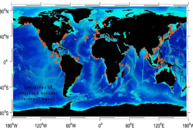
A comprehensive list of ISW observation sites has been compiled by Jackson (2004), with major study sites including the South China Sea (SCS) (Lien et al., 2005; Shaw et al., 2009; Ramp et al., 2004; Ramp et al., 2010), Massachusetts Bay (Scotti et al., 2007) and the

2

presence of a shallow thermocline (Shaw et al., 2009) and large scale surface currents, such as the Kuroshio in the SCS region.

Given the large amplitude and geographical range of ISWs in the oceans, it is unsurprising that their consequences are equally wide ranging. Physically, ISWs have been proposed as a mechanism for large scale sheer turbulence in the surface layer (Moum et al., 2003), and as a significant contributor to ocean heat fluxes (Shroyer et al., 2010). Geologically, Pomar et al. (2012) recently found that these waves can induce mobilization of bottom sediments

through strong bottom-current pulses by reviewing the global impact of ISWs on the sediment record. Additionally, Reeder et al. (2011) implicate ISWs as the primary cause of sediment bottom ripples in the South China Sea. ISWs also have a role to play in the

transport of nutrients; Pilot Whales have been known to follow in the wake of ISWs (Moore and Lien, 2007), and vertical fish migration following ISWs was recently observed off the

coast of Namibia (Kaartvedt et al., 2012).

3

of convergence and divergence on surface roughness, in near-surface currents (da Silva et al., 2011).

Numerous studies have applied statistical and observational methods to study ISWs in remote sensing images. The technique was first pioneered by Apel (1975) who compared the period of internal waves from direct cruise measurements in the New York Bight to the period observed in surface modulation, and found good agreement between the two. In the SCS, Zheng et al. (2007) used SAR images for a statistical analysis of internal wave

occurrence. Their study indicated interannual variability with higher frequencies of wave occurrence from April to July, peaking in June. Based on temperature measurements in the region, the authors found that the wave variability was associated with a shallower

thermocline in the summer months. They suggested that thermocline shoaling is an important factor in ISW generation. The higher frequency of surface modulations in the summer is therefore caused by the increased number of ISWs, which are more easily visible than internal waves. A full summary of internal wave remote sensing studies was recently conducted by Klemas (2012), illustrating that the physical parameters (wave speed,

4

Theoretical studies of solitary waves are nothing new; In 1895 Korteweg andde Vries first derived the mathematical properties of a “solition”, for surface waves (Konyaev et al., 1995). Further analytical solutions were derived by Lee and Beardsley (1974) and Hibiya (1986) using the Boussinesq approximations; Hibiya (1986) is the basis for the numerical

model used in this study (Shaw and Chao, 2006). Numerical models, such as the Regional Ocean Model system used by Buijsman et al. (2010), are now frequently utilized to

investigate internal wave properties. In addition, the SCS has been particularly well studied using process orientated models. Chao et al. (2007) examined the role of topographic height on westward propagation of internal tides, predicting that the topography in the region was capable of producing ISWs, as observed by Zhang et al. (2007). Shaw et al. (2009) discussed the role of thermocline shoaling on ISW generation, a primary reason for internal waves being more commonly observed to the west of the ridge in the SCS.

5

develop in large-amplitude internal tides produced by flow over a ridge. Wave packets then form at the wavefronts by nonlinear dispersion (Lee and Beardsley, 1974).

1.2 The Mascarene Plateau case study

Situated just to the east of Madagascar at 20°S 60°E, the Mascarene Plateau is comprised of an extensive range of banks and Islands (Figure 1.4), stretching approximately 2000 km. The South Equatorial Current (SEC), the major current in the South Indian Ocean, flows over the plateau almost entirely between the Saya de Malha and Nazareth banks (New et al., 2007). The flow direction here is predominately to the west (Figure 1.5) with speeds of around 50-70 cms-1 _{in the well mixed surface layer (depth of 50 – 100m). Tidal currents in the region} can reach 35 cms-1 _{with individual M}

2 and S2 components typically around 15 cms-1 (da Silva et al., 2011). From previous studies (Konyaev et al., 1995; New et al., 2007), the bottom

topography between the two banks consists of a ridge with a steep west slope and a gentle, shallower east slope (Figure 1.6).

6

the east, with a period corresponding to the semi-diurnal tidal cycle (12.42 hours). This result confirmed the findings of Morozov et al. (2009), that the temperature and currents fluctuated at the M2 tidal frequency. The shallow sill between the two banks is suggested by da Silva et al. (2011) as the primary generation site of the ISWs, based on tracing the

surface disturbances to their point of origin.

The presence of internal waves at the Mascarene Plateau has been confirmed

observationally by measuring thermocline displacement in the region (Konyaev et al., 1995). Using the temperature data collected along ship tracks across the ridge in March 1987 (Morozov and Vlasenko, 1996), Konyaev et al. (1995) concluded that internal waves appeared on both sides of the sill, and hypothesized two possible scenarios for their generation: (1) a hydraulic jump on the west side of the ridge, or (2) by the internal tide mechanism. In the first scenario, the combination of westward current (SEC) and maximum westward tidal flow result in a lee wave forming semi-diurnally. It is argued that the

7

due to the predominantly westward SEC. This also explains the increase in phase speed and maximum distance to the west of the sill as observed by da Silva et al. (2011).

In addition to the observed mode 1 waves generated at the ridge, Vlasenko and Morozov (1993) noted the existence of several other modes generated in the slope region when comparing numerical simulations with ADCP data. The authors concluded that at some distance from the ridge, the higher modes dissipate and the entire depth of the ocean is subjected only to first-mode oscillations. Konyaev et al. (1995) commented on the existence of mode 2 waves, suggesting they did not survive crossing the sill. Da Silva et al. (2011) found evidence for the existence of mode 2 waves, travelling eastward at a phase speed approximately 0.4 ms-1 _{in both the SAR images and thermocline displacement from} temperature records.

1.3 Internal wave energy flux

8

2003; Qian et al., 2010). In this study, the energy flux will be described in terms of the nondimensional slope parameter:

𝛾 =ℎ𝑥/𝛼 (1) where hx is the maximum slope of the topography and α is the slope of the internal wave beam (Garrett and Kunze, 2007). From linear wave theory, for waves of frequencyω_{, the}

slope of the wave beam can be defined as:

𝛼=

(

) (

)

/

f N

ω ω

 − − 

  (2)

where N is the buoyancy frequency and f is the Coriolis parameter. The slope parameter (γ)

can be defined as either supercritical (γ>1) or subcritical (γ <1). Bell’s solution (1975) for energy flux in an ocean of infinite depth is in the range 𝛾 ≪1 and is given by:

(

) (

)

2 2 2 2 2 2

0 0 0 1 /

F ∝ρU h N −ω − f ω (3)

Where ρ0is a reference density, h0 is the topographic height and U0is theamplitude of the

9

In a series of experiments between the interval 0 < 𝛾 < 1, Balmforth et al. (2002) show that enhancement in energy flux above Bell’s prediction followed a smooth and modest

increase, up to 14% larger for a gaussian bump as the slope parameter approaches 1. Petrelis et al. (2006) approximated the case in the supercritical range𝛾 > 1 using

knife-edge topography, in which the width of the ridge tends to 0 for a given height and 𝛾 →∞ (see Peacock et al., 2008). Their solution provided a rough estimate for more realistic supercritical ridges. They concluded that the radiative power of an internal wave increases monotonically with increasing slope parameter in the supercritical range. A recent

laboratory study by Dossmann et al. (2011) confirmed the validity of this trend, showing good agreement with energy flux values over a supercritical guassian ridge calculated theoretically and numerically (such as St. Laurent et al., 2003).

10

the Mascarene Plateau caused by the asymmetry of the topography, the mean surface current (New et al., 2007), or a combination of these factors? To what extent is one more important than the other?

Using a non-hydrostatic model, this study intends to replicate ISW generation over a series of two-dimensional ridges. While one slope remains supercritical, the other slope will cover both the subcritical and supercritical ranges. The contribution to the ISW energy flux from both sides of the topography is calculated to examine the role of asymmetrical ridge topography on ISW generation worldwide. The Mascarene Plateau is considered as a case study in this context, and surface currents are examined as an alternative hypothesis for the observed asymmetry in ISW occurrence.

This thesis is organized as follows: Chapter 2 describes the model configuration and the experiment setup. Chapter 3 presents the model results for a variety of topographical slopes ranging from a step function (γ → ∞) to a continental shelf (𝛾 →0). Chapter 4

11

2. Model description and experiments

2.1 Model Setup

For this study, the three-dimensional nonhydrostatic numerical model of Shaw and Chao (2006) is used, also previously employed in Chao et al (2007), Shaw et al. (2009) and Qian et al. (2010). The model solves the three-dimensional momentum, continuity, and density

equations with Boussinesq and rigid-lid approximations. The governing equations are:

2 2

2

0 0

1

2 _{H H}

D

p g A

Dt z

ρ

_ν

ρ

ρ

k u k u (4)

0

∇⋅ =u (5)

2 2 2 H H D K Dt z ρ _{= ∇ ρ κ+} ∂ ρ

∂ (6)

where u is the three-dimensional velocity vector (u, v, w) in the (x, y, z) coordinates, k’ isa unit vector pointing upward from the North Pole, k is the local upward unit vector,ρ is the

deviation of density from a reference density ρ0(1028 kg m

−3_{),Ω is the Earth’s rotation}

rate, and p is the pressure. The kinematic eddy viscosity and diffusivity are constant, so that AH = 106 m2/s, KH = 10 5 m 2s−1, ν= 1×10−4 m 2s−1, and κ= 0.1×10− 4 m 2s−1. Equation (5)

12

difference form of the governing equations and the solution procedure are described in detail in Shaw and Chao (2006).

The model domain is from x = −300 km to 300 km in the east-west direction and from z = −H

= −800 m at the bottom to 0 m at the surface. The horizontal and vertical grid sizes are 200

m and 10 m respectively. A rigid lid is used at the surface for computational efficiency which, due to the relatively small phase speed of baroclinic waves compared to that of the

barotropic waves, should not affect the amplitude of internal waves over the ridge

significantly. In the y direction, two grid cells are used with a periodic boundary condition; no y-variation is introduced, so that although the model is three-dimensional, this study is in the two dimensional x and z space.

Flow over the ridge is forced by the oscillating barotropic M2 tide and a steady current (Uc). The velocity in the x-direction is given by:

𝑈 =𝑈𝑐+ 𝑈0𝑠𝑖𝑛 𝜔𝑡 (7)

where 𝜔= 2π/12.42 rad hr-1 _{= 8.86 x10}-4 _{rad s}-1

13

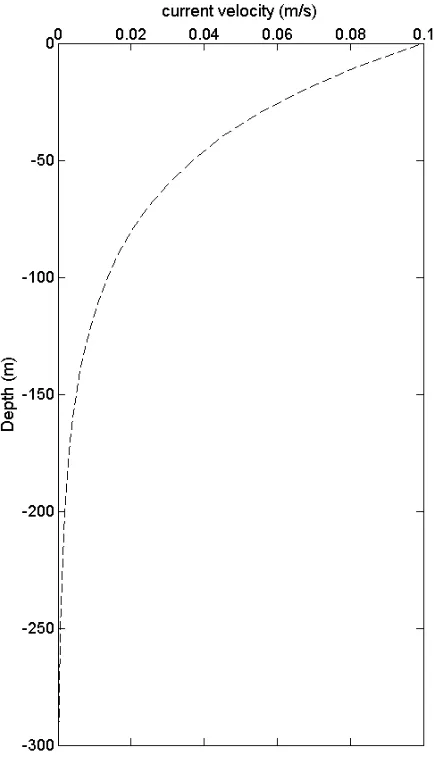
The steady current Uc is represented either as a mean flow, constant with depth, or as a surface current decaying exponentially with depth:

𝑈𝑐 =𝑈𝑚𝑒(𝑧/𝑑) (8) where Um is the mean surface current and d = 50 m is the e-folding depth (Figure 2.1). The perturbation density ρ′is

ρ′

(

)

( )

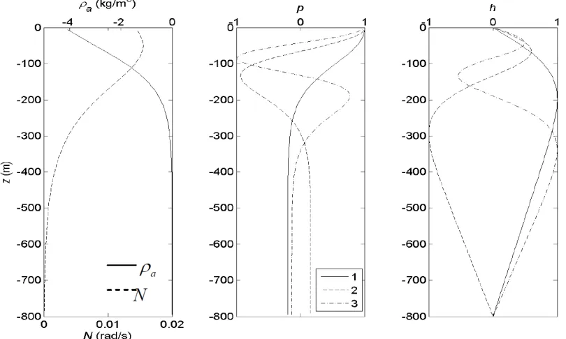
The ambient stratification ρa(z) is given by

( )

2 a z z z D ρ ρ = −∆ _ + _ − __  

  (10)

where ∆ρ is the scale of density perturbation. The thermocline is centered at depth z0 (=

−50 m) with thickness D (= 120m). The buoyancy frequency derived from (10) is

(

)

1/ 2

1/ 2 _{0 0}

0 max

0

sech sech

2

a

z z z z

g

N d dz N

D D D

ρ ρ ρ ρ  ∆   −   −  = −_ _ =_{   }= _{ }    

  . (11)

The maximum buoyancy frequency Nmax occur s at z = z0, and Nmax =N0 =0.015 rad/sfor

3 6 kg/m ρ

∆ = and 3

0 1028 kg/m

ρ = . Figure 2.2 shows the modal decomposition for this

stratification. Mode-1 waves associated with (11) have zero horizontal velocity and

14

The phase speed of the mode-1 wave is 1.52 ms-1 forNmax = N0, and is proportional to Nmax

in other experiments. For semidiurnal tides, the internal wave energy is negligible below z = −700 m. Extending the depth of the model to below 800m should not therefore affect

internal wave generation significantly.

2.2 Experiment parameters

In this study, ISWs will be described in terms of both their overall energy (E) and normalized

energy flux (F’). The baroclinic velocity u′ ≡

(

)

depth-averaged horizontal velocity from the total velocity u, is used in the equation for the perturbation kinetic energy density:

0

(

)

1

2

K

=

ρ

u

′

+

v

′

+

w

′

and the perturbation potential energy density is

2 2 2 0

1

2

g

P

N

ρ

ρ

′

=

15

The internal wave energy flux is p′ ′u ,where p′is the perturbation pressure. From Nash et

al. (2005) p’ is obtained by subtracting the depth-averaged pressure 𝑝 from hydrostatic

pressure p:

p x z t′( , , )= p x z t( , , )−p x t( , ) (14)

where the depth averaged pressure is given by

(15)

where zb is the z-coordinate for the bottom.

In this study, the vertically integrated horizontal energy flux given by

𝐼 =∫ 𝜌0 ′𝒖′_𝑑𝑧

𝑧𝑏 (16)

is averaged over an area A, following a wave beam in time and space (Figure 2.3). The spacial average of A is one wavelength in the x-direction (67.96km) and the temporal average is one wave period (12.42 hours). The wavelength is calculated using the theoretical phase speed of the internal wave, 1.52 ms-1. The baroclinic energy flux is calculated

𝐹 =𝐼������(𝐴) (17) where the overbar represents averaging over A.

0 0 1 '( , , ) b z z b

p dz p x z t gdz

z

 

 

 ′ ′

16

Qian et al. (2010) showed that a normalization scheme may be applied to F. The

nondimensional horizontal energy flux (F’) is defined as

𝐹

=

𝜌𝐻𝑈0𝑁�𝑟ℎ0 (18) Where N�r is the averaged buoyancy frequency over the depths of the ridge ho

𝑁�

=

∫

𝑁𝑑𝑧

2.3 Ridge design and experimental setup

The tidal flow over idealized topography, described in Eq. (7), forms the basis for a series of experiments. Each experiment consists of a fixed slope on the west side of the ridge, a plateau width of 20 km, and a variable east slope. The ridge is described by the Witch-of-Agnesi function

(

)

2

( ) m/ 1 /

h x h _ x L _

 

= + (20)

where hm is the maximum height, and L is the half-width of the slope. In this study, hmis fixed at 600 m, and L is varied to change the maximum slope of the ridge on the east side, while being fixed at L=15 km on the west side.

The maximum slope, h’x = (33/2/8)hm/L, is at x = 3-1/2 L. The ridge is shifted vertically for

17

slope of the ridge does not change with the vertical shift. The model setup is shown in Figure 2.4. Each experiment is Table 2.1 varies in L only on the east (right) side of thee ridge. For example, experiment 1Dcorresponds to a ridge of L= 15km for the east slope. The experiment 1G is based on the Mascarene Plateau, following the measurements of the local topography by New et al. (2007). An additional set of experiments, detailed in Table 2.2 are used to examine other potential impacts on internal wave generation, explicitly the latitude of the ridge location, the plateau width and the surface current velocity.

In this study, the wave slope in eq. (1) is represented by the average wave slope between zt = -200 m and 0 m

𝛼

=

𝑡|

∫

(

𝜔2−𝑓2 𝑁2−𝑓2

)

1 2

0

𝑧𝑡

𝑑𝑧

18

3. Model Results

3.1 Normalized energy flux

The normalized baroclinic energy flux, F’ is calculated on both sides of the ridge as described by eq(16) – (18) and shown in Figure 3.1. For all cases, the wave energy flux is slightly higher on the side of the ridge with a steeper slope, with the approximately equal

symmetrical case (1D, γ=2.36) being the only exception to this. Over the whole range of experiments, F’ increases substantially with the slope parameter for the east slope. Three separate categories are defined: subcritical, transitional and supercritical.

In the subcritical range γ<0.75 (1J, 1K and 1M, enclosed by a rectangular box), the flux is at a minimum value on both sides of the topography, F’ ≈ 0.2. There is no significant difference observable between the cases in this range. However, energy flux in the westward

19

than the west slope. The cases in this range (1D, 1C, 1B) are enclosed in an ellipse and like the subcritical cases, have similar characteristics. The value of F’ for eastward propagating waves of the two end member cases (1A and 1M) are shown as two black horizontal lines, bounding the supercritical and subcritical regions. These two cases do not share the properties of the conventional topography cases, as will be discussed in due course.

3.2 Internal wave energy

20

of the ridge. However, the wave beams propagating toward the centre of the ridge are out of phase with the outward propagating waves and therefore do not contribute as much energy.

ISWs are characterized by oscillations in the density field, with a sharp leading edge and strong downward flow. On leaving the ridge, a mode one wave forms and develops into an ISW on either side of the topography, indicating that the slopes on both sides of the ridge are supercritical. In experiment 1A (Figure 3.2a), the step function on the right side of the ridge generates a large amount of energy. Most of the energy propagates to the east in a wide wave beam. A strong ISW, with a sharp downward leading edge forms at

approximately 120 km from the origin. The weaker narrower wave beam to the west of the ridge also forms an ISW. It is weaker than its counterpart to the east, with a shallower leading edge and smaller amplitude.

21

due to the difference in energy contributed from the right slope. ISWs are still present on both sides. However, the energy in the ISW on the east side is comparable to that on the west side and is less than in Figure 3.2a because of the less steep right slope. In the final panel Figure 3.2c, the energy density generated on both sides of the ridge has decreased, with a wave beam nearly invisible at the right topography slope. The maximum energy density at the surface is also lower on both sides and the ISW packets that appear are less intense.

Figure 3.3 compares the energy density for cases 1H (transitional), 1K and 1M (subcritical). Comparing Figure 3.3a to Figure 3.2c, the energy density is much lower than in 1E. Wave beams are generated only on the left side of the ridge and propagate toward both

directions. No ISWs form on either side. The decrease in maximum slope on the right side of the topography is observed to have a significant impact on both sides of the model domain. This trend is continued in Figure 3.3b. The internal waves still propagate from the left side of the ridge in the subcritical case 1K with slightly smaller peak energy values than that in 1H (8 J/m3). Figure 3.3c shows the weak energy generation associated with case 1M, approximately eight times smaller than case 1C. The continental shelf topography

22

broadly symmetrical, with some modification to the wave beam on the east side due to the shelf topography.

The experiments with varying slope on one side of the ridge indicate that wave beams are generated only from supercritical slopes. When both slopes are supercritical, wave beams form on both sides of the ridge and strong internal waves propagate away from the ridge in both directions. If the slope on one side of the ridge is transitional or subcritical, the

strength of the internal wave is greatly reduced. Waves are now contributed only from the supercritical side of the ridge but internal waves propagating in both directions are of comparable strength.

3.3 Baroclinic energy flux

The vertically integrated horizontal energy flux is displayed as a function of x in Figure 3.4 for the four supercritical cases 1A, 1B, 1C and 1D. The transitional and subcritical cases are similarly displayed in Figure 3.5 and Figure3.6 respectively. The flux is averaged over the same tidal period as in Figures 3.2. Negative (positive) values indicate a westward

23

The flux across the ridge is close to zero in all four supercritical cases, with a small westward flux in case 1B and 1C due to the right ridge slope being steeper. To the west of the ridge, the flux reaches a maximum value at the horizontal extent of the ridge topography, x ≈ - 30 km. This maximum value is similar for 1B, 1C and 1D, suggesting the westward flux is independent of the eastward slope in this supercritical region. The westward flux is slightly less in the case 1A, implying there is some energy dissipation caused by the step topography on the right of the ridge. ISW packets of similar intensity form at x ≈ -150 km. To the right of the plateau, the varying slope width changes the lateral extent of the topography. This is observed in the location of the maximum flux, which moves further to the right of the domain as slope width increases from 0 to a finite value. Cases 1B, 1C and 1D are

24

For the cases with a transitional slope on the right of the ridge (Figure 3.5), the flux over the plateau is positive. Energy from the left side of the topography contributes to the wave beam on the right side. The magnitude of the flux crossing the ridge is inversely related the slope parameter of the right slope, with substantially higher flux contributed in case 1I than in 1E. The westward flux increases to a maximum value at the same location for all

transitional cases as 1D (x=- 30km), and ISWs are observed for the two cases closest to the supercritical range, 1E and 1F. As in Figure 3.4, the eastward flux in the supercritical cases increases to a maximum at the lateral extent of the topography. In the transitional cases however, there is a decrease to a lower flux value after the peak flux. Both the maximum flux value and the extent of the decrease are positively related to the east slope parameter. For example, flux in case 1F peaks at 1230 W/m on the east side of the domain, before decreasing to 1112 W/m at 150 km. The flux in case 1H peaks at 998 W/m, before

decreasing to 758 W/m at 150 km. As with the westward flux, ISWs form in cases 1E and 1F whereas the others do not.

-25

470 W/m at x = 30 km. The flux across the plateau is constant in all subcritical cases. The eastward flux from the west side of the ridge to the east side is higher than in either the transitional or supercritical cases. Furthermore, the cross plateau flux (420 W/m) is approximately the same as the westward flux from the left edge of the topography. On crossing the right slope, the flux increases, with a larger increase in the case of a steeper slope. As with the transitional cases, this flux quickly decreases to a lower value. The steady flux value reached at x=150 km is slightly lower than the contribution from the supercritical left side of the ridge, suggesting the subcritical right side dissipates more energy than it contributes. In this respect, 1M does not agree well with the other subcritical cases. The energy flux on both sides of the ridge is much smaller, and remains constant away from the topography. No ISW packets are generated in any of the subcritical cases.

To summarize, topography with two supercritical slopes will not generate significant net energy flux across the ridge, but will generate large internal waves propagating away from the topography, which develop into ISWs. A ridge with one supercritical slope and one subcritical slope will generate energy flux of approximately equal strength in both

26

plateau flux from the steeper side increases as the slope parameter on the other side decreases. Dissipation reduces the flux leaving the less steep slope, resulting in a small east-west asymmetry in energy flux. ISW packets are observed in this range only for γ > 1.5.

3.4 Additional experiments

In addition to the variation in internal wave energy caused by decreasing the slope parameter on one side of the ridge, a number of supplementary experiments have been

carried out (Table 2.2). Here, three model parameters are examined: the width of the topography plateau, the application of a steady current and the latitude.

3.4.1 Plateau Width

Case 1D is compared with experiment 1a from Qian et al. (2010), referred to as 2A for the purposes of this study. The two model setups differ only in the ridge design; while both experiments have symmetrical slopes of L = 15km, the 1D case has a plateau width of 20 km, unlike 2A which has no plateau (bell shaped ridge).

27

topography, x=0 km in a steep vertical wave beam. The surface maxima of 2A and 1D differ due to this difference in generation site. Averaged over the tidal period, the energy density is more evenly distributed in 1D with lower peak values than in 2A where the wave beam first reflects from the surface. However in 1D the ISW formed on both sides of the ridge is stronger, with a steeper wave front, due to the combination of internal wave energy from both sides of the ridge plateau.

28 3.4.2 Steady current

Figure 3.9 compares the energy density field for 1D (Figure 3.9b)with and without a steady westward current. Figure3.9a shows case 2B, where a westward steady barotropic mean flow has been applied throughout the water column and Figure 3.9c shows case 2C where the current decays exponentially from the sea surface with a decay scale of 50m. The transport in each case is given in Table 2. In Figure 3.9a, the wave seems stronger on the ridge top but ISWs formed away from the ridge are weaker. In Figure 3.9c the wave beam is wider than in Figure 3.9b, with a maximum on the west topographic slope not observed in 1D. The energy at the surface is slightly diminished by the mean flow and the leading edge of the ISW is shallower on the west side of the domain. The most significant differences between 1D and 2C in Figure 3.9c are in the surface layer, z > - 100m. An increase in the peak energy is shown at each instance the internal wave is reflected downward by the surface. The strength of the ISW increases on both sides of the domain. There is no significant impact to the internal wave energy field beneath z = - 100m.

29

observable in the large scale oscillations in both positive and negative fluxes. In general, for the given transport values, the three experiments have similar energy flux away from the ridge. A mean current such as the SEC will not have a significant impact on the energy flux of internal waves.

3.4.3 Latitude

30

increases. 2F is approaching the critical latitude at 75°S, beyond which internal waves will not propagate.

4. Mascarene Plateau

Here the 1G case is studied in more detail. This experiment is designed to match the

31

Figure 4.2 plots the energy density field in the x-z plane. Energy is generated on both sides of the topography. Beneath the strongly stratified thermocline (z=200m), the wave beam from the west slope of the ridge is stronger. Like the subcritical range, the westward wave is also stronger than its eastward counterpart. The maximum energy value occurs at

approximately x=0 km, suggesting that internal wave energy from both sides of the ridge is coalescing at this point, with stronger propagation to the west.

32

forms then is of an internal wave generated on the west side of the topography, with stronger energy flux in the west direction. The east internal wave is reinforced by energy from the east side of the topography, with some energy dissipating over the subcritical east ridge slope. ISWs form at a distance greater than 200 km from the centre of the plateau.

4.2 Mode 2 waves

Both Konyaev et al. (1995) and da Silva et al. (2011) commented on the existence of mode 2 waves at the Mascarene Plateau, citing both SAR images and thermocline displacement records. The model does not reproduce these mode 2 waves in experiment 1G, but they are observable in the most supercritical case. A contour plot of the vertically integrated

33

5. Discussion

Internal waves form as a barotropic tide moves over a steep ridge, propagating away from the topography as a wave beam. If the internal wave amplitude is large enough, it will develop into an ISW. For a given tide, the energy required to form internal waves is dependent on the ridge slope exceeding a critical threshold; regions of critical slope act as sources of energy flux in the lower modes (Garrett and Kunze 2007). In this study, the same tidal flow produced internal waves of varying energy, depending on the critical value of the slope parameter on one side of the ridge, where the other slope remained constantly supercritical (γ=2.6).

In the supercritical range, wave beams propagate vertically from both ridge slopes,

becoming horizontal as the water column becomes less stratified. The wave beam splits into eastward and westward components, one moving away from the topography and the other toward the center of the domain. The two wave beams moving in the same direction are not in phase, due to the plateau width between the two slopes. A ridge with a flat plateau generates more energy flux than a bell shaped ridge of the same slope parameter,

34

In the transitional range a vertical wave beam is generated only on the supercritical ridge slope. The energy flux at the other slope is mainly over the flank of the ridge, rather than as a concentrated wave beam (Figure 4b Qian et al. 2010). The normalized energy flux F’ decreases monotonically with slope parameter on both sides of the model domain, as less energy is contributed to the wave beam developed on the supercritical side of the ridge. A similar result was obtained by Khatiwala (2003) for a bell shaped ridge of fixed height with varying wave slope α. Energy crosses from the supercritical side to the subcritical side. As the right slope parameter decreases, the left supercritical slope contributes more flux to the wave propagating to the right. In the subcritical range, the energy flux in both directions reaches a minimum, whereas a large flux crosses the ridge. Energy is now dissipated over the subcritical slope, and the flux in each direction is approximately four times less than in the supercritical range.

35

greater slope parameter. Regardless of the difference between the slope parameters on each side of the ridge, the difference in vertically integrated energy flux was approximately 100 W/m. This suggests that this energy dissipated as the internal wave crossed the plateau to the right hand side of the ridge.

In the case of the Mascarene Plateau, the topography in the region is established to be a crucial factor in the asymmetry of internal wave observations. The results of the case study are qualitatively similar to those reported by da Silva et al. (2011) with a stronger ISW forming to the west of the ridge. As in observations, the internal waves are generated by the lee wave mechanism on the west side of the ridge. The phase speed and wavelength of the internal waves is larger in the observations than in the model, as the tidal velocity was reduced here for model stability, and to allow comparisons with Qian et al. (2010).

Increasing the surface current velocities to match the conditions at the Mascarene Plateau destabilizes the simulation. Strong interactions with the bottom topography created large energy fluxes near the ridge topography. This made it difficult to estimate the internal wave energy flux, and the results are not included here.

36

case 1A, where the flow becomes supercritical for mode 2 waves (Stastna and Peltier 2005). The idealized 2-D topography of the ridge was based on the results of New et al. (2007). This study did not attempt to model realistic topography in the Mascarene Plateau region, using instead an idealized version based on the calculated slope angle and plateau width of the ridge. Imprecise knowledge of ocean bottom topography is a major source of error for this study, and for the accurate modelling of internal waves everywhere (Llewellyn Smith and Young 2003), particularly given the high sensitivity of internal wave energy flux to slope steepness.

37

6. Conclusion

A series of experiments are carried out using a three-dimensional nonhydrostatic numerical model to examine the impact of asymmetrical topography on internal wave energy. Internal waves are shown to be less energetic on both sides of the domain as the slope on one side becomes smaller, despite a supercritical slope on one side of the ridge. Although the overall energy generated by the topography decreases markedly with decreasing slope parameter, the difference in flux between the eastward and westward propagating waves remains small in the transitional to subcritical range γ <2, with energy on the most critical ridge slope being slightly higher. Energy dissipation as the internal wave crosses the ridge is concluded to be the cause of this discrepancy. In the subcritical range, the energy flux across the topography is higher, as less wave energy is generated from the other slope. Topography with a flat plateau is also shown to generate larger internal waves than a bell shape ridge of the same supercritical slope value, due to the generation and interaction of multiple wave beams.

38

internal waves in the region, for an idealized two-dimensional ridge. Applying a steady current, designed to simulate the westward SEC in the region, however showed no

significant difference to the vertically integrated internal wave flux but a noticeable increase in the energy at the surface if the current is surface intensified as is the case of the

Mascarene Ridge. Previous studies (da Silva et al. 2011, Konyaev et al. 1995) have suggested this as the cause for the asymmetry of internal waves in the region. This study presents a combination of the topographic asymmetry and the SEC as the primary cause.

This result has implications for internal wave generation over complex topography,

39

REFERENCES

Apel, J. R., H. M. Byrne, J. R. Proni, and R. L. Charnell (1975), Observations of oceanic internal and surface-waves from earth resources technology satellite, Journal of Geophysical Research, 80(6), doi: 10.1029/JC080i006p00865.

Balmforth, N. J., G. R. Ierley, and W. R. Young (2002), Tidal conversion by subcritical topography, J. Phys. Oceanogr., 32(10) doi: 10.1175/1520-0485(2002)032

Bell, T. H. (1975), Lee Waves in stratified flows with simple harmonic time-dependence, J. Fluid Mech., 67, doi: 10.1017/S0022112075000560.

Brandt, P., A. Rubino, W. Alpers, and J. Backhaus (1997), Internal waves in the strait of messina studied by a numerical model and synthetic aperture radar images from the ERS 1/2 satellites, J. Phys. Oceanogr., 27(5), 648-663, doi: 10.1175/1520-0485

Buijsman, M. C., J. C. McWilliams, and C. R. Jackson (2010), East-west asymmetry in nonlinear internal waves from Luzon Strait, Journal of Geophysical Research-Oceans, 115, C10057, doi: 10.1029/2009JC006004.

Cacchione, D. and L. Pratson (2004), Internal tides and the continental slope, Am. Sci., 92(2), 130-137, doi: 10.1511/2004.46.924.

Chavanne, C., P. Flament, D. Luther, and K. -. Gurgel (2010), The surface expression of semidiurnal internal tides near a strong source at hawaii. Part II: Interactions with mesoscale currents, J. Phys. Oceanogr., 40(6), 1180-1200, doi: 10.1175/2010JPO4223.1. Chao, S., D. Ko, R. Lien, and P. Shaw (2007), Assessing the west ridge of luzon strait as an internal wave mediator, J. Oceanogr., 63(6), 897-911, doi: 10.1029/2003G1A19077.

da Silva, J. C. B., A. L. New, and J. M. Magalhaes (2011), On the structure and propagation of internal solitary waves generated at the Mascarene Plateau in the Indian Ocean, Deep-Sea Research Part I- , 58(3), 229-240, doi: 10.1016/j.dsr.2010.12.003.

40

Garrett, C. and E. Kunze (2007), Internal tide generation in the deep ocean, Annu. Rev. Fluid Mech., 39, doi: 10.1146/annurev.fluid.39.050905.110227.

Hibiya, T. (1986), Generation mechanism of internal waves by tidal flow over a sill, Journal of Geophysical Research-Oceans, 91(C6), 7697-7708, doi: 10.1029/JC091iC06p07697. Jackson C. R. (2004), An Atlas of Internal Solitary-like Internal Waves, Global Ocean Assoc., Alexandria, Va.

Kaartvedt, S., T. A. Klevjer, and D. L. Aksnes (2012), Internal wave-mediated shading causes frequent vertical migrations in fishes, Mar. Ecol. -Prog. Ser., 452, 1-10, doi:

10.3354/meps09688.

Khatiwala, S. (2003), Generation of internal tides in an ocean of finite depth: analytical and numerical calculations, Deep-Sea Research Part I, 50(1), doi:

10.1016/S0967-0637(02)00132-2.

Klemas, V. (2012), Remote sensing of ocean internal waves: an overview, J. Coast. Res., 28(3), 540-546, doi: 10.2112/JCOASTRES-D-11-00156.1.

Konyaev, K., K. Sabinin, and A. Serebryany (1995), Large-amplitude internal waves at the Mascarene Ridge in the Indian ocean, Deep-Sea Res. Part I, 42(11-12), 2075, doi:

10.1016/0967-0637(95)00067-4.

Kurkina, O. E. and T. G. Talipova (2011), Huge internal waves in the vicinity of the

Spitsbergen Island (Barents Sea), Natural Hazards and Earth System Sciences, 11(3), doi: 10.5194/nhess-11-981-2011.

St. Laurent, L., S. Stringer, C. Garrett, and D. Perrault-Joncas (2003), The generation of internal tides at abrupt topography, Deep-Sea Research Part I , 50(8), doi: 10.1016/S0967-0637(03)00096-7.

Lee, C. and Beardsley, R.C. (1974), Generation of long nonlinear internal waves in a weakly stratified shear-flow, Journal of Geophysical Research, 79(3), 453-462, doi:

10.1029/JC079i003p00453.

Lien, R. C., T. Y. Tang, M. H. Chang, and E. A. D'Asaro (2005), Energy of nonlinear internal waves in the South China Sea, Geophys. Res. Lett., 32(5), 1A5615, doi:

41

Maxworthy T. (1979) A note on the internal solitary waves produced by tidal flow over a three dimensional ridge, J. Geophys. Res., 84,338-346, doi: 10.1029/JC084Ic01P00338 Moore, S. E. and R. Lien (2007), Pilot whales follow internal solitary waves in the South China Sea, Mar. Mamm. Sci., 23(1), 193-196, doi: 10.1111/j.1748-7692.2006.00086.x. Morozov, E. G. and V. I. Vlasenko (1996), Extreme tidal internal waves near the Mascarene ridge, J. Mar. Syst., 9(3-4), doi: 10.1016/S0924-7963(95)00042-9.

Morozov, E. G., L. V. Nechvolodov, and K. D. Sabinin (2009), Beam propagation of tidal internal waves over a submarine slope of the Mascarene Ridge, Oceanology, 49(6), 745-752, doi: 10.1134/S0001437009060010.

Moum, J., D. Farmer, W. Smyth, L. Armi, and S. Vagle (2003), Structure and generation of turbulence at interfaces strained by internal solitary waves propagating shoreward over the continental shelf, J. Phys. Oceanogr., 33(10), 2093-2112, doi: 10.1175/1520-0485(2003) Nash, J.D., Moum, J. (2005) River plumes as a source of large-amplitude internal waves in the coastal ocean. Nature437, 400-403. doi: 10.1038/nature03936

New, A. L., S. G. Alderson, D. A. Smeed, and K. L. Stansfield (2007), On the circulation of water masses across the Mascarene Plateau in the South Indian Ocean, Deep-Sea Research Part I, 54(1), 42-74, doi: 10.1016/j.dsr.2006.08.016.

Peacock, T., P. Echeverri, and N. J. Balmforth (2008), An experimental investigation of internal tide generation by two-dimensional topography, J. Phys. Oceanogr., 38(1), doi: 10.1175/2007JPO3738.1.

Petrelis, F., S. L. Smith, and W. R. Young (2006), Tidal conversion at a submarine ridge, J. Phys. Oceanogr., 36(6), doi: 10.1175/JPO2879.1.

Pomar, L., M. Morsilli, P. Hallock, and B. Badenas (2012), Internal waves, an under-explored source of turbulence events in the sedimentary record, Earth-Sci. Rev., 111(1-2), 56-81, doi: 10.1016/j.earscirev.2011.12.005.

Qian, H., P. Shaw, and D. S. Ko (2010), Generation of internal waves by barotropic tidal flow over a steep ridge, Deep-Sea Research Part I , 57(12), 1521-1531, doi:

42

Quaresma, L. S., J. Vitorino, A. Oliveira, and J. da Silva (2007), Evidence of sediment

resuspension by nonlinear internal waves on the western Portuguese mid-shelf, Mar. Geol., 246(2–4), 123-143, doi: 10.1016/j.margeo.2007.04.019.

Ramp, S. R., T. Y. Tang, T. F. Duda, J. F. Lynch, A. K. Liu, C. S. Chiu, F. L. Bahr, H. R. Kim, and Y. J. Yang (2004), Internal solitons in the northeastern South China Sea - Part I: Sources and deep water propagation, IEEE J. Ocean. Eng., 29(4), doi: 10.1109/JOE.840839.

Ramp, S. R., Y. J. Yang, and F. L. Bahr (2010), Characterizing the nonlinear internal wave climate in the northeastern South China Sea, Nonlinear Processes in Geophysics, 17(5), doi: 10.5194/npg-17-481-2010.

Reeder, D. B., B. B. Ma, and Y. J. Yang (2011), Very large subaqueous sand dunes on the upper continental slope in the South China Sea generated by episodic, shoaling deep-water internal solitary waves, Mar. Geol., 279(1-4), 12-18, doi: 10.1016/j.margeo.2010.10.009. Scotti, A., R. C. Beardsley, and B. Butman (2007), Generation and propagation of nonlinear internal waves in Massachusetts Bay, Journal of Geophysical Research-Oceans, 112(C10), C10001, doi: 10.1029/2007JC004313.

Shaw, P. and S. Chao (2006), A nonhydrostatic primitive-equation model for studying small-scale processes: An object-oriented approach, Cont. Shelf Res., 26(12-13), 1416-1432, doi: 10.1016/j.csr.2006.01.018.

Shaw, P., D. S. Ko, and S. Chao (2009), Internal solitary waves induced by flow over a ridge: With applications to the northern South China Sea, Journal of Geophysical Research-Oceans, 114, C02019, doi: 10.1029/2008JC005007.

Shroyer, E. L., J. N. Moum, and J. D. Nash (2010), Vertical heat flux and lateral mass transport in nonlinear internal waves, Geophys. Res. Lett., 37, 1A8601, doi:

10.1029/2010G1A42715.

Smith, S. G. L. and W. R. Young (2003), Tidal conversion at a very steep ridge, J. Fluid Mech., 495, doi: 10.1017/S0022112003006098.

43

Vlasenko, V. I. and E. G. Morozov (1993), Generation of Semidiurnal Internal Waves Over a Submarine Ridge, Okeanologiya, 33(3).

Vlasenko, V. and K. Hutter (2002), Numerical experiments on the breaking of solitary internal waves over a slope-shelf topography, J. Phys. Oceanogr., 32(6), 1779-1793, doi: 10.1175/1520-0485

44 Table 2.1: List of experiments.

Experiment name Variable slope width (L in

km) Slope parameter (γ)

1A 0 Inf

1B 10 3.54

1C 12 2.95

1D 15 2.36

1E 18 1.97

1F 23 1.57

1G 30 1.18

1H 38 0.93

1I 45 0.79

1J 60 0.59

1K 78 0.45

1L 130 0.27

45 Table 2.2: List of secondary parameter experiments.

Experiment name Base experiment Variation from base experiment

2A 1D Plateau width = 0 km,

20km in original case

2B 1D Additional 2.5 cm/s

barotropic mean flow

2C 1D Additional 10 cm/s

current decaying exponentially with depth

2D 1D Latitude = 0°, 12.5° in

original case

2E 1D Latitude = 20°

46

47

48

49

50

51

52

53

54

55

Figure 2.4. The model configuration. Contours show the background density field averaged over 12 hours for case 1D. The model is forced by a semidiurnal tide

56

57

Figure 3.2 Internal wave energy density (J/m3_{) averaged over one tidal cycle 49.70 – 62.10} hours, for L equal to (a) 0 km (b) 12 km and (c) 18 km. The width of the slope on the left is 15 km. The contour interval in all panels is 1 J/m3

a) 1A

b) 1C

c) 1E a) 1A

b) 1C

a) 1A

58

Figure 3.3. Same as Figure 3.2 but for L equal to (a) 38 km (b) 78 km and (c) infinity. The contour interval in the top two panels is 1 J/m3 _{and 0.1 J/m}3 _{in the bottom panel}

a) 1H

b) 1K

59

60

61

62

Figure 3.7. Internal wave energy density (J/m3_{) for (a) 1D and (b) 2A averaged over one tidal} cycle, 49.70 – 62.10 hours. The contour interval is 1 J/m3

(a) 1D

63

Figure 3.8. Vertically integrated horizontal energy flux (W/m) as a function of x for

64

Figure 3.9 Internal wave energy density (J/m3) for (a) 2B (b) 1D and (c) 2C. The energy density is averaged over one tidal cycle, 49.68 – 62.10 hours. The contour interval is 1 J/m3

a) 2B

b) 1D

65

66

67

68

69

70