Dynamic Bandwidth Optimization for Coordinated Arterial.

ABSTRACT

KIM, SANGKEY. Dynamic Bandwidth Optimization for Coordinated Arterial. (Under the direction of Dr. Billy M. Williams and Dr. Nagui M. Rouphail.)

Urban traffic congestion problems continue to be an important focus of fundamental and applied research. Economic vitality and environmental sustainability will be directly impacted by the quality of the innovative solutions brought forth to address issues of travel delay and wasted fuel consumption. Signalized urban arterials are a key component of overtaxed urban transportation networks.

A commonly used strategy for improving mobility along signalized arterials is coordination of neighboring intersections to minimize stops by maximizing the duration of green bands, otherwise known as arterial bandwidth. Signal coordination has been

researched, developed, and refined for five decades. In contrast to traditional methods based on analysis of programmed green times, a dynamic bandwidth analysis method is presented that reproduces actual dynamic bandwidth durations using closed loop signal data to assess the performance of semi-actuated coordinated arterial streets.

In this study, the author introduces 1) an enhanced MAXBAND formulation, 2) dynamic bandwidth characteristics, and 3) dynamic bandwidth optimization method.

seminal MAXBAND papers. The test result supports that the new formulation is consistent with the original MAXBAND formulation in cases where over constraint and suboptimality are not an issue and that the new formulation provides an optimal solution in cases where the original formulation performs suboptimality due to over constraint of the bandwidth ratio.

Although the newer MILP formulations, MULTIBAND, MULTIBAND-96, and AM-BAND, include increasingly innovative objective functions and constraints compared to the original MAXBAND MILP, all the MAXBAND-related models have similar constraints incorporating the directional bandwidth target value. Therefore, the modified objective function and constraints in the new formulation can be used to revise the formulations for all of the MAXBAND family of optimization models such as MULTIBAND, MULTIBAND-96, and AM-BAND.

In addition, this study shows real world dynamic bandwidth characteristics. Detailed analysis at three arterial sites revealed that coordinated green time distributions are complex and multi-modal and cannot be represented by a single statistic. Dynamic bandwidth analysis confirmed that programmed green bandwidth consistently underestimates the size of the actual dynamic bandwidth, and exhaustive search results highlighted the potential for further improvements in coordination.

Finally, the author provides dynamic bandwidth optimization methods for improving arterial coordination quality. The provided methods are 1) exhaustive search method by developed LP and 2) linear programming. The exhaustive search method can provide the complete feasible solution space so it is possible to easily understand each offsets

archived signal log data regarding phase start and end times in each cycle in both directions. Those data are used to optimize the offsets that maximize the variable system bandwidth across multiple cycles constituting a coordination plan period. The formulation can also be used to optimize signal offsets using programmed (fixed) green durations at each

intersection. The proposed formulation offers five significant enhancements compared to traditional methods. The optimal offset solutions are tested in the field, and the results support the effectiveness of provided dynamic bandwidth optimization method.

Dynamic Bandwidth Optimization for Coordinated Arterial

by Sangkey Kim

A dissertation submitted to the Graduate Faculty of North Carolina State University

in partial fulfillment of the requirements for the degree of

Doctor of Philosophy

Civil Engineering

Raleigh, North Carolina

2014

APPROVED BY:

_______________________________ ______________________________ Billy M. Williams, Associate Professor Nagui M. Rouphail, Professor

Committee Co-Chair Committee Co-Chair

________________________________ ________________________________

DEDICATION

BIOGRAPHY

Sangkey Kim was born in Andong, South Korea on February 19, 1977. He entered Chung-Ang University in 1997 and earned a bachelor’s degree in civil engineering. Mr. Kim studied urban engineering as a master’s student. He focused on the transportation planning area especially future demand forecasting and traffic assignment methods. After earning his master’s degree, he worked for the Korea Transport Institute (KOTI) for two years. As a transportation planning researcher, Mr. Kim conducted several of pre-feasibility studies for freeway, railroad and subway system construction plan evaluation for the Korean

ACKNOWLEDGMENTS

First and foremost, I would like to express gratitude to my advisors, Dr. Nagui Rouphail and Dr. Billy Williams, for their guidance and counsel throughout my research and preparation for this dissertation. They gave me invaluable lessons in life and research as well as continuous support for my research during past four and one half years.

I would also like to express my appreciation to Dr George List and Dr Yahya Fathi who were willing to be my committee member and gave precious advice for my dissertation.

I would also like to thank my friend Dr. Ali Hajbabaie who provided me with advice and helped guide my research. His helping attitude and devotion supported me all the time.

I also appreciate my friend, Chang Beak, who is a signal engineer with NCDOT. He taught me from A to Z about the NCDOT signal system. Without his help, I could not have accomplished this dissertation.

TABLE OF CONTENTS

LIST OF TABLES ... vii

LIST OF FIGURES ... ix

INTRODUCTION ...1

CHAPTER 1 1.1 Background ... 1

1.2 Problem Statement ... 4

1.3 Objective ... 7

1.4 Contribution ... 8

1.5 Organization ... 10

LITERATURE REVIEW ...11

CHAPTER 2 2.1 Signal System... 11

2.1.1 Closed Loop System ... 11

2.1.2 Traffic Responsive System and Adaptive Traffic Control System ... 15

2.1.2.1 SCATS ... 19

2.1.2.2 SCOOT ... 20

2.1.2.3 ATSAC ... 22

2.1.2.4 OPAC ... 23

2.1.2.5 RHODES ... 24

2.1.2.6 ACS-Lite ... 25

2.1.2.7 InSync ... 26

2.2 Performance Monitoring System ... 28

2.2.1 SMART-SIGNAL ... 28

2.2.1.1 Data Collection System ... 29

2.2.1.2 Data Processing ... 30

2.2.1.3 Intersection Performance Measurement ... 32

2.2.1.4 Arterial Performance Monitoring Using Virtual Vehicle ... 34

2.2.2 Purdue Arterial Monitoring System (Day et al. 2010) ... 36

2.2.2.1 Split Failure Monitoring ... 38

2.2.2.2 Purdue Coordination Diagram ... 41

2.3 State of Practice for Signal Timing Plan Development Process ... 42

2.4 Arterial Performance Measures ... 46

2.4.1 Number of Stops ... 47

2.4.2 Travel Speed ... 47

2.4.3 Bandwidth ... 49

2.5 Bandwidth Optimization ... 51

AN ENHANCED MAXBAND FORMULATION WITH ROBUST CHAPTER 3 SOLUTION OPTIMALITY ...58

3.1 MAXBAND Formulation Evaluation ... 59

3.2 New Objective Function and Constraints ... 69

3.3 New Model Test ... 71

3.4 Conclusion ... 77

4.1 Data and Site Description ... 80

4.1.1 OASIS Split Monitor Data ... 82

4.1.2 Data Collection ... 86

4.2 Data Monitoring Results ... 89

4.2.1 Site “B” Programmed Signal Timing Plan ... 89

4.2.2 Coordinated Phase g over C ... 92

4.2.3 Early Return to Green Distribution ... 97

4.2.4 Non-Coordinated Phase Used Green Distribution ... 100

4.2.5 Bandwidth Comparison ... 104

4.2.5.1 Conventional Bandwidth ... 104

4.2.5.2 Dynamic Bandwidth ... 106

4.3 Dynamic Bandwidth Analysis Tool (DBAT) ... 108

4.3.1 Processing OASISTM Split Monitor Log Raw Data ... 109

4.3.2 Development of DBAT ... 111

4.4 DBAT Evaluation ... 116

4.4.1 Alternate Progression ... 116

4.4.2 Double Alternate System ... 119

4.4.3 Simultaneous System ... 120

DYNAMIC BANDWIDTH OPTIMIZATION ...123

CHAPTER 5 5.1 Exhaustive Search Method (DBAT) ... 124

5.2 Linear Programming ... 126

5.2.1 New LP Formulation... 127

5.2.2 LP Model Test 1 (Optimal Solution for Static Green) ... 133

5.2.3 LP Model Test 2 (Slack Analysis) ... 139

5.2.4 LP Model Test 3 (Optimal Solution for Dynamic Green) ... 144

FIELD DATA ANALYSIS ...153

CHAPTER 6 6.1 Dynamic Bandwidth Characteristics ... 154

6.1.1 Dynamic Bandwidth ... 154

6.1.2 Observed Dynamic and Programmed Bandwidth Efficiency ... 157

6.1.3 Observed Dynamic Bandwidth Distribution ... 159

6.2 Dynamic Bandwidth Offset Optimization Result ... 161

6.3 Evaluation of the Effectiveness of Optimal Solution ... 166

CONCLUSIONS AND FUTURE WORK ...178

CHAPTER 7 7.1 Conclusion ... 178

7.2 Future Work ... 184

REFERENCES ...187

APPENDIX ...193

APPENDIX A: SOLUTION OF DYNAMIC BANDWIDTH OPTIMIZATION ...194

LIST OF TABLES

Table 2.1. Comparison of Key Features of Three Generation of Control System... 18

Table 2.2 HCM 2010 LOS Criteria... 48

Table 2.3 Guidelines for Bandwidth Efficiency ... 50

Table 2.4 Guidelines for Bandwidth Attainability ... 50

Table 3.1 MAXBAND Optimal Solutions for Hypothetical Test Network Scenario 1 ... 64

Table 3.2 MAXBAND Optimal Solutions for Hypothetical Test Network Scenario 2 ... 68

Table 3.3 New Model Optimal Solutions for Hypothetical Test Networks 1 ... 72

Table 3.4 New Model Optimal Solutions for Hypothetical Test Networks 2 ... 73

Table 3.5 Euclid Avenue Arterial in Cleveland Information ... 75

Table 3.6 Euclid Avenue Arterial in Cleveland Case Comparison Result ... 77

Table 4.1 Available OASIS Log Files ... 81

Table 4.2 US 70 Arterial in Garner Time of Day Plan ... 89

Table 4.3 Jessup Dr. Intersection Programmed Signal Timing ... 91

Table 4.4 Timber Dr. Intersection Programmed Signal Timing ... 91

Table 4.5 Garner Towne Square Intersection Programmed Signal Timing ... 91

Table 4.6 Yeargan Rd. Intersection Programmed Signal Timing ... 92

Table 4.7 Timber Dr. Intersection Programmed g/C and Field g/C Comparison ... 93

Table 4.8 Jessup Dr. Intersection Programmed g/C and Field g/C Comparison ... 95

Table 4.9 Timber Intersection Phase 1 and 5 Displayed Green Time ... 101

Table 4.10 Cycle-by-Cycle Dynamic Bandwidth for Site “B” ... 107

Table 4.11 Cycle-by-Cycle Dynamic Bandwidth for Site “A”... 108

Table 4.12 Input Data for Alternate Progression Scenario Test ... 117

Table 4.13 DBAT Test Results of Alternate Progression ... 118

Table 4.14 DBAT test results of double alternate progression ... 120

Table 4.15 DBAT test results of double alternate progression ... 122

Table 5.1 Euclid Avenue Arterial in Cleveland Second Example for LP ... 138

Table 5.2 LP Solution for Slack Analysis Result ... 142

Table 5.3 First Intersection Rear Slack Case Analysis Result ... 144

Table 5.5 Dynamic Green LP Optimization Result ... 146

Table 5.6 DBAT Exhaustive Search Result Including Secondary Bands ... 147

Table 5.7 DBAT Exhaustive Search Result Excluding Secondary Bands ... 148

Table 5.8 Dynamic Green LP Solution under Integer Constraint ... 149

Table 5.9 LP solutions on Exhaustive Search Result (Including Secondary Bandwidth) .... 152

Table 6.1 DBAT Arterial Dynamic Bandwidth Analysis Results ... 155

Table 6.2 Dynamic Bandwidth Computation Result of Site “A” from DBAT ... 156

Table 6.3 Bandwidth Efficiency Comparisons ... 158

Table 6.4 Dynamic Bandwidth Frequency Summary ... 161

Table 6.5 Programmed Dynamic Bandwidth with Un-weighted Optimal Solutions ... 165

Table 6.6 Site “A” April Two weeks Split Monitor data DBAT Process Result ... 167

Table 6.7 Test Results for Demand Variation Before and After Offset Change ... 169

Table 6.8 K-S Test Result for Before and After green used time of Coordinated Phase ... 171

LIST OF FIGURES

Figure 1-1 Intersection Early Return to Green Distribution ... 5

Figure 2-1 Open and Closed Loop System Process ... 12

Figure 2-2 SCOOT Operation Diagram ... 21

Figure 2-3 Dynamic Map Function in ATSAC ... 22

Figure 2-4 Functional Diagram of the RHODES Real-Time Traffic Control System (Head et al 2001) ... 24

Figure 2-5 ACS-Lite Architecture (31) ... 26

Figure 2-6 SMART-SIGNAL System Architecture (Sharma et al. 2008) ... 28

Figure 2-7 Traffic Data Collection Flow in SMART-SIGNAL (Balke et al. 2005)... 30

Figure 2-8 SMART-SIGNAL Data Process Flow Chart (Balke et al. 2005) ... 31

Figure 2-9 SMART-SIGNAL Detector Location Configuration (Balke et al. 2005) ... 33

Figure 2-10 SMART-SIGNAL Virtual Vehicle Maneuver Decision Tree (Liu and Ma. 2009) ... 34

Figure 2-11 Virtual Vehicle Trajectory (Liu and Ma 2009) ... 35

Figure 2-12 Flowchart for Purdue Signal Monitoring System ... 36

Figure 2-13 System Log Data Sample ... 37

Figure 2-14 Observed Green Time ... 39

Figure 2-15 Volume to Capacity Ratio Monitoring Results ... 40

Figure 2-16 PCD over Several Cycles ... 41

Figure 2-17 PCD Over 24 hours ... 42

Figure 2-18 Classical Approach to Signal Timing ... 44

Figure 2-19 Time-Space Diagram for MAXBAND Model ... 52

Figure 3-1 MAXBAND Bandwidth Geometry... 61

Figure 3-2 Hypothetical Test Network 1 Exhaustive Search Results ... 65

Figure 3-3 Hypothetical Test Network 1 Exhaustive Search Results of Directional Bandwidth ... 65

Figure 3-4 Hypothetical Test Network 1 MAXBAND Optimal Offsets when k = 1 ... 66

Figure 3-5 Hypothetical Test Network 2 MAXBAND Optimal Offsets when k = 1 ... 69

Figure 3-6 Hypothetical Test Networks 2 New Model Optimal Offsets when k = 1 ... 74

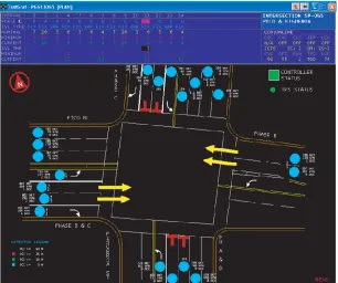
Figure 4-1 OASIS System Overview ... 82

Figure 4-2 NEMA Phase with Phase Sequence ... 83

Figure 4-3 Programmed Intersection Signal Phases ... 84

Figure 4-4 Dynamic Intersection Phases ... 85

Figure 4-5 Lead-Lag phase ... 86

Figure 4-6 Translink32 Data Download Schedule Display ... 87

Figure 4-7 Data Collecting Sites ... 88

Figure 4-8 Phase 2 g/C Profile for Timber Dr. Intersection ... 94

Figure 4-9 Phase 6 g/C Profile for Timber Dr. Intersection ... 94

Figure 4-10 Phase 2 g/C Profile for Jessup Dr. Intersection... 96

Figure 4-11 Phase 2 g/C Profile for Jessup Dr. Intersection... 96

Figure 4-12 Timber Dr Intersection Phase 2 Early Return to Green Distribution ... 98

Figure 4-13 Timber Dr Intersection Phase 6 Early Return to Green Distribution ... 98

Figure 4-14 Jessup Dr Intersection Phase 2 Early Return to Green Distribution ... 99

Figure 4-15 Jessup Dr Intersection Phase 6 Early Return to Green Distribution ... 100

Figure 4-16 Phase 1 and Phase 5 Displayed Green Distribution on Timber Dr. Intersection ... 101

Figure 4-17 Displayed Green Distribution on Jessup Dr. Intersection for AM Plan ... 102

Figure 4-18 Displayed Green Distribution on Jessup Dr. Intersection for PM Plan ... 103

Figure 4-19 AM Plan Outbound Programmed Bandwidth for Site “B” ... 105

Figure 4-20 AM Plan Inbound Programmed Bandwidth for Site “B”... 105

Figure 4-21 Dynamic Bandwidth for Site “B” ... 106

Figure 4-22 Dynamic Bandwidth for Site “A” ... 107

Figure 4-23 Dynamic Bandwidth Example ... 109

Figure 4-24 Split Monitor Example ... 110

Figure 4-25 DBAT Interface ... 113

Figure 4-26 DBAT Test Result of Alternate Progression Case ... 118

Figure 4-27 DBAT Test Result of Double Alternate System Case ... 120

Figure 4-28 DBAT Test Result of Simultaneous System Case ... 121

Figure 5-1 Example of Exhaustive Search Result ... 125

Figure 5-3 MAXBAND Optimal Solution (k>1) ... 134

Figure 5-4 MAXBAND Suboptimal Solution (k=1) ... 135

Figure 5-5 MAXBAND Suboptimal Solution (k=0.8) ... 135

Figure 5-6 Optimal solution from Propose LP (k=1)... 136

Figure 5-7 Optimal solution from Propose LP (k=0.8)... 137

Figure 5-8 LP Test Example 2 ... 139

Figure 5-9 “+” Operator Slack Analysis Result ... 141

Figure 5-10 “-” Operator Slack Analysis Result... 141

Figure 5-11 First Intersection Rear Slack Example ... 143

Figure 5-12 Dynamic Bandwidth LP Optimization Result... 146

Figure 5-13 Dynamic Bandwidth DBAT Exhaustive Search Result ... 147

Figure 5-14 Dynamic Bandwidth LP Optimization Result under Integer Constraints ... 149

Figure 5-15 LP and Exhaustive Search Method Solution (without Secondary Bands for Exhaustive Search Result and Integer Constraints on LP) ... 150

Figure 5-16 Exhaustive Search Result near Optimal Solution Area ... 151

Figure 5-17 Exhaustive Search Result Including Secondary Bands ... 152

Figure 6-1 US 70 Arterial in Clayton Primary Band with Secondary Band ... 157

Figure 6-2 Site “A” Outbound Bandwidth PDF and CDF ... 160

Figure 6-3 Site “A” Inbound Bandwidth PDF and CDF ... 160

Figure 6-4 Site “A” Day 1 AM Peak Plan Exhaustive Search Result ... 162

Figure 6-5 Site “B” Day 1 AM Peak Plan Exhaustive Search Result ... 163

Figure 6-6 Site “C” Day 1 AM Peak Plan Last 3 Intersection Exhaustive Search Result .... 164

Figure 6-7 DBAT Exhaustive Search Result in Plan 5 (Before) ... 168

Figure 6-8 Boxplot Result for Before and After Used Green Time ... 170

Figure 6-9 Coordinated Phase Used Green Time Comparison (Shotwell Dr. Intersection) . 171 Figure 6-10 Coordinated Phase Used Green Time Comparison (More St. Intersection) ... 172

Figure 6-11 Coordinated Phase Used Green Time Comparison (Robertson St. Intersection) ... 172

Figure 6-12 EB Before and After Travel Time CDF’s for 1:30 pm Plan at Site A ... 173

Figure 6-13 WB Before and After Travel Time CDF’s for 1:30 pm Plan at Site A ... 174

INTRODUCTION

CHAPTER 1

1.1 Background

According to the Texas Transportation Institute’s 2012 Annual Urban Mobility

Report, 1982 congestion costs were an estimated $24 billion (2011 dollars) resulting from 1.1 billion delay hours and 0.5 billion gallons of wasted fuel. The report further illustrates that these costs increased dramatically through 2011 when total congestion costs were an

estimated $124 billion resulting from 5.5 billion delay hours and 2.9 billion gallons of wasted fuel (Shrank 2007). Furthermore, the 2007 Traffic Signal Operation Self-Assessment Survey reported that Signal Operation in Coordinated Systems was given a “D-” grade, indicating that many signalized urban streets experience heavy congestion in the peak periods (National Traffic Signal Report Card 2007), and while the 2012 survey did not report a separate grade for operation in coordinated systems, the grade for Signal Timing Practices only improved from a “C-” to a “C” between the 2007 and 2012 surveys (National Traffic Signal Report Card 2012).

algorithms such as Optimized policies for Adaptive Control (OPAC) and Real-Time

Hierarchical Optimized Distributed and Effective System (RHODES) have emerged (Gartner 1983, Head et al. 1992). Also, the United Kingdom and Australia have developed Split Cycle Offset Optimized Technique (SCOOT) and Sydney Coordinated Adaptive Traffic System (SCATS) (Hunt et al. 1981, Lowrie et al. 1992). The objective of developing these

algorithms and systems is to help signals operate more efficiently.

However, there are several realistic limits to implementing adaptive signal control. Adaptive signal control operations require deploying several detectors to collect movement-specific traffic data. From that data, parameters are generated which require calibration by each system to estimate individual vehicle movements (travel time). Therefore, adaptive control systems typically require more installation and maintenance cost compared to traditional signal systems such as a closed loop system. In addition, it is necessary to train traffic signal engineers to operate adaptive systems which require extensive amounts of time and money.

One of the most common types of signal systems is the closed loop system which is a distributed traffic control system. This system consists of three components: the local

information for improving signal operation), still the offsets have to be entered into the system.

Well-designed signal coordination along arterial streets minimizes the number of stops and, consequently, travel delay. Synchronizing the onset of green indication for the intersections along an arterial street is one of the key steps in improving coordination and is known as offset optimization. Several studies, as will be discussed in the literature review section below, have addressed offset optimization assuming fixed-time signal-timing parameters. However, coordinated phase green times at intersections of an arterial under actuated control have dynamic rather than static durations. This is true because semi-actuated control allocates green time to non-coordinated phases only as needed based on detector calls, thereby reserving any unused green from non-coordinated phases for

additional green time for the coordinated movements. In other words, the controller can skip or terminate specific non-coordinated phases based on demand and allocate the unused green time to the major street coordinated movements. This phenomenon in semi-actuated,

coordinated control is called “early return to green”. Also, if all side-streets and major street left turn phases are skipped, then the major street green will be extended throughout the cycle. Therefore, since the duration of the coordinated phase green indication is dynamic, the resulting coordinated bandwidth is also dynamic, varying from cycle to cycle.

In addition, each intersection’s early return to green and green extension is independent of upstream and down-stream intersections, depending only on the local

analyzed by observing cycle by cycle phase durations. These characteristics of semi-actuated signal control make the coordination of signals along an arterial a challenging task if

dynamic bandwidth is to be taken into consideration.

However, this challenge brings the opportunity of improved understanding and improved arterial coordination. Analysis of dynamic bandwidth for current timing plans can provide valuable information to signal system managers and operators by assessing the impact of dynamic, coordinated phase green on dynamic arterial bandwidth. Furthermore, methodologies to optimize offsets along semi-actuated arterials based on observed phase durations hold the promise of improving signal coordination compared to optimization methods based on static programmed phase times. Improved arterial coordination will reduce traffic congestion, travel time, and the number of stops on arterial streets, thereby playing a role in addressing the chronic urban congestion problem highlighted above.

1.2 Problem Statement

Bandwidth is defined as the total amount of time per cycle available for vehicles to travel through a system of coordinated intersections at the progression speed, i.e. the time difference between the first and last hypothetical trajectory that can travel through the entire arterial at the progression speed without stopping.

coordination literature were conducted using programed (fixed) green times. However, most coordinated arterial signal systems operate in semi-actuated mode.

One approach to dealing with varying green time would be to use the observed average coordinated green durations. However, field studies show that the distribution of coordinated green times are typically asymmetrical. Therefore, using average green durations for developing a semi-actuated control strategy will not guarantee finding a near optimal set of offsets. In practice, signal engineers traditionally conduct field visits to observe the early return to green and the initial queue to fine tune the offsets and improve arterial performance based on engineering judgment.

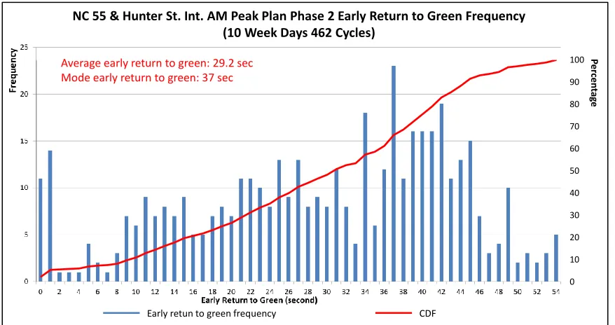
Figure 1-1 Intersection Early Return to Green Distribution

0 10 20 30 40 50 60 70 80 90 100

Early retun to green frequency CDF

P

er

cen

ta

ge

Average early return to green: 29.2 sec Mode early return to green: 37 sec

Figure 1-1 shows the frequency of early returns to green for an intersection on a coordinated system along NC 55 in Apex, NC. Only 2.38% of 462 cycles have no early return to green. The average additional green by cycle is 29.2 seconds with a primary mode of 37 seconds. It is also apparent from Figure 1-1 that the early return to green has a multi-modal distribution. The research to date on early return to green distribution has focused on using a fixed number to represent the distribution in the offset optimization process. The limitation of this approach is that a fixed value such as average, median, or mode cannot fully represent the entire early return to green given its characteristically asymmetrical, multi-modal distribution.

Furthermore, signal plan development traditionally relies on field manual fine-tuning. If the cycles observed during fine-tuning are not representative of normal conditions, this heavy reliance on limited observation fine-tuning could result in sub-optimal offsets. Finally, ongoing signal plan evaluation traditionally relies on costly field observations including before and after travel time runs. While this traditional approach can yield acceptable results, the process is time consuming, includes a relatively high degree of subjectivity, and by

necessity yields decisions that are founded on very a limited sample of operational conditions. In summary, no methodology currently exists to determine dynamic bandwidth on arterial streets using the signal operation data resident in deployed signal control systems, the primary surface street component of Advanced Transportation Management Systems

(ATMS). This study aims to bridge this gap by developing a methodology to determine dynamic bandwidths for semi-actuated coordinated arterial streets.

1.3 Objective

The primary objective of this study is to develop a methodology to determine

goal of continually improving signalized arterial performance. This research will focus on the following topics:

 Developing a dynamic bandwidth analysis algorithm and tool ;  Exploring the difference between traditional bandwidth and dynamic

bandwidth;

 Improving traditional bandwidth optimization method;

 Developing a new formulation for dynamic bandwidth optimization.

This research is expected to develop a dynamic bandwidth analysis algorithm and tool which can allow analysis of real bandwidth series from ATMS data sets and suggest feasible methodologies to find the global optimal offset point. Finally, this study will help to improve arterial performance, arterial signal management efficiency and give some important

information to traffic engineers that can support better engineering judgment.

1.4 Contribution

This thesis presents enhanced MAXBAND formulation is introduced to overcome the potential for the MAXBAND family of bandwidth optimization mixed-integer linear

function and constraints in the new formulation can be used to revise the formulations for all of the MAXBAND family of optimization models such as MULTIBAND, MULTIBAND-96, and AM-BAND.

In addition, this thesis presents a linear programming (LP) formulation to enable dynamic bandwidth maximization on semi-actuated arterial streets. The methodology relies on the use of archived signal log data regarding phase start and end times in each cycle in both directions. Those data are used to optimize the offsets that maximize the variable system bandwidth across multiple cycles constituting a coordination plan period. The formulation is also flexible to be used to optimize signal offsets using programmed (fixed) green durations at each intersection. The proposed formulation offers five significant enhancements

compared to traditional methods.

• The formulation is strictly linear (complexity of class P) as opposed to the traditional mixed integer programming formulations (complexity of class NP-hard).

• It can work with either static or dynamic (cycle varying) green durations. • Traditional bandwidth optimization methods have explicit constraints to

• The LP formulation enables the analyst to carry out a post-processing step which reports the range of offsets at non-critical intersections within which the optimal objective function value will be unaffected. This capability provides engineers with multiple solutions with identical bandwidths,

enabling the consideration of other performance measures such as stops, delay, or fuel consumption and emissions. The proposed formulation predicts the maximum proportion of traffic demand that can be served in the bandwidth, a unique attribute absent from other formulations found in the literature.

1.5 Organization

LITERATURE REVIEW

CHAPTER 2

For more than 100 years, traffic signals have served urban and suburban streets. Before traffic signals were developed, public officers such as policeman manually managed traffic movements. During past decades, many different computer based signal operation systems were developed for isolated intersection and coordinated arterials. This chapter reviews traditional offset optimization methods as well as various signal control system with arterial performance measures.

2.1 Signal System

2.1.1 Closed Loop System

1.a Open Loop System

1.b Closed Loop System

Figure 2-1 Open and Closed Loop System Process

Old forms of signal controllers are called electro-mechanical signal controllers, which are mainly composed of movable parts (cams, dials, and shafts) that control the passage of green, yellow and red lights in a predetermined sequence. Timings were controlled by mechanical tabs on a dial that were manually adjusted in the field by traffic engineers. These old systems do not provide any feedback loop in the system. They also do not allow

communication between the master signal and local signal controller. These old types of signal controllers are called “open loop systems”.

The closed-loop system is a distributed processor traffic-control system with control logic distributed among three levels (Traffic Signal Control System).

• The local controller

These systems provide two-way communication between the local controllers, on-street master, and between the on-on-street master and the office computer. Typically, the local controller receives information from field detectors. The master controller receives

information such as the status, time, and traffic volume from the local controllers. The office computer enables the system operator to monitor and control the system’s operations.

Three control modes are typically found with most closed-loop systems (Traffic Signal Control System).

• Manual mode • Time of day mode • Traffic responsive mode.

Under the Manual Mode, the operator specifies the pattern number of the desired traffic-signal timing plans and sequence via computer console. The time of day mode allows the controller unit to automatically select and implement a predetermined traffic-signal timing plan such as cycle, offset and split based on the time of day. With the traffic responsive mode, the computer automatically selects the predefined traffic-signal timing plan. This is the best fit to accommodate the current traffic flow conditions in the signal network. The pattern selection and implementation is accomplished through a traffic flow data matching technique executed every five minutes.

still widely used in CBD areas or similar environments where demand is over capacity. This type of controller provides exactly the same amount of green time to phases during each cycle. Fully actuated control is most often applied to non-coordinated signal controllers at isolated intersections. All phases are actuated so that the green duration of each phases is decided by minimum and maximum green and passage time, and, if necessary, pedestrian phase settings. Each phase can be extended, gapped out, or even skipped depending on demand and system settings. Therefore, in fully-actuated control there is no fixed cycle length. Volume-density represents the most complex legacy implementation of fully-actuated control with variable initial green based on arrivals on red and passage (gap) time that is shortened during the phase extension.

In semi-actuated signal control, only non-coordinated phases are actuated. All of the unused green time for non-coordinated phases reverts to the coordinated phases. This signal control scheme guarantees a programmed bandwidth (minimum bandwidth) for coordinated movements. Fully-actuated coordinated systems are similar to semi-actuated signal

controllers. They can allocate a portion of coordinated phases to non-coordinated phases. This means a portion of the coordinated phases are actuated (Day et al 2008).

A closed loop system coordinated system consists of six main components. • System detectors

• Local control equipment

• Controller master communications • On street master

• Office computer.

Among each component, the office computer allows the operator (traffic engineer) to set the time and date, display intersection, modify the master database, modify controller and coordination settings, modify system parameters, and monitor the system.

2.1.2 Traffic Responsive System and Adaptive Traffic Control System

Traffic responsive systems manage local controllers by updating cycles, offsets, and splits based on network level sensing. For example, traffic responsive plan selection (TRPS) involve matching defined plans to current traffic levels with this evaluation and selection normally taking place either in a field master controller or a central computer (Traffic Signal Timing Manual 2013). When the master or computer selects a new timing plan due to demand changes, it sends a command to all local signal controllers in a coordinated group instructing them to change to the new plan simultaneously. The master or central computer monitors multiple traffic condition data from an array of detectors, including data such as volume and occupancy. The detector data is processed to calculate values for a few key parameters that are compared to predetermined thresholds. When the thresholds are crossed, the most applicable timing plans from within the predetermined plans is implemented for the conditions represented by the threshold categories selected.

intersections to serve the predicted traffic flows. The signal controller utilizes prediction algorithms to compute optimal signal timings based on detected traffic volume and simultaneously implement the timings in real-time.

Miller introduced the principle of adaptive control for an online traffic modeling strategy (Miller 1963). The model calculates time wins and losses and combines these criteria for the different stages in the performance measures to be optimized. The first adaptive control system (PLIDENT), was implemented in Glasgow, United Kingdom (UK) in the 1960s. However, the system did not operated effectively. (Holroyd and Hillier 1971). The second adaptive control system field trial was in Canada (Corporation of Metropolitan Toronto 1976), but that trial also failed due to an inaccurate demand prediction algorithm for a longer time period, slowing the reaction of transition programs.

In the 1967, US Federal Highway Administration (FHWA) launched the Urban Traffic Control System (UTCS) project (Macgowan and Fullerton 1979). The stated objectives of the UTCS projects were (Stockfish 1984):

• To develop and test, in the real world, new computer based control strategies that would improve traffic flow.

The UTCS project identified three generations of adaptive control systems and the plan was to demonstrate and evaluate each generation of controls. The three generations are (Stockfish 1984):

• The first generation (UTCS-1) uses a library of predetermined timing plan, each developed with off-line optimization programs. The plan selected can be based on time of day, measured traffic pattern, or operator specification. The update period is 15 minute intervals. First generation allows critical

intersection control and has a bus priority system (Raus 1975, Macgowan and Fullerton 1979).

• The second generation (UTCS-2) uses timing plans computed in real time, based on predicted traffic conditions, using detector observations input into a prediction algorithm.

• The third generation was conceived as a highly responsive control with a much shorter control period than second generation and without the restriction of a cycle based system. Third generation system included a queue

Table 2.1. Comparison of Key Features of Three Generation of Control System

Feature First Generation Second Generation Third Generation

Optimization Frequency of

Update

Off-line 15 minutes On-line 5 minutes On-line 3-6 minutes

No. of Timing

Pattern Up to 40 Unlimited Unlimited

Traffic Prediction Critical Intersection

Control

No Adjusts split Adjusts split and offset Adjusts split, offset and cycle

Hierarchies of

Control Pattern selection Pattern computation

Congested and medium flow

Fixed Cycle Length Within each section Within variable groups

of intersection No fixed cycle length Source: Traffic Engineering (Mcshane et al. 1990)

(1984). In May of 1985, The UTCS project concluded and the policy statements were distributed on the support for the UTCS-1.5. The UTCS policy statement indicated that FHWA would not further enhance the software or documentation and that the private sector will likely develop and maintain their own system.

NCHRP 403 describes readily available adaptive control systems (NCHRP 403 2010). Several adaptive traffic control systems (ATCS) are currently deployed in the United States.

• Sydney Coordinated Adaptive Traffic System (SCATS) • Split, Cycle, Offset Optimization Technique (SCOOT) • Automatic Traffic Surveillance and Control (ATSAC) • Optimized Policies for Adaptive Control (OPAC)

• Real-Time Hierarchical Optimization Distributed Effective System (RHODES) • Adaptive Control Software-Lite (ACS-Lite)

• InSync

2.1.2.1 SCATS

In the late 1970s, the Road and Traffic Authority in New South Wales, Australia developed SCATS (Sims et al 1980). SCATS generate cycles, offsets and splits in three separate heuristic processes using calculated Degrees of Saturation (DSs) and link flows (LFs) from detector data (Lowrie , 1982, Stevanovic et al. 2009). Cycle length generated depends on two scenarios called low volume scenarios and high volume scenarios. Under the low volume scenarios, cycle length is determined from LFs. The high volume scenarios provided cycle length is computed using DSs. SCATS does not use common cycle lengths for

progression and selectively joins together intersections that have good progression. For offset adjustments, SCATS uses a number of predetermined offset plans and seeks the best offset for particular flow patterns. However, SCATS uses only stop bar detectors, so it cannot create real-time volume (demand) profiles. On the other hand, SCATS’ offset would not be sensitive against volume (demand) fluctuation.

2.1.2.2 SCOOT

Figure 2-2 SCOOT Operation Diagram

Source: http://www.scoot-utc.com/DetailedHowSCOOTWorks.php

2.1.2.3 ATSAC

ATSAC was developed by Los Angeles Department of Transportation (LA DOT). ATSAC does not have any formal optimization logic (algorithms) for adjusting signal timing. It instead applies heuristic formulas based on extensive systems operation experience (Rowe 1991). The adaptive adjustment of signal timings are based on second-by-second fluctuation of volumes and occupancies measured at system detectors. Cycle lengths are adaptively updated within predetermined upper and low boundaries. For a given system, splits are adjusted under minimum green time consideration after the current cycle length is set. ATSAC does not provide alternate phase sequences.

2.1.2.4 OPAC

The Optimized Policies for Adaptive Control (OPAC) strategy utilizes a real-time signal timing optimization algorithm developed at the University of Massachusetts at Lowell (Gartner 2001). OPAC is a fully-adaptive, proactive, and distributed real time traffic control system. The system was developed as part of the FHWA Real-Time Traffic Adaptive Control System (RT-TRACS) program (Andrews and Elahi 1997). The fundamental features of OPAC system are:

• Optimization of any or all phases splits designed to minimize total intersection delay and/or stops

• Support for phase skipping in the absence of demand

• Multiple sets of configuration parameters for customizing the resulting timing to weight certain movements for special circumstance or by time of day • Configurable to respond to changes in left turn lead/lag phasing by time of

day

• Special considerations for phase timing in the presence of congestion

2.1.2.5 RHODES

In 1992, the Real-Time Hierarchical Optimization Distributed Effective System (RHODES) was developed by the University of Arizona (Mirchanani and Head 2001). RHODES is a real-time traffic adaptive control system. It has a three-level hierarchical structure for characterizing and managing traffic and predicts traffic at these levels utilizing detector and other sensor information (Head et al. 1992). RHODES can receive and consider input from different types of detectors. Based on predicted future traffic conditions,

RHODES generates optimized signal control plans. Figure 2-4 illustrates the hierarchy of the RHODES system.

RHODES uses a dynamic programming (DP) based real-time signal control systems similar to OPAC. However, RHODES uses signal phases as stages, the amount of green-time as decision variables, and the total number of time-steps as state variables. The RHODES DP formulation requires a fixed sequence of phases and a longer forecast horizon. Since the RHODES DP formulation requires a fixed sequence of phases, it cannot optimize phase sequences. RHODES uses the REALBAND algorithm for its signal coordination (Dell’Olmo and Mirchandani 1995). REALBAND constructs a decision tree which contains all the possible decisions from the identified conflict movements. Each path in the decision tree represents a set of conflict resolutions that can be made within the system. The system calculates each path's performance such as delay and uses the calculated performance with path combination as constraints in the optimization algorithm.

2.1.2.6 ACS-Lite

ACS-Lite provides adaptive control within the industry standard context of cycle, splits, and offsets utilizing three control algorithms. Figure 2-5 shows that how the algorithms work in tandem to update traffic signal timing.

Figure 2-5 ACS-Lite Architecture (31)

2.1.2.7 InSync

The InSync system is an adaptive traffic signal system developed by Rhythm Engineering that uses advanced sensor technology, image processing, and artificial

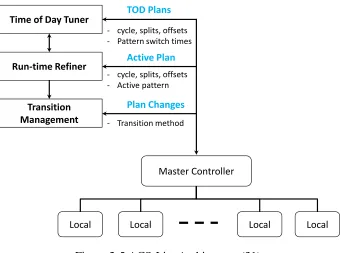
intelligence. The system uses a fundamentally different system of controlling and optimizing Time of Day Tuner

Run-time Refiner

Transition Management

Master Controller

Local Local Local Local

TOD Plans

- cycle, splits, offsets - Pattern switch times

- cycle, splits, offsets - Active pattern

- Transition method

Active Plan

signal phases and timings in real-time (no cycle length and phase sequence). InSync signal timing methodology includes three major components (NCHRP 403, 2010).

• Digital architecture • Global optimization • Local optimization

The “digital architecture” term refers to the concept of a “finite state machine”. In other words, InSync considers all possible non-conflict movement pairs and creates a maximum of “x” possible sequences of phase pairs at all intersections. Through the finite state machine framework, the InSync system can call any non-conflicting movement pair at any time. Thus, there is no predetermined phase sequence. The controller transitions signal indications from one state to the next based on the InSync logic, encapsulated by the local and global optimization algorithms.

This local and global optimization framework defines a two level optimization process. For global optimization, the InSync system focuses on time dependent platoon movements. The global optimizer in the system works to group platoons and optimizes their progression by maximizes the likelihood that each intersection’s coordinated phase will be green at that time each “time tunnel” (which has similar concept to “green band”) reaches the intersection. Conventional arterial coordination requires plan-based system cycle lengths for all coordinated signals. However, Insync does not require common cycle length for

time tunnels, each intersection runs its own local optimization (i.e. the “local optimizer”). The local optimizer allows each signal in the arterial to operate in an intelligent, fully actuated mode.

2.2 Performance Monitoring System

2.2.1 SMART-SIGNAL

In 2007, the University of Minnesota developed the Systematic Monitoring of Arterial Road Traffic and Signals (SMART-SIGNAL) system for monitoring arterial signal operation performance (Sharma et al. 2006, Sharma et al. 2008). Figure 2-6 shows overall architecture of SMART-SIGNAL.

The SMART-SIGNAL system collects two kinds of event signal data from “DATA Collection System”, which are vehicle actuation events and signal phase change events. Collected high resolution vehicle events data are used for estimating turning movement percentages and queue length. The results of dynamic queue length estimation and signal status date are processed for measuring each intersection's performance. Furthermore, the system generates “virtual prove car” to estimate arterial travel time to measure arterial performance.

2.2.1.1 Data Collection System

General actuated signal control systems are operated by detector call and the

operation results are displayed as signal phases. SMART-SIGNAL archives these two event data which are vehicle actuation events and signal phase change events. Those data sets are acquired separately from the data collection unit located in the traffic signal cabinet.

Traffic Event Recorder software program. The processed data is archived in Traffic Log Data Server.

Figure 2-7 Traffic Data Collection Flow in SMART-SIGNAL (Balke et al. 2005)

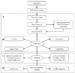
2.2.1.2 Data Processing

The archived raw data is processed and converted to an easy to read format for measuring intersection and arterial performance. The data processing procedure provides high resolution detector actuation data (second-by-second) such as volume and occupancy. It also provides cycle-by-cycle signal timing with status data, indicating each phases green start and end time. Figure 2-8 shows the SMART-SIGNAL data processing flow chart. The data process begins after the raw data is transmitted back to server. The data processing flow includes four steps.

• Preprocessing module

• Performance measure calculation • Visualization

The data verification step tests the collected data quality and filters out wrong data. The preprocessing module generates some basic measures from the raw data. The

performance measure calculation creates aggregated volume, delay, queue size, queue length, travel time etc. Finally the visualization step shows the results of different types of

performance measures and diagnosis' fine tuning of traffics signal system.

2.2.1.3 Intersection Performance Measurement

Many adaptive control systems use intersection delay and level of service as

intersection performance measurements. In the SMART-SIGNAL system, queue length and turning movement proportions (TMP) are used for measuring intersection performance.

For the queue estimation, SMART-SIGNAL uses a dynamic queue length estimation method. The model calculates difference of the arrival and departure rate and provides a queue length over time. The SMART-SIGNAL queuing model defines a number of event times that describe the dynamics of queue interaction with the signal status. The queuing model includes two separate estimation models which include “Short Queue Estimation Model” and “Long Queue Estimation Model”. If vehicle arrivals can be measured from advance detectors and queue length is less than distance between stop line and detector location, it is defined as “short queue”. Otherwise, it is defined as “long queue”. Short queue can be estimated according to the queue development using advance detector calls, which can provide vehicle headway. When queue spills over the advance detector, the advance detector will be occupied by a car and it will provide hi-occupancy. SMART-SIGNAL developed the relationship of queue development and occupancy profile at a signalized intersection. Using that relationship, maximum queue length and time-dependent queue length curve are

estimated. SMART-SIGNAL’s queue estimation procedure was compared to field data for 70 samples and was able to predict actual queue lengths with an average error of 7.5%, and queue sizes with an error of approximately 9.4%.

difficult to measure directly from detector calls since full-set detector configuration is rare in the field. Right-turn detectors are usually not deployed because a protect phase is absent at the majority of the intersections in the United States. Furthermore, shared lanes (through and right, or through and left) and exclusive left turn lanes with long loop detectors also make it difficult to measure turning movement proportions directly from detector calls.

SMART-SIGNAL proposed a simple turning movement proportion estimation model using advance detectors and left turn stop bar detectors for the major approach. Left-turn stop bar detectors were also used for the minor approach. Figure 2-9 shows SMART-SIGNAL detector configuration.

Figure 2-9 SMART-SIGNAL Detector Location Configuration (Balke et al. 2005)

2. The right-turn movement traffic in a cycle is continuous and uniform.

Based on two assumptions, SMART-SIGNAL estimates the short time intersection turning movement proportion. The suggested model was tested, a total of 56 sample cycles and 85 percentiles have errors of less than 15% and the average error was 8.9%. However, the error rate can vary site-by-site due to the second assumption.

2.2.1.4 Arterial Performance Monitoring Using Virtual Vehicle

SMART-SIGNAL uses a virtual probe vehicle to estimate time-dependent arterial travel time, utilizing high resolution vehicle actuation data and signal status data. The manually generated virtual prove vehicle has three possible maneuvers including acceleration, deceleration and no-speed-change.

Virtual probe decides its acceleration dependent on given traffic states, such as queue and signal status step-by-step. The step-by-step maneuver selection will be continued until its destination and the time different between start and end time will be an arterial travel time. Figure 2-10 shows step-by-step virtual prove maneuver decision tree.

The suggested model is tested on a 1.83 mile long major arterial on France Avenue in Minneapolis, MN. This arterial includes 11 signalized intersections with a coordinated actuation signal controller. Figure 2-11 shows the virtual probe vehicle’s trajectory with real floating car location. The study uses Root Mean Squared Percent Error (RMSP) as degree of model fitness. The reported estimation RMSP error is 0.0325, but the report did not mention test sample sizes.

2.2.2 Purdue Arterial Monitoring System (Day et al. 2010)

The Purdue Coordination Diagram (PCD) was developed by Purdue University and Indiana DOT. It uses phase status log and high resolution detector data for monitoring an intersection's level of performance and system level (arterial) performance. Figure 2-12 shows the Purdue monitoring systems flow.

Figure 2-12 Flowchart for Purdue Signal Monitoring System Source: NCHRP Project 3-79a

The Purdue system collects signal status data for monitoring cycle-by-cycle signal status. They developed a new analytical method to define dynamic cycle length. The created

Import data from Raw

Process Phase state change;

- Identify cycle boundaries - Measure cycle length

- Assign phase and cycle numbers

Count vehicles for each phase instance

Associate phase instance data (number of vehicles, green time) with cycles

Calculate intersection-level performance measures

dynamic cycle length and each phase will have a unique ID. In addition, each intersections detector high resolution data is also archived in the system for identifying vehicle arriving and vehicle location under the signal status. The Purdue signal monitoring system creates both intersection and arterial level performance measured by combining signal status data and high resolution detector data. Figure 2-13 shows controller log data sample.

The system log event data has three elements:

• A timestamp containing the data and time of the event, with resolution of 0.1 seconds.

• A number representing event type (Phase green, Phase yellow, Detector on, Detector off, etc.)

• A number representing the event channel. For phase information, this was the number of the phase for which the event was relevant.

2.2.2.1 Split Failure Monitoring

The Purdue monitoring system archives signal status log. The total green time for a phase in a defined cycle is found by summing over all instances of the phase that occur within cycle. Therefore, capacity can be estimated under assumed, observed or estimated saturation flow rates, such as the following equation.

𝐶_∅,𝑎 = 𝑔_∅,𝑎∗ 𝑆∅ 3600

Where, 𝐶∅,𝑎 : capacity provide to phase ∅ during cycle “a”

𝑔_∅,𝑎: the amount of effective green time for cycle “a” 𝑆∅ : saturation flow rate of phase ∅

The equation represents the total number of vehicles that can be expected to be served at the saturation flow rate. However, cycle lengths will be changed by time of day plan, so capacity per cycle in units of vehicles becomes difficult to compare between different cycle lengths. Therefore, the equation needs to be normalized as:

𝐶∅,𝑎 =

𝑔_∅,𝑎 𝐶𝑎 ∗ 𝑆∅

Where, 𝐶∅,𝑎 : capacity provide to phase ∅ during cycle “a”

𝑔_∅,𝑎: the amount of effective green time for cycle “a” 𝑆∅ : saturation flow rate of phase ∅

𝐶_𝑎 : cycle length of “a”

Figure 2-14 Observed Green Time Source: NCHRP Project 3-79a

High resolution detector data is archived in the system and provides a vehicle count during each cycle. The cycle-by-cycle vehicle counts are normalized by the following equation and it can be directly compared with estimated capacity.

𝑉_∅,𝑎= 3600𝑁∅,𝑎 𝐶_𝑎

Where, 𝑉_∅,𝑎 : hourly flow rate for phase ∅ during cycle “a”

𝑁∅,𝑎: the number of vehicle arriving during phase ∅ in cycle “a”

Combing the normalized hourly flow rate and capacity allows the degree of saturation or volume to capacity ratio.

𝑋_∅,𝑎= 𝑉∅,𝑎 𝐶_∅,𝑎

Where, 𝑋_∅,𝑎: normalized degree of saturation of phase ∅ during cycle “a” 𝑉_∅,𝑎 : hourly flow rate for phase ∅ during cycle “a”

𝐶∅,𝑎 : capacity provide to phase ∅ during cycle “a”

The degree of saturation gives a measure that quantifies how much the provided green time is utilized by vehicles. Figure 2-15 shows the volume to capacity ratio monitoring results. The number of dots above the red line indicates signal failure. This method allows monitoring the frequency of signal failure per time of day plan for each phase.

2.2.2.2 Purdue Coordination Diagram

The Purdue Coordination Diagram (PCD) is a visualization tool for evaluating the quality of progression. Figure 2-16 shows the result of high resolution detector data and phase status data for over several cycles. The green and orange lines indicate start and end time of green for each cycle. The black dots represent each vehicle's location. The PCD directly provides the arrival on green percentage for each cycle.

Figure 2-16 PCD over Several Cycles Source: NCHRP Project 3-79a

The black dots (vehicle location) are derived from advance detectors so the PCDs reflect actual vehicle behavior on the corridor. Figure 2-17 shows the 24 hour extended PCD. The PCD describes vehicle arrival with coordinated phase status, so this plot gives

Figure 2-17 PCD Over 24 hours Source: NCHRP Project 3-79a

2.3 State of Practice for Signal Timing Plan Development Process

The purpose of signal coordination is to provide smooth flow of traffic along streets and highways in order to reduce travel times, number of stops, and delays. A well-designed signal system allows platoons to travel along an arterial or throughout a network of major streets with minimum stops and delays. Designating traffic movement with the high peak hour demand as the coordinated phase is the most common practice to achieve these goals. The coordination logic (semi-actuated) reserves unused green time for the coordinated phase when non-coordinated phases have low demand. In general, this logic more stable capacity on coordinated phases and results in fewer stops for the high demand arterial traffic

movements.

Figure 2-18 Classical Approach to Signal Timing Source: NCHRP 409

arterial signal re-timing is decided to be necessary, the signal timing engineer conducts a travel time study to evaluating current conditions and progression quality. Many of DOTs in U.S. use the Tru-Traffic software for analyzing arterial travel time. Tru-Traffic allows the field travel time runs to be analyzed in relation to current timing plans. After conducting field travel time surveys, intersection turning movement data are collected. Computer based simulation and traffic analysis tools such as Synchro and Vistro are normally used for signal timing development. The collected turning movement counts for each intersection are essential input data for analysis and simulation. The computer analysis provides various signal timing options with an expected performance for each option. The signal timing engineer usually selects one of these near optimal timing plan options based on experience, expected performance, and engineering judgment for each of the time of day, day of week periods that will be served by a unique timing plan.

The next step is implementation of the selected signal timing plans in the field. After implementing the selected timing plan, the signal plan engineer conducts field fine-tuning of the coordination offsets. For the offset fine-tuning, the engineer visits the site to observe existing traffic conditions, paying special attention to operational characteristics such as each intersection’s initial queue length, early return to green, queue spill back, etc. The signal plan engineer must rely solely on experience and his/her engineering judgment for field offset fine-tuning. After completion of field fine-tuning, another travel time survey will be conducted for before and after comparison.

analysis tool can never provide an exact representation of the prevailing traffic conditions. In reality, many of the signal timing variables, such as minimum and maximum green time, green extension and etc., are given by or determined directly from policy. For example, NCDOT Traffic Management & Signal Systems Unit Design Manual provides guidelines for typical minimum green value (7 seconds), extension value (2 second for stretch detection, 3 seconds for low speed detection).

NCHRP 409 summarizes the current signal timing state of the practice by stating that: • Many agencies do not review field performance data to determine the

adequacy of signal timing at intervals less than three years.

• Many agencies do not review signal design, operations, maintenance, and training practices annually.

• Many agencies do not have precise and clearly stated policies that support detailed objectives.

2.4 Arterial Performance Measures

the intersections fit together in terms of signal timing. The performance measures include number of stops, travel speed, and bandwidth.

2.4.1 Number of Stops

The number of stops is used frequently to measure an arterial or network’s signal system effectiveness. Motor vehicle stops can often play a larger role than delay in the perception of the effectiveness of a signal timing plan a long an arterial street or a network. The number of stops or average numbers of stops per vehicle tends to be used more

frequently in arterial applications where progression between intersections is a desired objective. The number of stops has not been identified as a candidate for standardization nationally. In addition, this measure is difficult to collect directly on the field. Therefore, computer based simulation tools are normally used for estimating and optimizing the number of stops. Stops are highly correlated with amount of emission and the quality of progression along arterials. FHWA's Traffic Signal Timing Manual states that the number of stops is an important measure because acceleration from stops is a major source of vehicle pollutants and surveys reveal that multiple stops along an arterial is more highly correlated with driver frustration than is delay.

2.4.2 Travel Speed

HCM defines arterial LOS as a function of the class of arterial under the study and the travel speed along the arterial. This speed is based on intersection spacing, the running time

between intersections, and the control delay to through vehicles at each signalized intersection. Since arterial travel time (space mean speed) in HCM method is calculated segment by segment regardless of origin or destination, the resulting speed estimates may be different corresponding to speed (travel time) measurements made from end to end travel time runs. Data was collected by a GPS enabled floating car that measured a small subset of the possible origin-destination combinations along an arterial.

In HCM 2010, two performance measures are used to characterize LOS for a given direction of travel along an urban street segment. One measure is travel speed for through vehicles and the other measure is the volume-to-capacity ratio for the through movement at the downstream boundary intersection. Table 2.2shows the HCM 2010 level of service thresholds established for the automobile mode on urban streets.

Table 2.2 HCM 2010 LOS Criteria Travel Speed as a percentage of

Base Free Flow Speed (%)

LOS by Volume-to-Capacity Ratio

≤ 1.0 > 1.0

> 85 A F

> 67 – 85 B F

> 50 -67 C F

> 40 – 50 D F

> 30 – 40 E F

2.4.3 Bandwidth

The Federal Highway Administration Traffic Signal Timing Manual defines Bandwidth as the total amount of time available per cycle for vehicles to travel through a system of coordinated intersections at the progression speed, i.e. the time difference between the first and last hypothetical trajectory that can travel through the entire arterial at the progression speed without stopping. Bandwidth is an outcome of the signal timing that is determined by the offsets between intersections and the allotted green time for the

coordinated phase at each intersection. Bandwidth is a parameter that is commonly used to describe capacity or maximized vehicle throughput. Bandwidth can be confirmed by the time-space diagram which is visual toll for engineers to analyze a coordination strategy and modify timing plans. Bandwidth, along with its associated measures of efficiency and attainability, are measures that are sometimes used to assess the effectiveness of a coordinated signal timing plan.

Bandwidth efficiency is calculated by:

𝐵_𝑒 =(𝐵𝑊1+ 𝐵𝑊2) 2𝐶

Where, B_e: Two-way bandwidth efficiency 𝐵𝑊1: Outbound bandwidth

𝐵𝑊2: Inbound Bandwidth

Bandwidth attainability is calculated by:

Where, B_a: Two-way bandwidth attainability

𝑔𝑚𝑖𝑛1: Outbound direction minimum green along the arterial

𝑔_{𝑚𝑖𝑛2}: Inbound direction minimum green along the arterial

Table 2.3 and Table 2.4 show the FHWA Traffic Signal Timing Manual’s two Guidelines for bandwidth efficiency and bandwidth attainability.

Table 2.3 Guidelines for Bandwidth Efficiency

Efficiency Range Passer II Assessment

0.00 - 0.12 Poor Progression

0.13- 0.24 Fair Progression

0.25 – 0.36 Good Progression

0.37- 1.00 Great Progression

Table 2.4 Guidelines for Bandwidth Attainability

Attainability Range Passer II Guidance

1.00 – 0.99 Increase minimum through phase

0.99 – 0.70 Fine-tuning needed

2.5 Bandwidth Optimization

There are two distinct approaches to arterial bandwidth optimization. The first

approach produces uniform bandwidths, while the second provides variable bandwidths. Two well-known software tools that implement the first approach are MAXBAND (Little et al. 1981) and PASSER II (Messer et al. 1973).

Messer et al. (5) developed Progression Analysis and Signal System Evaluation Routine (PASSER II) in 1973. PASSER II is a macroscopic deterministic optimization model. An iterative gradient search method is used to determine the phase sequence and cycle length and can provide the maximum two-way progression for a specified arterial signal system. Brook’s Interference Algorithm (Brooks 1965) and Little’s Optimized

Unequal Bandwidth Equations (Morgan and Little 1964) are used in PASSER II. In PASSER II, cycle length, phase sequences, and offset are the decision variables and the objective is to minimize the total interference to progression.

Morgan and Little (1964) introduced a computation method to maximize arterial signal bandwidth. The widely used program of Little et al. (1966) efficiently finds offsets for maximum bandwidth given cycle time, red times, intersection spacing, and progression speed. Directional bandwidth weighting are set using a target value representing the directional flow rate ratio. Using a mixed-integer linear programming (MILP) approach, Little, Kelson and Gartner (1981) developed MAXBAND. The purpose of MAXBAND is to provide the maximum bandwidth setting for coordinated arterials. This program has the following capabilities:

• Allows for different progression speeds for each link within a given range • Provides optimal major street left turn phase sequencing

• Considers user specified queue clearance times

• Enables directional factors for two-way weighted bandwidth optimization

MAXBAND considers a two-way arterial with “n” intersections and specifies the corresponding offsets so as to maximize the number of vehicles that can travel within a given speed range without stopping throughout the arterial. Figure 2-19 shows the basic geometry defined for the MAXBAND mixed-integer linear program.

In MAXBAND, phase splits at each intersection are assigned according to Webster’s theory, and all signals are constrained to share a common cycle length. MAXBAND includes a queue clearance time in order to allow secondary flows which have accumulated during the red time to discharge before the platoon arrives.

The MILP form of MAXBAND is:

𝑀𝑎𝑥 𝑏 + 𝐾𝑏̅

subject to

{

𝑏̅ ≥ 𝐾𝑏 𝑖𝑓 𝐾 < 1 𝑏̅ ≤ 𝐾𝑏 𝑖𝑓 𝐾 > 1 𝑏̅ = 𝑏 𝑖𝑓 𝐾 = 1 }

𝑤𝑖+ 𝑏 ≤ 1 − 𝑟𝑖 ∀ 𝑖 = 1,2, ⋯ , 𝑛

𝑤̅_𝑖 + 𝑏̅ ≤ 1 − 𝑟̅_𝑖 ∀ 𝑖 = 1,2, ⋯ , 𝑛

(𝑡𝑖,𝑖+1+ 𝑡̅𝑖,𝑖+1) + (𝑤𝑖+ 𝑤̅𝑖) − (𝑤𝑖+1 + 𝑤̅𝑖+1) + (∆𝑖 − ∆𝑖+1) =

−1₂∗ (𝑟𝑖+ 𝑟̅𝑖) +1₂∗ (𝑟𝑖+1+ 𝑟̅𝑖+1) + (𝜏̅𝑖 + 𝜏̅𝑖+1) + 𝑚𝑖,𝑖+1 ∀ 𝑖 = 1,2, ⋯ , 𝑛

∆𝑖= (1₂) [(2𝛿𝑖 − 1)𝑙𝑖 − (2𝛿̅𝑖− 1)𝑙̅𝑖

𝑚𝑖,𝑖+1 = 𝑖𝑛𝑡𝑒𝑔𝑒𝑟 ∀ 𝑖 = 1,2, ⋯ , 𝑛 − 1

𝑏, 𝑏̅, 𝑤_𝑖, 𝑤̅_𝑖 > 0 ∀ 𝑖 = 1,2, ⋯ , 𝑛

𝛿_𝑖(𝛿̅_𝑖) = 𝑏𝑖𝑛𝑎𝑟𝑦

Where, 𝑏(𝑏̅) = 𝑜𝑢𝑡𝑏𝑜𝑢𝑛𝑑 (𝑖𝑛𝑏𝑜𝑢𝑛𝑑)𝑏𝑎𝑛𝑑𝑤𝑖𝑑𝑡ℎ; 𝐾 = 𝑡𝑎𝑟𝑔𝑒𝑡 𝑣𝑎𝑙𝑢𝑒 (𝑏̅_𝑏);