ABSTRACT
JUNG, YONG, Evolutionary Algorithm based Pilot Point Methods for Subsurface Characterization. (Under the direction of G. Mahinthakumar and S. Ranji Ranjithan).
Contaminated groundwater sites requiring remediation treatment exist all over the world. However, many of these sites have inadequate hydraulic information leading to inefficient cleanup strategies. Thus, many studies investigate the best way to obtain accurate hydraulic information (i.e., hydraulic conductivity or permeability) of the subsurface from secondary measurements such as hydraulic head and tracer/contaminant concentrations. Due to the limited amount of information and their associated uncertainty, these problems are often ill posed and non-unique. To minimize these shortcomings, different methods have been applied. An increasingly popular method to determine hydraulic conductivities in a given site is the pilot point method (PPM). The physical meaning of pilot points is that they are not direct measurement points; rather these selected points are added to the parameter search procedure to reduce the ill-posedness.
Two different evolutionary search based PPM approaches are developed in thesis as follows: 1) D-optimality sensitivity based method (SBM) that uses D-optimality criterion to search for pilot points and then a subsequent search for hydraulic conductivity values at these points, 2) A simultaneous search-based method (SSBM), where pilot points and hydraulic conductivities are searched simultaneously. These methods are first tested with hydraulic head measurements and then with both hydraulic head and concentration measurements using several synthetic problem scenarios.
Evolutionary Algorithm based Pilot Point Methods for Subsurface Characterization
by Yong Jung
A dissertation submitted to the Graduate Faculty of North Carolina State University
in partial fulfillment of the requirements for the Degree of
Doctor of Philosophy
Civil Engineering
Raleigh, North Carolina 2008
APPROVED BY:
DEDICATION
BIOGRAPHY
ACKNOWLEDGEMENTS
I would like to appreciate Dr. G. Mahinthakumar for all his endeavors to guide me and mentor me with wonderful insight. I would not forget his caring of my family during the study. I would like to thank Dr Ranji Ranjithan for his profound academic advice and continuous encouragements, and specially thank to Dr. Sankar Arumugam, and Dr. Sujit Ghosh for their time and effort as committees.
I would like to thank to the officemates, Matthew Clayton, Emily Zechman, Li Liu, Baha Mirghani, Michael Tryby, Kyutae Lee, Jitendra Kumar, and Xin Jin for their collaborations and encouragements.
I am truly indebted to my lovely parents (Dangchae Jung, and Yanglim Choi), parent-in-laws (Shinhan Bae, and Hwaja Tae), brother’s family (Kwon Jung, Hyunyoung Park, Gyum, and Sol) and sister’s family (Hairang Jung, Youngju Park, Yubin, Yudam, and Yuha), sister-in-laws (Kichung Bae and Juyoung Bae) for their true support and prayers.
Finally I truly present my love to my adorable God’s gift, MIN JUNG.
TABLE OF CONTENTS
LIST OF TABLES ...vii
LIST OF FIGURES...viii
Chapter 1: Introduction ...1
Chapter 2: Development and application of a Sensitivity based Pilot Point Method (SBM) for subsurface characterization...3
2.1 Introduction...3
2.1.1 Pilot points...5
2.1.2 Hydraulic conductivity estimation...7
2.2 Background ...8
2.2.1 Genetic Algorithm (GA) ...8
2.2.2 Kriging ...9
2.2.3 Forward Flow Model ... 10
2.3 Pilot Point Methodology (PPM)... 11
2.3.1 Determination of pilot points ... 12
2.3.2 Determination of hydraulic conductivity values ... 15
2.4 Test Problem and Results... 17
2.4.1 Synthetic Model... 17
2.4.2 Pilot point locations ... 21
2.4.3 Values at pilot point locations ... 25
2.4.4 Comparison with sequential search method... 28
2.5 Conclusion ... 30
2.6 References... 32
Chapter 3: Development of a simultaneous search based pilot point method (SSBM) and its comparison with the sensitivity based pilot point method (SBM) ... 37
3.1 Introduction... 37
3.2 Methodology ... 41
3.2.1 Simulation-Optimization Model... 41
3.2.2 Simultaneous Search-Based Method (SSBM) ... 43
3.3 Numerical Experiments ... 44
3.3.1 Scenarios ... 45
3.3.2 Objective and Penalty ... 47
3.4 Results... 48
3.4.1 SSBM and RANDOM ... 48
3.4.2 SSBM and SBM ... 53
3.5 Summary and Final Remarks... 56
3.6 References... 57
Chapter 4: Extension of SBM and SSBM to use both hydraulic head and tracer measurements ... 61
4.1 Introduction... 61
4.2.2 Max/Minimization Algorithm ... 66
4.3 Calibration: Sensitivity Based Method (SBM) ... 67
4.3.1 Overview of SBM... 67
4.3.2 Objective Functions ... 68
4.4 Numerical Examples of SBM ... 71
4.4.1 Hypothetical Models... 71
4.4.2 Different Scenarios ... 74
4.4.3 Numerical Comparison ... 75
4.5 Results and Discussions... 75
4.6 Conclusion ... 85
4.7 References... 87
LIST OF TABLES
<Table 2.1> Chosen genetic algorithm options in MATLAB... 21
<Table 2.2> D-optimality values of final selected pilot point locations for SBM ... 22
<Table 2.3> Head error values with sequentially selected points ... 29
LIST OF FIGURES
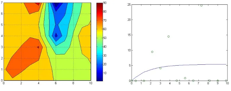
<Figure 2.1> Synthetic kriging results for this study (Left: semi-variogram graph with sill and range (x-axis: distance, y-axis: semi-variogram), Right: 3-dimensional figure for kriged hydraulic conductivity values (x- and y- axes: grid points, z-axis: hydraulic conductivity values), orange color indicates higher hydraulic conductivity) ... 10
<Figure 2.2> Flowchart of the sensitivity based pilot point method ... 12
<Figure 2.3> Synthetic groundwater field (unknown reality field; square = known hydraulic conductivity locations, triangle = hydraulic head measurement locations) and unknown reality of K-field ... 18
<Figure 2.4> Mean uniform (Left) and mean non-uniform (Right) flow contours for homogeneous hydraulic conductivity condition with constant heads at upstream (20 m) and downstream (15 m) respectively... 19
<Figure 2.5> Initial K-field distributions for four scenarios... 20
<Figure 2.6> Final selections of pilot points in four scenarios ... 22
<Figure 2.7> Comparisons of D-optimality values between random pilot point sets and GA optimized pilot point sets... 23
<Figure 2.8> Sum of correlations (left axis) of pilot point locations and their sensitivity metric (right axis) from random and SBM... 24
<Figure 2.8> Sum of correlations (left axis) of pilot point locations and their sensitivity metric (right axis) from random and SBM. (Continued) ... 25
<Figure 2.9> Head error values from pilot point locations from D-optimality (Det-PPL) and sensitivities of randomly selected locations (Random) ... 26
<Figure 2.10> Contour maps of scenario_2 (Top left: unknown reality, Top right: initial contour, Bottom left: without penalty, Bottom right: with penalty)... 28
<Figure 2.11> Sequentially searched pilot point locations with the selection order and final hydraulic conductivity distribution (Using four selection) ... 29
<Figure 3.1> Simultaneous search based pilot point method... 44
<Figure 3.2> Hydraulic conductivity distribution of unknown reality ... 45
<Figure 3.3> Initial hydraulic conductivity distributions (From left top to right bottom: Scenario_1, Scenario_2, Scenario_3, and Scenaro_4)... 46
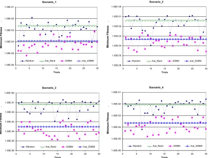
<Figure 3.4> Comparison of minimum fitness comparison from random locations and SSBM ... 50
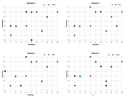
<Figure 3.5> Final pilot point locations using SSBM with measurement points of hydraulic conductivities and hydraulic heads for four different scenarios51
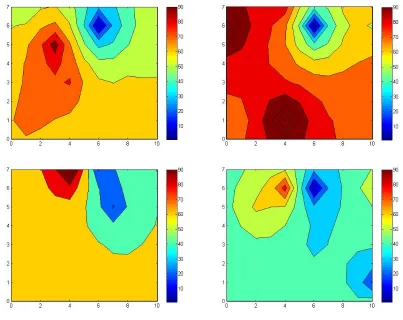
<Figure 3.6> Final hydraulic conductivity contour maps (From top left to right: Scenario_1, Scenario_2, Scenaro_3, and Scenario_4)... 52
<Figure 3.7> Average minimum fitness from thirty trials and average hydraulic conductivity difference... 54
<Figure 3.8> Contour maps of unknown reality, initial distribution of scenario 2 (Top left and Top right) and final distribution from SBM and SSBM respectively (Bottom left and bottom right) ... 55
<Figure 4.1> Flow chart of coupled inverse problems using SBM... 68
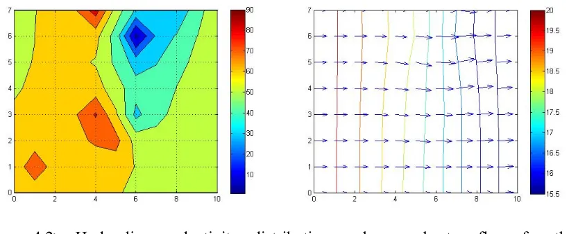
<Figure 4.2> Hydraulic conductivity distribution and groundwater flow for the unknown reality ... 72
<Figure 4.3> Initial tracer injection line with the transport depending on time in the domain (triangles: observation points, and dark line: Tracer injection points in initial injection domain)... 73
<Figure 4.4> Hydraulic conductivity measurement locations and initial hydraulic conductivity distributions based on kriged measurements for scenario 1 and 2 ... 74
<Figure 4.5> Comparison between various information based pilot point method using average of relative hydraulic conductivities and average of maximum hydraulic conductivity differences... 76
head/concentration observation locations, and circles: optimal pilot point locations) ... 77
<Figure 4.7> Combination of pilot point locations from head and concentration or quantile separately (In scenario 1, the combinations of head and concentration or head and quantile are located in the same points) ... 79
<Figure 4.8> Comparison between SBM and SSBM ... 81
<Figure 4.9> Final pilot point locations using SSBM ... 81
<Figure 4.10> Hydraulic conductivity distributions from SBM and SSBM for scenario 1 and 2 ... 82
<Figure 4.10> Hydraulic conductivity distributions from SBM and SSBM for scenario 1 and 2 (Continued) ... 83
Chapter 1:
Introduction
Chapter 2:
Development and application of a Sensitivity based Pilot
Point Method (SBM) for subsurface characterization
2.1Introduction
Inadequate representation of the hydraulic conductivity or permeability of the subsurface is one of the greatest sources of uncertainty in developing good groundwater flow and transport models for field applications. Unfortunately, very few direct hydraulic conductivity measurements are available for most sites. Given this reality, considerable research has been expended during the last few decades in developing methods that can improve hydraulic conductivity estimates from secondary measurements such as hydraulic head or tracer concentrations. These methods fall under the category of inverse modeling methods as hydraulic conductivity field is input to a groundwater flow and transport model while hydraulic heads and tracer concentrations are output. Given the potentially large parameter space and lack of adequate secondary measurements, combined with the uncertainties of prior information and simulation models, these inverse problems are generally ill-posed suffering from non-uniqueness, instability, and non-existence. A number of texts and publications including Yeh (1986), Carrera and Neuman (1986), Dietrich and Newsam (1990), and McLaughlin (1996) provide excellent reviews on this topic.
addition, regularization is employed to the objective function to further reduce non-uniqueness (Emsellem and de Marsily 1971, and Carrera and Neuman 1986a, 1986b). Regardless of the representation of the hydraulic conductivity field, both optimization based (i.e., nonlinear least squares) and geostatistical inversion based techniques can be used. Geostatistical inversion methods are based on a linearized relationship between the geostatistical models of the hydraulic conductivity with secondary measurements such as hydraulic heads (Gutjahr et al. 1978, Keidser and Rosbjerg 1991, and Sun and Yeh 1992). However, the linearization assumption used in these methods is often valid for small variances in the hydraulic conductivity field, which may not represent reality (Certes and de Marsily 1991, RamaRao et al. 1995, LaVenue et al. 1995, and Hendricks-Franssen 2000). Optimization based methods adjust the hydraulic conductivity field in a systematic fashion to match the secondary measurements by simulating these measurements using a forward groundwater flow or transport model. While these methods have a more general applicability, unless the parameter space is reduced by a proper representation of the hydraulic conductivity field, they can suffer from issues such as non-uniqueness and instability. Pilot point methods (PPM) offer a promising alternative to zonal models and improvement over traditional geostatistical models in reducing the parameter space in an optimization based inversion approach. This method was first proposed by De Marsily et al. (1984) where a set of calibration points called “pilot points” are selected from the model domain at which the hydraulic conductivity is adjusted to match the head measurements. A number of researchers have the modified the PPM and applied it to different situations in terms of reducing instability that results from over-parameterization and huge fluctuations of estimated parameter values (Fasanino et al. 1986, Certes et al. 1991, LaVenue et al. 1992, 1995, 2001, RamaRao et al. 1995, Oliver et al. 1996, Cooley 2000, Vesselinov et al. 2001a, 2001b, Medina et al. 2003, Hernandez et al. 2003, Doherty 2003, Kowalsky et al. 2004, Alcolea et al. 2005).
kriging) based on measured hydraulic conductivity values, 2) select pilot point locations where no values of measured hydraulic conductivity are available and use only kriged values, 3) iterate to find optimal values of hydraulic conductivity at selected pilot point locations by minimizing an objective function (generally, the sum of squared differences between observed hydraulic heads and calculated hydraulic heads obtained using a forward model) and krige hydraulic conductivity field, 4) a final hydraulic conductivity field will be obtained by previous iterations and kriging. Comparative studies for the PPM with other nonlinear inverse approaches can be found in Keidser and Rosbjerg 1991, McLaughlin et al. 1996, Zimmerman et al. 1998, Floris et al. 2001, Carrera et al. 2005. Following the given basic approach, we focus on the optimal number and location of pilot points to prevent over-parameterization and reduce instability.
2.1.1 Pilot points
Instead of using pilot point locations, Sahuquillo et al. (1992), Gomez-Hernanez et al. (1997), Capilla et al (1998), Hendricks Franssen et al. (1999), Wen et al. (1998a, 1998b, 1999, 2002) used master point locations to reduce the parameter space. The resulting method is known as the Sequential Self-Calibration (SSC) method. SSC is conceptually similar to PPM except the use of master points, which are randomly selected imaginary grid points and used as hydraulic conductivity perturbation locations. Master point locations, however, should fulfill the basic need of one-third variogram correlation range of hydraulic conductivity measurements. For this reason, only one or two master location(s) should be in the correlation range as the rule of thumb. For instance, Wen et al. (1998b) used the range of the hydraulic conductivity variogram and number of observation wells as criteria to decide the number of master locations and assign fewer master locations for fewer wells or wide-ranging correlation lengths. As in most previous studies, this study also uses the number of observation wells as a basic criterion for the determination of number of pilot point locations. However, their locations will be based on criteria that include both sensitivity and parameter correlation. This is different from sensitivity based methods used by LaVenue and Picken(1992), RamaRao et al (1995), and LaVenue et al (1995). The criteria will be discussed in detail in the methodology section (2.3).
2.1.2 Hydraulic conductivity estimation
applications of GA for hydraulic conductivity or permeability estimation in petroleum reservoir and groundwater domains (Sen et al. 1995, Bush et al. 1996, Guerreiro et al. 1998, Romero et al. 2000, Karpouzos et al. 2001, Romero et al. 2002). In this study we propose a GA based search approach for pilot point location selection as well as hydraulic conductivity estimation at the selected pilot points.
The remainder of this paper is organized as follows. The next section, Background, provides a description of the computational components, section 2.3 describes the pilot point method developed in this paper, including descriptions of genetic algorithm, geostatistics, groundwater flow model, and numerical experiment. Section 2.4 presents the test problem with results and discussion of application of the pilot point method, followed by Section 2.5, Conclusions.
2.2Background
The pilot point method developed in this paper uses three main computational components: (a) a genetic algorithm based search method for locating pilot points and determining hydraulic conductivity values, (b) simple kriging for interpolation of values, and, (c) a groundwater flow model for determining hydraulic head values from K-field. For simplicity, these computational components are implemented in a MATLAB environment.
2.2.1 Genetic Algorithm (GA)
selection, crossover, mutation, and elitism. In GA the decision variables are usually encoded as real or binary strings. In this paper, the decision variables are either the pilot point locations (integer node indices in the grid) or hydraulic conductivity values. For simplicity, real representation is used for these decision variables. The built-in genetic algorithm function in the MATLAB GA toolbox is used in this paper.
2.2.2 Kriging
Kriging/co-kriging is an interpolation tool to obtain unbiased predicted values of hydraulic conductivities over a set of grid points based on observed correlated values at certain points. Moreover, this has the advantage of reproducing smooth surface of optimal hydraulic conductivities from hydraulic conductivity perturbations at pilot point locations. In most applications, kriging is based on the assumption that the observed values are generated from an intrinsic stationary stochastic process defined over a space or region. Intrinsic stationarity implies that the mean of the process is constant and the variance of the difference of two response values depends only on the distance between the locations. More specifically, if Z(s) represents hydraulic conductivity at location s,
then
{
Z(s), s!D}
is said to be intrinsic stationary, if (i) E Z(s)[
]
=µ, !s"D and (ii)Var Z
[
(s1)!Z(s2)]
=2"(s1!s2), #s1,s2 $D.For this study, the exponential model (!(h)=c0+c1"(1#e#3||h||/a)) for semi-variogram is
applied where the sill, c1represents the maximum of semi-variogram of measured
hydraulic conductivity; range, a denotes thecorrelation distance of observations, beyond this distance observations are not correlated; and nugget, c0 represents micro scale
Kriging is reapplied using the perturbed and measured conductivity values to produce the final estimate of hydraulic conductivity values. Figure 2.1 shows the semi-variogram and hydraulic conductivity field from a given synthetic example for this study.
<Figure 2.1> Synthetic kriging results for this study (Left: semi-variogram graph with sill and range (x-axis: distance, y-axis: semi-variogram), Right: 3-dimensional figure for kriged hydraulic conductivity values (x- and y- axes: grid points, z-axis: hydraulic conductivity values), orange color indicates higher hydraulic conductivity)
2.2.3 Forward Flow Model
The forward groundwater flow model is based on a central difference approximation of the steady state groundwater flow equation:
( , ) h ( , ) h 0
T x y T x y
x x y y
! ! ! !
! ! ! !
" #
" #+ =
$ %
$ %
& ' & ' eq 2.1)
where
T(x,y) = Isotropic, heterogeneous, transmissivity field(k x y( , ) Aquifer depth! )
This forward model is used to obtain the head field h(x,y) for a given hydraulic conductivity field k(x,y).
2.3Pilot Point Methodology (PPM)
<Figure 2.2> Flowchart of the sensitivity based pilot point method
As shown in figure 2.2, the two separate procedures are sequentially carried out.
2.3.1 Determination of pilot points
The most sensitive locations with least correlation ought to be selected as pilot points, as this will maximize the data worth of the hydraulic head measurements. In other words, these would be the most unique set of points that require minimal perturbations of hydraulic conductivities to match hydraulic head observations. A criterion that satisfies these conditions is the D-optimality criterion mathematically expressed as (J. Kiefer and W. Keifer, 1959, Fedorov et al., 1968)
MAXIMIZE obj_1=det[XT
X(n!m) =
"h1
"k1
"h1
"k2
# # # "h1
"km
"h2
"k1
"h2
"k2
# # # "h2
"km
# # # # # #
# # # # # #
"hn
"k1
"hn
"k2
# # # "hn
"km
$ % & & & & & & & & & & & & & ' ( ) ) ) ) ) ) ) ) ) ) ) ) ) eq 2.3) where
obj_1: objective function in first procedure X: sensitivity matrix
h: hydraulic head observation (n-number of hydraulic head observations) k: hydraulic conductivity values at potential pilot point locations
(m-number of selected pilot points)
A key quantity in this procedure is the sensitivity matrix (X) shown in equation 2.3 that measures the sensitivity of hydraulic heads with respect to hydraulic conductivities at potential pilot point locations. As equation 2 shows, we are maximizing the determinant
of the Fisher information matrix (XTX), which is known as D-optimality. If A= XTX
and variance-covariance matrixB=A!1, the correlation matrix C is simply the covariance
changes. In other words, changes in hydraulic conductivity at any two points from this set will invoke dissimilar changes in head values at the head observation points. In an optimization sense, these set of points are less prone to non-uniqueness as we are more likely to find a unique set of hydraulic conductivity values at these points to match the head observations. As opposed to minimizing the determinant or norm of the covariance matrix, the D-optimality criterion (i.e., maximizing the determinant of the Fisher information matrix) has two additional advantages. First, it does not require calculation of the correlation matrix thus resulting in significant computational savings and smaller impact of round off errors. Second, D-optimality also ensures that the pilot points selected are highly sensitive to the head observations; a larger determinant value will ensure larger diagonal values (higher sensitivity) and smaller off diagonal values (lower correlation). Higher sensitivity means that smaller perturbations are required at the pilot points to match the head observations thus nearly preserving the original correlation structure of the measured hydraulic conductivities.
Similar to the D-optimality criterion, the sequential search method (SSM) employed by LaVenue et al. (1992) using adjoint sensitivity also ensures that the points selected are maximally sensitive. Since the points are selected one at a time, in terms of the scale of sensitivity, norm function (maximum of the matrix singular value decomposition) to get magnitude of the matrix elements is sufficient. However, unlike D-optimality, SSM does not ensure that the combined set of pilot points is least correlated as described earlier. Due to these advantages, D-optimality has been used for a number of applications including parameter estimation in groundwater (Knopman et al. 1987) and characterization of water distribution systems (Bush et al. 1998). To our knowledge, it has not been used in pilot point selection.
redundant pilot points and the matrix X will be rank deficient (number of unknowns m >
number of rows n). This would likely make the fisher information matrix (XTX) to be
linearly dependent forcing its determinant (D-optimality) to be essentially zero. A number m that is too small will not make efficient use of the observed head values. Based on these observations and preliminary tests conducted with different number of pilot points, in this study, we chose the number of pilot points to be one less than the total number of head measurements. Since the number of head measurements is always four in this study we fix the number of pilot points to three (see 4.2).
Heuristic unconstrained search optimization approaches such as GA’s frequently enforce constraints by the use of penalty functions. These are simply penalty values added to the objective function to encourage search towards a feasible space. Since the version of the MATLAB GA toolbox used in this paper did not support constraints, penalties were used to enforce constraints. In the pilot point location search procedure, bound constraints limiting the pilot points to nodes in the computational domain are enforced by adding a penalty whenever this is violated. The measurement locations were avoided in the search by encoding the decision variables (pilot point locations) by excluding the measurement locations. The D-optimality criterion automatically ensures that no two pilot points are the same since the value of D-optimality in this case would be zero.
2.3.2 Determination of hydraulic conductivity values
MINIMIZE obj_ 2=
"
(hobserved !hcalculated)2 eq 2.4)where
obj_2: objective function
hobserved: observed hydraulic head values
hcalculated: calculated hydraulic head values
Since hydraulic heads are primarily sensitive to spatial variations of hydraulic conductivity than their absolute magnitudes, it is customary to constrain the magnitude of hydraulic conductivity based on prior information to reduce the search space (e.g., LaVenue et al. 1992). In this paper, we use the geometric mean of measured hydraulic conductivity values to narrow down the hydraulic conductivity search space. To accomplish this, we add a penalty to the objective in equation 2.5 if the geometric mean of the hydraulic conductivity values at the pilot points (gp) deviates from the geometric mean of the measured hydraulic conductivity values (gm) by more than 75 %.
...
if
|
gm
!
gp
|
gm
>
0.75
obj
_ 2
=
obj
_ 2
+
|
gm
!
gp
|
gm
end
...
eq 2.5)
where
2.4Test Problem and Results
2.4.1 Synthetic Model
A 2-dimensional synthetic site (700 m by 1000 m) with regular shape of grid blocks (100 m by 100 m) shown in figure 2.3 is used for numerical tests. This synthetic groundwater flow field is based on a confined, isotropic, and heterogeneous aquifer exhibiting mean or non-mean uniform flow presented in figure 2.4. The flow field is obtained by applying constant head boundary conditions at the left (upstream) and right (downstream) boundaries (scenario 1 and 2) or left (upstream) and bottom (downstream) boundaries (scenario 3 and 4) and no-flow boundary conditions at the other sides. The upstream and downstream boundaries have 20 m and 15 m constant hydraulic heads respectively.
Flow 1 (Scenario 1 &2) Flow 2 (Scenario 3 & 4)
<Figure 2.4> Mean uniform (Left) and mean non-uniform (Right) flow contours for homogeneous hydraulic conductivity condition with constant heads at upstream (20 m) and downstream (15 m) respectively.
Field 1 (Scenario 1 & 3) Field 2 (Scenario 2 & 4)
<Figure 2.5> Initial K-field distributions for four scenarios
Re K Error= 1
Nt
(Kci !Kri)
2
i=1
Nt
"
eq 2.6)where
Nt: Total number of known hydraulic conductivity
Kci: Calculated hydraulic conductivity
Kri: True hydraulic conductivity
<Table 2.1> Chosen genetic algorithm options in MATLAB First Procedure
(Location Search)
Second Procedure (Value Search)
Population Double Vector Double Vector
Selection Tournament Stochastic uniform
Cross over Scattered (0.6) Scattered (0.4)
Mutation Uniform (0.3) Uniform (0.3)
Population Size 100 1000
Number of Generations 100 100
2.4.2 Pilot point locations
<Figure 2.6> Final selections of pilot points in four scenarios
The final D-optimality values for the pilot point sets from the GA search are presented in Table 2.2 for each scenario. One might notice that these values are extremely small. This is plausible as hydraulic heads are known to have very low sensitivities to the magnitude of hydraulic conductivities that are perturbed at the pilot points. However, hydraulic heads are sensitive to the variability of hydraulic conductivity that is exploited when the pilot points are selected in a collective fashion.
<Table 2.2> D-optimality values of final selected pilot point locations for SBM Scenario_1 Scenario_2 Scenario_3 Scenario_4
In order to evaluate the effectiveness of GA in searching pilot point locations with high D-optimality values, we calculated D-optimality values of thirty random pilot point sets (3 points in each set) in each scenario and compared it to the values obtained by the GA search. These are presented in figure 2.7. In the figure 2.7, squares represent the D-optimality value from GA search and the diamonds represent values for randomly selected pilot point locations. Clearly, for all four scenarios, the D-optimality values for the pilot points searched by GA are one or two orders of magnitude greater than those for a random set of pilot points. This indicates that GA is effective in searching for pilot points with high D-optimality values.
To evaluate the effectiveness of the D-optimality metric in SBM, two additional metrics are calculated: (1) Sum_corr = Sum of correlations between individual pilot point locations (sum of the absolute values of the off-diagonal entries of the correlation matrix described in section 3.1), (2) Norm_sens = Norm of sensitivity matrix. The Sum_corr metric measures the correlation among the selected set of pilot points. A low sum_corr value is better for estimation as this will minimize non-uniqueness. The norm_sens metric measures the sensitivity of the pilot points to the measured hydraulic heads. A high norm_sens metric is better for estimation as this will reduce the amount of perturbation required to match the measured head values. In Figure 2.8 we compare these metrics for SBM pilot points and random pilot points for the 4 scenarios for 30 random trials. In most cases, the pilot points from SBM are less correlated with significantly larger sensitivities. Occasionally randomly selected pilot point locations provide less correlated locations but with insignificant sensitivity values. In other cases, the random pilot point locations are highly sensitive to the hydraulic head measurements, but these locations are strongly correlated each other. In other words, the SBM based pilot points provide a good compromise between these two metrics.
<Figure 2.8> Sum of correlations (left axis) of pilot point locations and their sensitivity metric (right axis) from random and SBM. (Continued)
2.4.3 Values at pilot point locations
hydraulic conductivity distribution is significantly different from the unknown reality (scenario 2 and 4), SBM provide more accurate hydraulic conductivity estimation with minimum fluctuations. When comparing the cases with different flow conditions, mean non-uniform flow cases (scenarios 3 and 4) result in slightly larger fluctuations in hydraulic conductivity estimates and larger hydraulic head errors for both SBM and Random. Other than that, different flow conditions do not significantly influence hydraulic conductivity estimation for these problem sets. From these results, we can conclude that, in general, the D-optimality based pilot point selection is superior to random selection and is a viable and promising alternative to other methods of pilot point selection for various conditions.
<Figure 2.10> Contour maps of scenario_2 (Top left: unknown reality, Top right: initial contour, Bottom left: without penalty, Bottom right: with penalty)
2.4.4 Comparison with sequential search method
<Table 2.3> Head error values with sequentially selected points
No. X Y Hydraulic
Conductivity (K) Head error
Average error of actual Ks
1 9 4 49.245 0.112 1.881
2 9 2 61.857 0.112 1.896
3 1 4 84.744 0.104 2.002
4 10 4 71.586 0.092 2.010
<Figure 2.11> Sequentially searched pilot point locations with the selection order and final hydraulic conductivity distribution (Using four selection) (Continued)
2.5Conclusion
hydraulic conductivity search process. Furthermore, SBM is shown to perform much better than a previously developed sequential search method.
There are several limitations of this study that could be explored in the future:
• The impact of the accuracy of the sensitivity matrix X (equation 2.3) has not been examined. A major consideration in the accuracy is the size of denominator (!K) used in calculating the sensitivity matrix X. If the head response is nonlinear to changes in K values, the fixed !Kvalue of 1 is used in this study might not be appropriate if the perturbation of hydraulic conductivity values at the pilot points in the second step are of different magnitude.
• Comparison with another method such as simultaneously searching for pilot point locations and their hydraulic conductivity values to match the head measurements has not been pursued. This will be investigated in a subsequent paper.
• The effect of incorporating tracer concentration measurements in the pilot point selection and hydraulic conductivity estimation has not been studied. This will be investigated in a subsequent paper.
2.6References
Alcolea, Andres, Jesus Carrera, and Agustin Medina, Pilot points method incorporating prior information for solving the groundwater flow inverse problem, Advances in Water Resources, 2006.
Bush, M. D., J. N. Carter, Application of a modified genetic algorithm to parameter estimation in the petroleum industry, Intelligent Engineering Systems through Artificial neural Networks 6, ASME Press, 397, 1996.
Bush, Cheryl A., and James G. Uber, Sampling design methods for water distribution model calibation, J. of Water Resources Planning and Management, Vol. 124, No. 6, Nov/Dec 1998.
Capilla, Jose E., Jaime Gomez-Hernandez and Andres Sahuquillo, Stochastic simulation of transmissivity fields conditional to both transmissivity and piezometric data Demonstration on synthetic aquifer, J. of Hydrology, 203, 175-188, 1997.
Carrera, Jesus, and Shlomo P. Neuman, Estimation of aquifer parameters under transient and steady state conditions: Uniqueness, Stability, and Solution Algorithms, WRR, Vol. 22, No. 2, 211-227, 1986.
Carrera, Jesus, Andres Alcolea, Agustin Medina, Juan Hidalgo, and luit J. Sloothen, Inverse problem in hydrogeology, Hydrogeology J., 13, 206-222, 2005.
Certes, Catherine, and Ghislain de Marsily, Application of the pilot point method to the identification of aquifer transmissivities, Adv. Water Resources, Vol. 14, No. 5, 1991.
Chavent, G. and R. Bissell, Indicator for the refinement of parameterization, Inverse Problems in Engineering Mechanics, Int. Symposium on Inverse Problems in Engineering Mechanics, Japan, M. Tauaka and G.S. Dalikravich (Eds.), Elsevier Science, 1998.
Clifton, P. M., and S. P. Neuman, Effects of kriging and inverse modeling on conditional simulation of the Avra Valley aquifer in southern Arizona, WRR, Vol. 18, No. 4, 1212-1234, 1982.
Cooley, Richard L., An analysis of the pilot point methodology for automated calibration of an ensemble of conditionally simulated transmissivity fields, WRR, Vol. 36, No. 4, 1159-1163, April 2000.
de Marsily, G., De L’identification des systems hydrogeologiques, thesis, Univ. of Paris VI, 1978.
de Marsily, G., G. Lavedan, M. Boucher, G. Fasanino, Interpretation of interference tests in a well field using geostatistical techniques to fit the permeability distribution in a reservoir model, Geostatistics for natural resources characterization, pt.2, D. Reidel Publishing Company, 1984.
Dietrich, C. R., and G. N. Newsam, Sufficient conditions for identifying transmissivity in a confined aquifer, Inverse Problmes 6, L21-L28, 1990.
Doherty, John, Ground water model calibation using pilot points and regularization, Ground Water, Vol. 41, i.2, 170-178, Mar.-Apr. 2003.
Emsellem, Y., and G. de Marsily, An automated solution from the inverse problem, WRR, Vol. 7, No. 5, 1264-1283, 1971.
Fasanino, G., J.-E. Molinard, G. de Marsily, and V. Pelce, Inverse modeling in gas resvoir, Society of Petroleum Engineering, SPE 15592, 1986.
Fedorov, V.V. and A. Pazman, Design of physical experiments, Fortschritte der Physik 16, 325-355, 1968.
Floris, F. J. T., M. D. Bush, M. Cuypers, F. Roggero, and A –R. Syversveen, Methods for quantifying the uncertainty of prduction forecasts: a comparative study, Petroleum Geoscience, Vol. 7, S87-S96, 2001.
Gomez-Hernanez, J. Jaime, Andres Sahuquillo, and Jose E. Capilla, Stochastic simulation of transmissivity fields conditional to both transmissivity and piezometric data-I. Theory, J. of Hydrology, Vol. 203, 162-174, 1997.
Gutjahr, A. L., and L. W. Gelhar, A. A. Bakr, and J. R. McMillan, Stochastic analysis of spatial variability in subsurface flows, 2. Evaluation and application, WRR, Vol. 14, No. 5, 953-959, 1978.
Hendricks-Franssen, Harrie-Jan, Inverse stochastic modeling of groundwater flow and mass transport, Ph D. dissertation, Universidad Politecnica de Valencia, 2000.
Hernandez, A. F., S. P. Neuman, A. Guadagnini, and J. Carrera, Conditioning mean steady state flow on hydraulic head and conductivity through geostatistical inversion, Stochastic Environmental Research and Risk Assessment, Vol 17, 329-338, 2003.
Karpouzos, D.K., F. Delay, K.L. Katsifarakis, and G. De Marsily, A multipopulation genetic algorithm to solve the inverse problem in hydrogeology, WRR, Vol. 37, No. 9, 2291-2302, 2001.
Keidser, Allan, and Dan Rosbjerg, A comparison of four inverse approaches to groundwater flow and transport parameter identification, WRR, Vol. 27, No. 9, 2219-2232, Sep. 1991.
Kiefer, J., and J. Wolfowitz, Optimum designs in regression problems, The Annuals of Mathematical Statistics, Vol. 30, No. 2, 271-294, June, 1959.
Knopman, Debra S., and Clifford I. Voss, Behavior of sensitivities in the one-dimensional advection-dispersion equation: Implications for parameter estimation and sampling design, WRR, Vol. 23, No. 2, 253-272, Feb. 1987.
Kowalsky, Michael B., Stefan Finsterle, and Yoram Rubin, Estimating flow parameter distributions using ground-penetrating radar and hydrological measurements during transient flow in the vadose zone, Adv. in Water Resource, Vol. 27, 583-599, 2004.
LaVenue, A. Marsh, and John F. Pickens, Application of a coupled adjoint sensitivity and kriging approach to calibrate a groundwater flow model, WRR, Vol. 28, No. 6, 1543-1569, June 1992.
LaVenue, A. Marsh, Banda S. RamaRao, Ghislain de Marsily, and Melvin G. Marietta, Pilot point methodology for automated calibration of an ensemble of conditionally simulated transmissivity fields Application , Vol. 31, No. 3, 495-516, Mar. 1995b.
LaVenue, Marsh, and Ghislain de Marsily, Three-dimensional interference test interpretation in a fractured aquifer using the pilot point inverse method, WRR, Vol. 37, No. 11, 2659-2675, Nov. 2001.
McLaughlin, Dennis, and Lloyd R. Townley, A reassessment of the groundwater inverse problem, WRR, Vol. 32, No. 5, 1132-1161, May 1996.
Medina, Agustin, and Jesus Carrera, Geostatistical inversion of coupled problem: dealing with computational burden and different types of data, J. of Hydrology, Vol. 281, 251-264, 2003.
Neuman, S.P., and S. Yakowitz, A statistical approach to the inverse problem of aquifer hydrology, 1. Theory, WRR, Vol. 15, No. 4, 845-860, 1979
Oliver, Dean S., Nanqun He, and Albert C. Reynolds, Conditioning permeability fields to pressure data, 5th European Conference on the Mathematics of Oil Recovery, Leoben, Austria, 3-6, Sept. 1996.
RamaRao, Banda S., A. Marsh LaVenue, Ghislain de Marsily, and Melvin G. Marietta, Pilot point methodology for automated calibration of an ensemble of conditionally simulated transmissivity fields 1. Theory and computational experiments, WRR, Vol. 31, No. 3, 457-493, Mar. 1995.
Romero, C. E., J. N. Carter, A. C. Gringarten, and R. W. Zimmerman, A modified genetic algorithm for reservoir characterization, SPE 64765, SPE international Oil and Gas Conference, Beijing, China, 2000.
Romero, C. E., and J. N. Carter, Using genetic algorithm for reservoir characterization, Developments in Petroleum Science, Vol. 51, 323-363, 2001.
Sahuquillo, A., J. Capilla, J. J. Gomez-Hernandez, and J. Andreu, Conditional simulation of transmissivity fields honouring piezometric data, In: W.R. Blair, E. Cabrera (Eds.), Hydraulic engineering soft water IV, Fluid flow modeling, Vol. II, 201-214, Elsevier, Oxford.
Sen, M. K., A. Datta-Gupta, P. L. Stoffa, L. W. Lake, and G. A. Pope, Stochastic reservoir modeling using simulated annealing and genetic algorithm, SPE formation evaluation 49, 1995.
Sun, N-Z, M-C Jeng, and W. W-G Yeh, A proposed geological parameterization method for parameter identification in three-dimensional groundwater modeling, WRR, Vol. 31, No. 1, 89-102, 1995.
Vesselinov, Velimir V., Shlomo P. Neuman, and Walter A. Illman, Three-dimensional numerical inversion of pneumatic cross-hole tests in unsaturated fractured tuff 1. Methodology and borehole effects, WRR, Vol. 37, No. 12, 3001-3017, Dec. 2001a.
Vesselinov, Velimir V., Shlomo P. Neuman, and Walter A. Illman, Three-dimensional numerical inversion of pneumatic cross-hole tests in unsaturated fractured tuff equivalent parameters, high-resolution stochastic imaging and scale effects, WRR, Vol. 37, No. 12, 3019-3041, Dec. 2001b.
Wen, X, -H., C. V. Deutsch, and A. S. Cullick, Integrating pressure and fractional flow data in reservoir modeling with fast streamline-based inverse method, SPE annual Technical Conference and Exhibition, SPE 48971, New Orleans, 27-30 September 1998a.
Wen, X. –H., C. V. Deutsch, and A. S. Cullick, High-resolution reservoir models integrating multiple-well production data, SPE Journal, SPE 52231, December 1998b.
Wen, X. –H., C. V. Deutsch, J.J. Gomez-Hernandez, and A. S. Cullick, A program to create permeability fields that honor single-phase flow rate and pressure data, Computers & Geosciences, Vol. 25, 217-230, 1999.
Wen, X. –H., C. V. Deutsch, and A. S. Cullick, Construction of geostatistical aquifer models integrating dynamic flow and tracer data using inverse technique, J. of Hydrology, 255, 151-168, 2002
Yeh, William W.G., Review of parameter identification procedures in groundwater hydrology: The inverse problem, WRR, Vol. 22, No.2, 95-108, Feb. 1986.
Chapter 3:
Development of a simultaneous search based pilot point
method (SSBM) and its comparison with the sensitivity
based pilot point method (SBM)
3.1Introduction
stationary random parameter field or a deterministic hydraulic conductivity field using kriging application based on measurements in the domain. Typically a zonal approach has better performance including measurement errors although it has limitations to describe a fairly complex aquifer. Contrarily, geostatistical representation performs well in large-scale heterogeneous conditions since it is more efficient when expressing spatial variables in the domain. Pilot point method (PPM) is one of the popular non-linear indirect methods using geostatistical representation. De Marsily et al. (1984) introduced this method in order to minimize uncertainty with enhanced heterogeneity recognition. Pilot points in which hydraulic conductivities will be perturbed are selected at where hydraulic conductivity measurements are not occurred. The perturbations at pilot points to find optimal hydraulic values to minimize the difference of calculated and observed hydraulic heads in the domain. Hydraulic conductivity values at points excluded from pilot points and measurement points are obtained from kriging function as an interpolation method. Based on this procedure, calculated hydraulic conductivity distribution is generated much closer to the unknown reality. Hydraulic conductivity measurements with the final perturbed values at the pilot points can effectively represent the heterogeneity of the unknown reality.
simulated annealing (Sen et al. 1995), and hybrid methods (Tsai et al. 2003). However, pilot point methods are rarely used global optimization tools (Karpouzos et al. 2001). The objective of this paper is to introduce another extension of global optimization usage in pilot point methods: simultaneous search of pilot point locations and parameter values.
In the previous work (Chapter 2), sensitivity-based pilot point methods (SBM) produced satisfactory results on searching for pilot point locations and hydraulic conductivity distributions. The sensitivity-based method consists of two separate procedures: the first procedure is the pilot point location search based on D-optimality sensitivity followed by the second procedure, hydraulic conductivity values search by minimizing the sum of squared differences between observed and calculated hydraulic heads. Because the perturbations of hydraulic conductivities at the most sensitive pilot point locations could give substantial reduction of difference with minimum influences on the covariance structure of hydraulic conductivity measurements. However, there is an interesting point we want to investigate for hydraulic conductivity searching procedure. In terms of D-optimality, randomly selected pilot point locations did not achieve good results in the first procedure. However, some random pilot point locations gave better results in the second procedure. Presumably, in the first procedure sensitivity is based on the fixed !K value (in the previous work, !Kwas fixed to 1), which is subtracted from the initial hydraulic
conductivity value in the denominators of the sensitivity matrix. However, in the second procedure, the changes of hydraulic conductivity values are within several orders magnitude by using GA. The differences in size between !K in the first and size of
!(h)= 0 h=0
c0 +c1(1"e "3||h||/a
) h#0
$ % & '&
( ) & *&
3.2Methodology
3.2.1 Simulation-Optimization Model
The major components of the simulation-optimization model for this study are a numerical groundwater flow model, a measurements (i.e. hydraulic conductivity) interpolation method as an input parameter generator, and a genetic algorithm optimization tool. For the numerical groundwater flow, the finite difference method with central approximations is applied to the partial differential equations. Gaussian elimination is used to obtain calculated head values at whole grid points from given boundary conditions. The synthetic groundwater flow field for this study is confined, heterogeneous, and isotropic. As an interpolation method for hydraulic conductivity distributions, an ordinary kriging is adopted to obtain unbiased hydraulic conductivities for all grid points from several observed correlated values at certain points. For this study, an exponential model (equation 3.1) as a semi-variogram is selected to verify the correlation structure of measurements or perturbed values at pilot points with measurements, and applied to the generation of hydraulic conductivity distribution. For this interpolation procedure, hydraulic conductivity measurements are assumed log-normally distributed. Initial hydraulic conductivity distribution generated from measurements is iteratively modified using perturbed hydraulic conductivities at pilot points to search for feasible values under perturbation criteria (or an objective function of optimization). The sum of squared residual of hydraulic heads between observed and calculated is used as the objective function. The final hydraulic conductivity distribution is kriged based on measurements with the final perturbed values. As an optimization tool for the perturbation, genetic algorithms are applied to minimize the perturbation criterion.
where,
a: Range (correlation distance of observations) c0: Nugget (micro scale variance of observations
c1: Sill (maximum of semi-variogram of measurements) h: Distance
3.2.2 Simultaneous Search-Based Method (SSBM)
Simultaneous Search-Based Method (SSBM) is one of the different searching types in pilot point methods using global optimization approaches. SSBM searches simultaneously pilot point locations and hydraulic conductivities at pilot points. SSBM is only dependent on the sum of squared residual of hydraulic heads between observed and calculated without considering sensitivity values of pilot point locations. Accordingly the size of !K in denominator of sensitivity matrix is not considered in SSBM procedure. However, in the GA search, pilot point locations are selected presumably based on the ability to minimize the objective function, even though it is not numerically expressed in the search procedure. This shorted procedure (without consideration of sensitivity) reduces computation time and procedure, since in the sensitivity-based method (SBM) the groundwater flow model should be run twice as much as in the SSBM in order to get the sensitivity matrix of the pilot point locations and hydraulic conductivity values at those selected locations. Figure 3.1 shows a flowchart of the simultaneous search procedure. Initial hydraulic conductivity distribution is kriged from measurements, and pilot point locations and values are added through the GA searching procedure to minimize objective value. Thus in GA search, pilot point locations and hydraulic conductivity values for selected locations are iteratively modified to meet the GA termination criteria. In this experiment we assume that three pilot point locations are optimum number for searching the best hydraulic conductivity field.
<Figure 3.1> Simultaneous search based pilot point method
3.3Numerical Experiments
3.3.1 Scenarios
Based on nine different hydraulic conductivity values at well-distributed locations (data not shown) in a given site, ordinary kriging as an interpolation method using an exponential model (equation 3.1) is employed to generate an unknown reality with the certain parameter values such as range (3.4026) and sill (0.8619). The hydraulic conductivity contour map of the generated unknown reality is presented in Figure 3.2. Hydraulic conductivities of the unknown reality are distributed between 5 and 85 mm/second, which can be recognized as a confined sandy aquifer. Figure 3.2 shows dark blue spot as lower hydraulic conductivity region in right upper side, and left lower side of contour map presents higher hydraulic conductivity region.
<Figure 3.2> Hydraulic conductivity distribution of unknown reality
conductivity in the field. Then, the initial hydraulic conductivity distributions presented in Figure 3.3 of four different scenarios are generated using the ordinary kriging based on the measurements. Scenario_2 and scenario_3 have totally different pattern of hydraulic conductivity distributions, because these scenarios exclude point (6,6) that has significantly lower hydraulic conductivity values to compare to other locations in the unknown reality. But scenaro_1 and scenario_4 are somewhat similar to the unknown reality.
<Figure 3.3> Initial hydraulic conductivity distributions (From left top to right bottom: Scenario_1, Scenario_2, Scenario_3, and Scenaro_4)
MINIMIZE obj= (hobserved !hcalculated)
2
"
thirty trials without any sensitivity criteria. Random pilot point location selection followed the given steps: 1. Select pilot point locations randomly from selection pool consisting of node number of grid points excluding hydraulic conductivity and hydraulic head measurement locations. 2. Search hydraulic conductivity values using GA for previously selected pilot point locations. 3. Give average minimum fitness value for thirty trials.
3.3.2 Objective and Penalty
We are using the same objective function of the sensitivity-based method in searching for the hydraulic conductivity values at selected pilot point locations. The sum of difference between observed and calculated hydraulic heads is the major objective function for SSBM without any sensitivity calculations. As previously mentioned, pilot point locations searches are totally dependant on the efficiency in the minimization of the given objective function, therefore in SSBM, less restrictions are applied on the pilot point location search and more freedom to generate better hydraulic conductivity are expected. Equation 3.2 presents the objective function for this study. In future study, we can add more secondary information such as tracer or contaminant distribution to produce a hydraulic conductivity field much closer to the unknown reality.
eq 3.2)
Where
hobserved: Observed hydraulic heads
hcalculated: Calculated hydraulic heads
...
if |gm!gp|
gm >0.75
obj=obj+|gm!gp|
gm end
...
node boundaries of the modeled site. In addition, the hydraulic conductivity search is penalized based on the measurement of the geometric mean of hydraulic conductivities. Geometric mean of hydraulic conductivity is applied to describe the average groundwater flow. Simply, this geometric mean value is obtained from hydraulic conductivity measurements at different locations using the Darcy’s equation. The application of measured geometric mean values for the criteria of penalization of searching hydraulic conductivities honors hydraulic conductivity measurements from the field. On the other hand, this restriction can possibly lessen the searching ability, though for this study the geometric mean penalty function works better to generate a hydraulic conductivity field close to the unknown reality. The range of searching hydraulic conductivities is 75 percent of the measured geometric mean for this study. Equation 3.3 shows the geometric penalty function.
eq 3.3)
where
gm: geometric mean of hydraulic conductivity measurements gp: geometric mean of hydraulic conductivities at pilot points
3.4Results
Scenario_1 1.00E-06 1.00E-05 1.00E-04 1.00E-03 1.00E-02 1.00E-01
0 5 10 15 20 25 30 Trials M in im u m F it n es s .
Random Ave_Rand SSBM Ave_SSBM
Scenario_2 1.00E-06 1.00E-05 1.00E-04 1.00E-03 1.00E-02 1.00E-01 1.00E+00
0 5 10 15 20 25 30
Trials M in im u m F it n es s .
Random Ave_Rand SSBM Ave_SSBM
Scenario_3 1.00E-06 1.00E-05 1.00E-04 1.00E-03 1.00E-02 1.00E-01 1.00E+00
0 5 10 15 20 25 30
Trials M in im u m F it n es s .
Random Ave_Rand SSBM Ave_SSBM
Scenario_4 1.00E-06 1.00E-05 1.00E-04 1.00E-03 1.00E-02 1.00E-01
0 5 10 15 20 25 30 Trials M in im u m F it n es s .
Random Ave_Rand SSBM Ave_SSBM
<Figure 3.4> Comparison of minimum fitness comparison from random locations and SSBM
heterogeneity in domain. In the unknown reality the average hydraulic conductivity value is 57.058 and at the point (6,6) the hydraulic conductivity changes dramatically to a value of 7.255 shown in Figure 3.2. Because the point (6,6), which has substantial influence on the secondary information (hydraulic head), is not included in the hydraulic conductivity measurement points for scenario_2 and scenario_3, the search process locates a pilot point exactly (6,6) or very nearby to that significant location. However, in the case of scenario_4, selected pilot point locations are gathered together, which can be reduced to one pilot point locations instead of two points at same location. This matter can be considered for further study.
Scenario_1 0 1 2 3 4 5 6 7
0 1 2 3 4 5 6 7 8 9 10 X Direction Y D ir e c ti o n .
H K PPL
Scenario_2 0 1 2 3 4 5 6 7
0 1 2 3 4 5 6 7 8 9 10
X Direction Y D ir e c ti o n .
H K PPL
Scenario_3 0 1 2 3 4 5 6 7
0 1 2 3 4 5 6 7 8 9 10
X Direction Y D ir e c ti o n .
H K PPL
Scenario_4 0 1 2 3 4 5 6 7
0 1 2 3 4 5 6 7 8 9 10
X Direction Y D ir e c ti o n .
H K PPL
Figure 3.6 shows the final distribution of hydraulic conductivities for different scenarios found using SSBM. This final contours using SSBM are based on the best result of thirty trials for each scenario in terms of minimum fitness values. Every contour map has a similar pattern to the unknown reality except scenarios 3 and 4. However, especially scenario_4 has a very small minimum fitness (1.55E-05). Thus in terms of minimization of fitness, SSBM works very efficiently. From this result we can say that the SSBM is properly searching for hydraulic conductivity distribution while only depending on hydraulic head measurement information. To have a better representation of hydraulic conductivities, we probably need to add more information such as contaminant/tracer concentration as additional secondary information.
3.4.2 SSBM and SBM
To compare the SSBM to the SBM we used two different criteria: average minimum fitness value and average hydraulic conductivity difference from the unknown reality for each scenario.
As previously described, four different scenarios are generated from four selected measured hydraulic conductivity values out of known values. Each scenario we compared hydraulic conductivity values at whole grid points for average hydraulic conductivity difference. Based on average hydraulic conductivity difference, SBM and SSBM are compared. Equation 3.4 is the average hydraulic conductivity difference.
Average K diff =
(UVi!CKi)2
i=1
Nuv
"
Nuv
eq 3.4)
where
UV: Known hydraulic conductivity at whole grid points
CK: Searched hydraulic conductivity
Nuv: Number of total known hydraulic conductivity
minimum fitness value. SSBM produces similar values of average hydraulic conductivity difference to what the SBM generates, though SSBM has larger variances of hydraulic conductivities. Even though SBM found worse results in terms of minimum fitness values, this method produces hydraulic conductivity distributions with less variance, which means that SBM is more stable in searching hydraulic conductivities for a real-world field.
In scenario_3 we can clearly see that SSBM needs additional information or more constraint to decrease the variance and to find a better way to search for hydraulic conductivity. In addition, Figure 3.8 shows the final hydraulic conductivity distribution of scenario_2. The contour maps from SBM and SSBM follow the pattern of the unknown reality. Visually, SBM generates a much closer hydraulic conductivity distribution. The minimum fitness value from SBM (2.9410-4), however, is one order of magnitude larger than the minimum fitness from SSBM (2.3810-5). This result shows that SSBM has an increased possibility to produce non-unique solutions. In addition, the fixed denominator size for sensitivity matrix in SBM is insignificant to the final hydraulic conductivity distribution search.
3.5Summary and Final Remarks
3.6References
Alcolea, Andres, Jesus Carrera, and Agustin Medina, Pilot points method incorporating prior information for solving the groundwater flow inverse problem, Advances in Water Resources, 2006.
Aly, Alaa H., and Richard C. Peralta, Comparison of a genetic algorithm and mathematical programming to the design of groundwater cleanup systems, WRR, Vol. 35, No. 8, 2415-2425, Aug. 1999.
Bard, Y., Nonlinear parameter estimation, Academic Press, New York, 1974.
Bush, M.D. and J.N. Carter, Application of a modified genetic algorithm to parameter estimation in the petroleum industry, in: Dagli et al. (Eds.), Intelligent Engineering Systems through Artificial Neural Networks 6, 397-402, ASME Press, New York, 1996.
Carrera, Jesus, and Shlomo P. Neuman, Estimation of aquifer parameters under transient and steady state conditions: Maximum likelihood method incorporating prior information, WRR, Vol. 22, No. 2, 199-210, Feb, 1986a.
Carrera, Jesus, and Shlomo P. Neuman, Estimation of aquifer parameters under transient and steady state conditions: Uniqueness, Stability, and Solution Algorithms, WRR, Vol. 22, No. 2, 211-227, 1986b.
Certes, Catherine, and Ghislain de Marsily, Application of the pilot point method to the identification of aquifer transmissivities, Adv. Water Resources, Vol. 14, No. 5, 1991.
Chan Hilton, Amy B., and Teresa B. Culver, Constraint handling for genetic algorithms in optimal remediation design, J. of Water Resources Planning and Management, 128-137, May/June 2000.
Chavent, G., Identification of distributed parameter system: About the output least square method, its implementation, and identifiability, in Identification and System Parameter Estimation, edited by R. Isermann, vol. 1, 85-97, Pergamon, New York, 1979.
Cieniawski, Scott E., J. Wayland Eheart, and S. Ranjithan, Using genetic algorithms to sove a multiobjective groundwater monitoring problem, WRR, Vol. 31, No. 2, 399-409, Feb. 1995.
Dakuo, He and Wang Fuli, Feedback penalty function based on genetic algorithm, Proceedings of the 4th World Congress on Intelligent Control and Automation, Shanghai, P.R. China, June 10-14, 2002.
De Marsily, G., G. Lavedan, M. Boucher, G. Fasanino, Interpretation of interference tests in a well field using geostatistical techniques to fit the permeability distribution in a reservoir model, Geostatistics for natural resources characterization, pt.2, D. Reidel Publishing Company, 1984.
Doherty, John, Ground water model calibration using pilot points and regularization, Ground Water, Vol. 41, i.2, 170-178, Mar.-Apr. 2003.
Fasanino, G., J.-E. Molinard, G. de Marsily, and V. Pelce, Inverse modeling in gas resvoir, Society of Petroleum Engineering, SPE 15592, 1986.
Guerreiro, J.N.C., H.J.C. Barbosa, A.F. D. Garcia, E.L.M. Loula, and S.M.C. Malta, Identification of reservoir heterogeneities using tracer breathrough profiles and genetic algorithm, SPE Reservoir Evaluation & Engineering, 218-223, June, 1998.
Hernandez, A. F., S. P. Neuman, A. Guadagnini, and J. Carrera, Conditioning mean steady state flow on hydraulic head and conductivity through geostatistical inversion, Stochastic Environmental Research and Risk Assessment, Vol 17, 329-338, 2003.
Jang, Minchul and Jonggeun Choe, Stochastic optimization for global minimization and geostatistical calibration, J. of Hydrology 266, 40-52, 2002.
Karpouzos, D.K., F. Delay, K.L. Katsifarakis, and G. De Marsily, A multipopulation genetic algorithm to solve the inverse problem in hydrogeology, WRR, Vol. 37, No. 9, 2291-2302, 2001.
Kowalsky, Michael B., Stefan Finsterle, and Yoram Rubin, Estimating flow parameter distributions using ground-penetrating radar and hydrological measurements during transient flow in the vadose zone, Adv. in Water Resource, Vol. 27, 583-599, 2004.