Extended pressure-consistent equation for simple fluids

(1)

This article was downloaded by: [North Carolina State University] On: 29 September 2011, At: 11:01

Publisher: Taylor & Francis

Informa Ltd Registered in England and Wales Registered Number: 1072954 Registered office: Mortimer House, 37-41 Mortimer Street, London W1T 3JH, UK

Physics and Chemistry of

Liquids

Publication details, including instructions for authors and subscription information: http://www.tandfonline.com/loi/gpch20

Extended pressure—consistent

equation for simple fluids

F. Lado a & Shu-Hsia Chen a

a

Department of Physics, North Carolina State University, Raleigh, North Carolina, 27607 Available online: 14 Mar 2007

To cite this article: F. Lado & Shu-Hsia Chen (1972): Extended pressure—consistent equation for simple fluids, Physics and Chemistry of Liquids, 3:2, 79-90

To link to this article: http://dx.doi.org/10.1080/00319107208084090

PLEASE SCROLL DOWN FOR ARTICLE

Full terms and conditions of use: http://www.tandfonline.com/page/terms-and-conditions

This article may be used for research, teaching, and private study purposes. Any substantial or systematic reproduction, redistribution, reselling, loan, sub-licensing, systematic supply, or distribution in any form to anyone is expressly forbidden.

(2)

whatsoever or howsoever caused arising directly or indirectly in connection with or arising out of the use of this material.

(3)

Physic0 and Chemistry of Liquids. 1972. Vol. 3, pp. 79--90 Copyright @ 1972 Gordon and Breach Science Publishers Printed in Great Britain

Extended Press

u re-Cons i s ten

t Eq

uat

ion

for Simple Fluids

F. L A D 0 and SHU-HSIA CHEN

Department of Physics

North Carolina State University Raleigh, North Carolina 27607

Abstract--A previous generalization of the Percus-Yevick (PY) and hypernetted chain (HNC) equations for simple fluids, involving a density- and temperature-dependent coefficient m, is extended by including a spatial dependence in rn. The new approximation yields an exact fourth virial coefficient and, by further requirement, a consistent equation of state from both the virial and compressibility forms. Comparison of calculated results for the hard sphere potential shows an improvement over the PY, HNC, and previous pressure-consistent equations.

1. Introduction

As a consequence of the assumption that molecules of a fluid interact through two-body forces, the pair distribution function of a fluid plays a central role in the theoretical calculation of the fluid bulk properties. From a knowledge of the intermolecular potential q ( r ) and the resulting pair distribution function g(r), for example, the internal energy, pressure, and isothermal compressibility of a sample in equilibrium can be immediately obtained by simple quadratures. ( l )

m

=

Q

+

g p p

/

'p(r)g(r)4nr*

dr,

@

= 1

-

&$?/o r d d r ) g(r)4mB dr,

N 0

P

Here C ( P ) ia the direct correlation function, p is the number density N / V , and

fi

is

(kT)-'.

Furthermore, the liquid structure factor directly measured by X-ray and neutron scattering is obtainable as the Fourier transform of g ( r ) .

A 79

(4)

80 F. L A D 0 A N D S H U - H S I A CHEN

This

quality of immediate usefulness has motivated an intensive and, a t least for simple fluids, quite successful search for practical methods

of

determining g(r), given the pair potential q ( r ) ; this paper is concerned with a simple extension of some of these equations. I n the following paragraphs, we briefly outline the principle routes to approximate equations for g ( r ) in use today.

An early approach was based on an exact hierarchy of equations relating the n-body distribution function gn

to

the (n+l)-body function gncl.(l) In particular, g

=

ge is connected

to

g8 and if, in order to obtain an equation with a single unknown, g, is repre- sented by the superposition approximation, the Yvon-Born-Green equation(lS2) for g results. This equation has fared poorly in numerical comparisons with others to be mentioned below. Some improvement has been made, however, by adding correction terms to the superposition approximation. (3)

A secoild avenue of approach is based on an expansion of g(r) in powers of the density.(4) A study of the coeficients of this expansion showed that many terms could be summed into compact forms, culminating, in a remarkable sequence of papers, in the hypernetted chain

(HNC)

equation, proposed independently hy several authors.(6) The Percus-Yevick (PY) equation, though originally obtained by an entirely Werent method,@) can best be understood in terms of the same series expansion. (')

A

significant limitation of this approach is that, having achieved these notable successes, it provides little practical guidance on how these approximate results may be systematically improved.

Partly in order

to

circumvent this difficulty, a third general approach@) has more recently been developed, based on fimctional Taylor expansions. These suffer from an inherent arbitrariness, in that the functional

to

be expanded and the function it is expanded in are essentially arbitrary choices, However, by taking the known equations as guides, systematic expansions yielding correction terms to these have been obtained.@) The diffmdty with these corrections is that they again involve the three-particle function g,, requiring additional approximations to reduce the set of equations t o a single unknown. The practical task of determining g(r) becomes quite involved. (9)

All of the above formulations lead to non-linear integral equations

(5)

P R E S S U R E - C O N S I S T E N T E Q U A T I O N 81

for g which must be solved numerically. There is a fourth, more direct approach

to

the calculation of y, based on mathematical simulation of the physical system, namely, the Monte Carlo(l0) (MC) and molecular dynarnics(l1) (MD) techniques. These require a large-scale computing effort, but when the integral equations become excessively difficult

to solve, they offer an attractive alternative, in

that they are free of all uncontrolled approximations and are, in a certain sense, exact.

One of the advantages of the PY and HNC equations, then, is that they yield relatively good results with a comparatively modest amount of computational effort. In seeking to improve on these equations, i t seems desirable to retain as much of this advantage as possible, since an excessively complicated equation will begin to compete, computationally, with the MC and MD “computer experiments” and hence may not, in practical terms, be worth

The approximate integral equation for g proposed in Sec. 2 is governed by this consideration. It is obtained in the context of the density expansion for g and extends an approach shown to be useful in previous p~blications.(’~-~*) Hard sphere results obtained from this equation are presented in Secs. 3 and 4.

solving.

t

2. Extended Pressure-Consistent Equation

A

summary of some well-known results is helpful in motivating the desired approximation. I n canonical ensemble formalism, the pair distribution function g is defined by

where

z

= j...jdrl...drNexP(

-BE

icil Pli)

and where ‘pi,

=

rp(rij) is the interaction potential between molecules

t

There are, of course, other criteria to be considered in judging the integral equations. Besides their contributions to a general theory of fluids, they offer,

e.g., the possibility of determining experimental intermolecular potentials from measured scattering factors.

A 2

(6)

82 F . L A D 0 A N D S H U - H S I A C H E N

i

a n d j .

f-

functions

(6)

then leads to a power series in density for g(r) which is the point of departure for all approximations to g based on diagram techniques. By classifying the coefficients of this expansion according to the properties of the associated diagrams, one writes(l)

(7)

where S,

P,

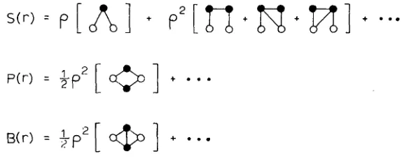
and B are the sums of the series, parallel, and bridge diagrams, respectively. The expansions of these functions, through Expansion of the integrand in (4) in products of Mayer

f ( r ) = e-flp(r)

-

1

g(r) e f l P ( 7 ) = 1

+

S ( r )

-+

P ( r )

+

B(r),

B(r) =

$p’[

c@]

+

...

Figure 1.

diagrams, through second order.

Density expansions o f the series, parallel, and bridge sets of

terms of second order in the density, are shown in Fig. 1 in the usual diagram notation.

In

addition, one defines a direct correlation function C ( r ) by the relation

( 8 )

= C(r)

+

S(r). (9)

G ( r ) E g(r)

-

1

Because diagrams of the series type can be factored in Fourier transform space, while those of the parallel type can be factored in

direct space, both the series S and

P

can be summed into simple functionals of g. These are(1)

~ ( r ) = p

J

c(r!)G(l

r - r!

1)

dr’

₍₁₀₎

(11) and

P(T) = g(r) eflC(7) - 1

-In

b(.)

eflq(*)].

(7)

P R E S S U R E - C O N S I S T E N T E Q U A T I O N 8 3

Equations (9)

and

(10) constitute the Ornstein-Zernike equation

G ( r ) = C ( r )

+

p

S

C(r’)G(

I

r

-

r‘

I)

dr’,

which yields G when

C

is known, while from (7) and (9) it follows that

C =

f(

1

+

8 +

P

+

B)

+ P

+ B ₍₁₃₎

= gePQf

+ P + B

(14)

= G - l n g e @ Q + B , (15)

where the last equality is a consequence of (11). It is apparently not possible to express B as a simple functional of g, so that a closed set of equations is not achieved and approximations for B must be introduced. Among other things, this leads to inconsistent values

of the equation of state as obtained from Eqs. (2) and (3).

The best known of these approximations are the PY and

HNC

equations, which are obtained by putting, respectively,

R ( r ) = - P ( r )

(PY)

(16)

B(r) = 0.

( H w

(17)

C = gef’qf (PY) (18)

C

= G -1ngePQ. (HNC) (19)

The corresponding direct correlation functions are then

The

fact that the PY equation, despite its neglect of an additional set of diagrams, leads to results that are generally superior to those of the HNC equation suggests that a partial cancellation occurs among the diagrams such that

P

+

B

is more nearly negligible than B alone.

We now consider a generalization of these cases that may more accurately represent the small correction

P

+

B

while still retaining the basic computational simplicity of the above equations. Define

the ratio

so that the direct correlation function is now written

C

= G + m ( g e P q - l ) - ( l + m ) l n g e a Q . (21)

(8)

84 F . L A D 0 A N D S E W - H S I A C E E N

I n this form, the PY and HNC equations result from the choice m(r) = - 1 and m ( r ) = 0, respectively. Other possibilities may now be explored, however. For example, a choice of m with no functional dependence on r but designed to yield a consistent value for the pressure from both Eqs. (2) and (3) leads to a significant improvement over the PY and HNC equations for hard ~ p h e r e s . ( ~ ~ J ~ ) This approximation, previously called pressure-consistent

(PC),

can in turn be easily extended t o include a spatial dependence for m ( r ) , as will now be shown.

Write the density expansions of

P

and B in the form

so that the exact m ( r ) is written

More genemlly, the expansion of m(r) may be written

where

or, in diagram notation,

and where

(9)

for

k

>

1 . Clearly, the expansion (251, though formally exact, is of no direct utility since the coefficients crk(r) are not readily obtainable. The approximation we propose consists in simply neglecting the r-dependence of these coefficients, thus letting mo(r) approximate the entire spatial dependence of m ( r ) , and determining the now- constant coefficients aB by requiring consistency in the equation of

state as calculated from (2) and (3). It is worthwhile noting that this approximation represents B(r) as a particular infinite series and is not a t all analogous to the straightforward extension of the HNC equation obtained by approximating B(r) by pzBz(r), rather than zero.

There remains the problem of determining the integrals in

mo(r).

For hard spheres, analytic evaluations of these diagrams are already available in the literature.(l6) In general, however, these integrals will need to be evaluated numerically, using Fourier transforms for P2(r) and Monte Carlo integration for B,(r), for example. It will, of course, be necessary to perform these calculations only once for each isotherm studied.

3. Virial Expansion for Hard Spheres

When the exact density expansions of g and C are used in (2) and (3), respectively, both equations yield the same virial expansion for the pressure of the fluid,

a consistency that is lost when approximations are introduced. The

PY

and HNC equations, for example, become internally inconsistent in this sense at the fourth virial coefficient D.

With the approximation

00

m ( r ) =?AT)

{

1

+

c

pk% ? (30)

E = l

}

the fourth virial coefficient is exact and the remaining coefficients can be made consistent, though approximate. The first few such coefficients can be readily calculated for the hard sphere model, where the diagrams needed for mo(r) have been analytically

(10)

86 F . L A D 0 A N D S H U - H S I A C H E N

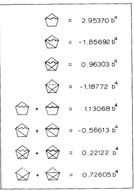
evaluated.(16) Many of the virial diagrams required for this caleu- lation are also available in the likratture.(l') Those not already available were computed, either analytimlly or numerically, and are listed in Table 1 with their numerical values.

TABLE 1 Additional Virial Diagrams Needed for the Calculation of the Fifth Virial Coefficient of Hard Spheres Using the Approximation of Eq. (30). Solid lines denotef(r), dashed lines rf'(r), and wavy lines m,,(r). The first four diagrams were evaluated analytically, the last four sets numerically. b is $wcrS.

6 =

2 . 9 5 3 7 0 b 4

@

=

- 1 . 8 5 6 9 2 b 4

@

=

0,96303 b4,

=

-1.18772 b"

6

+

=

1.13068b4

f

@

+

@

=

-0.56613 b4

@

+

@

=

0 . 2 2 1 2 2

b4

f

&

+

6

= 0 . 7 2 6 0 5 b 4

The hard sphere mo(r) is pictured in Fig. 2, from which one sees that mo(r) takes on the PY value of - 1 for r / u 2 J 3 , where u is the hard sphere diameter. (Actually, mo(r) for this potential becomes undefined for r / u

>

2, since both numerator and denominator of

(11)

0 1

.o

t-10 2

.o

Figure 2. The function m&) for hard spheres of diameter u.

(27) vanish. We have extrapolated the value - 1 which holds between r / o = J3 and r / a = 2 t o define mo(r) for values of r / o greater than 2.) Given this property of mo(r), it is clear that in the present approximation, the sum

(31) will be a relatively weak correction to the

PY

form of the direct correlation function, as expected. Note, however, that C will no longer vanish for values of r greater than a hard sphere diameter, as it does in the

PY

approximation.

With the numerical values of the required diagrams in hand, it is a straightforward, though increasingly tedious, task to determine the constant coefficients ak required for pressure consistency. We have

evaluated, under this condition, the first coefficient ul, which givea

P ( r )

+

B(r)

= [ 1 + m(r)]P(r)

m ( r ) = mo(r){l -0.1123bp+ . a * } (32)

for hard spheres, where b

=

37r03. This is sufficient to yield consistency through the fifth virial coefficient. The values of the fourth and fifth coefficients resulting from (32) are listed in Table 2, along

(12)

88 F. L A D 0 A N D S H U - H S I A C H E N

with the corresponding results of the PY,

HNC,

and

PC

equations given by Rowlinson.(16)

As

mentioned earlier, the fourth virial coefficient is now exact, while the fifth is clearly an improvement over the other three equations.

TABLE 2 Fourth and Fifth Virial Coefficients for Hard Spheres.

Exact 0.28695 0.1103

Eq. (30) 0.28695 0.1051

PC 0.2824 0.1041

PY V 0.2500 0.0859

C 0.2969 0.1211

HNC V 0.4453- 0.1447

C 0.2092 0.0493

For a dependable comparison at higher densities, a complete numerical solution of the integral equation must be obtained. These results are presented in the next Section.

4. Numerical Solufions for Hard Spheres

The nonlinear integral equation for g which results from Eqs. (12), (21), and (30) may be solved iteratively using Fourier transforms. The details of the numerical procedure for this calculrttion have been described previously.(lSJ*) As before, the equation was solved for g in the form

H ( r ) = r [ g ( r ) efl'(7)

-

11, ₍₃₃₎ evaluated at a finite number of discrete points r j . Iteration was continued until the largest difference between two successive iterates of H was less than

In addition, the pressures computed from

the virial Eq. (2) and from a Simpson's rule integration of the inverse compressibility ( 3 ) were required to have a relative difference smaller than 5 x 10-4. Calculations were performed in double precision on an IBM 360175.

With these criteria, solutions were obtained for the hard-sphere model at reduced densities pa3 = 0.1(0.1)0.8. The computed equation of state is listed in Table 3, along with the values obtained from the Ree-Hoover P ( 3 , 3 ) approximant(1Q) (which we take as a, reasonable

(13)

P R E S S U R E - C O N S I S T E N T E Q U A T I O N 89

TABLE 3 Hard Sphere Equation of State Computed from the Extended Pressure-Consistent Equation (EPC), the RegHoover P(3,3) Pad6 approxi- mant (RH), and the earlier Pressure-Consistent Equation (PC).

BPIP 0.1 0.2 0.3 0.4 0.5 0.6 0.7 0.8 0.976 0.953 0.903 0.860 0.826 0.781 0.726 0.680 1.240 1.553 1.967 2.516 3.252 4.252 5.624 7.539 1.240 1.554 1.968 2.521 3.268 4.291 5.714 7.732 1.240 1.553 1.966 2.513 3.246 4.239 5.605 7.513

" standard solution ") and the earlier pressure-consistent

(PC)

equation.(lS) It is clear from this table that the EPC equation gives

a, small but noticeable improvement over the earlier version. (These latter results in turn have been shown(13) to improve on the PY and

HNC equation of state.) The values of the density-dependent part of m(r) [see Eqs. (30) and (32)] needed to achieve a consistent equation of state are tabulated in the second column of Table 3.

R E F E R E N C E S

1. See, e.g., Rice, S. A. and Gray, P., The Statistical M e c h n h of Simple

Lip& (John Wiley and Sons, Inc., New York, 1965), Chap. 2.

2. Yvon, J., Actualit& Scientijique et Industriel, Vol. 203 (Hermann et Cie., Paris, 1935); Born, M. and Green, H. S., Proc. Royal SOC. (London)

A188, 10 (1946).

3. Rice, S. A. and Lekner, J., J. Che.,*. Phys. 42, 3559 (1965).

4. Mayer, J. E. and Montroll, E. W., J . Chem. Phys. 9, 626 (1941); see also Salpeter, E. E., Ann. Phys. (NY) 5, 183 (1958).

5. Van Leeuwen, J. M. J., Groeneveld, J. and DeBoer, J., Physica 25, 792 (1959); Meeron, E., J. Math. Phys. 1, 192 (1960); Morita, T., Progr. Theoret. Phys. (Kyoto) 23, 385 (1960); Green, M. S., J. Chem. Phys. 33, 1403 (1960); Rushbrooke, G. S., Physim 26, 259 (1960); Verlet, L., Nuovo Cintento 18, 77 (1960).

6. Percus, J. K. and Yevick, '2. J., Phys. Rev. 110, l(1958). 7. Stell, G., Phy& 29, 517 (1963).

8. Percus, J. K., Phys. Rev. Letters 8, 462 (1962). 9. Verlet, L. and Levesque, D., Physics 36, 254 (1967).

10. Metropolis, N., Rosenbluth, A. W., Rosenbluth, M. N., Teller, A. H. and Teller, E., J. Chem. Phys. 21, 1087 (1953); Wood, W. W. and Parker, F. R., ibid. 27, 720 (1957).

A 3

(14)

90 F. L A D 0 A N D S H U - H S I A CHEN

11. Alder, B. J. and Wainwright, T., J . Chem. Phys. 31,469 (1969); Rahman, 12. Carley, D. D. and Lado, F., Phys. Rev. 137, A42 (1965).

13. Lado, F., J. Chem. Phy8. 47, 4828 (1967). 14. Lado, F., J . Chem. Phy8. 49, 3092 (1968). 15. Rowlinson, J. S., MoZ. Phys. 9, 217 (1965).

16. Nijboer, B.R. A. andVanHov0, L., Phys. Rev. 85,777 (1952); Ree,F.H., Keeler, R. N. and McCarthy, S. L., J . Chem. Phy8. 44, 3407 (1966). 17. Rushbrooke, G. S. and Hutchinson, P., Physica 27, 647 (1961); Uhlen-

beck, G. E. and Ford, G . W. in Studie-s in Statistid Mechanh, Vol. 1 (North Holland Publkhing Co., Amsterdam, 1962); Rowlinson, J. S.,

Proc. Roy. SOC. (London) A279, 147 (1963).

18. A more detailed presentation of the quadrature rules used in the numerical Fourier transforms may be found in Lado, F., J . C q . Phys. (to be published).

A., P@8. Rev. 136, A405 (1964).

19. Ree, F. H. and Hoover, W. G., J . Chem. Phys. 40, 939 (1964).