Analysis and Analogue Computer Representation of commutating machines and its application to control systems.

Electronic Theses and Dissertations

Theses, Dissertations, and Major Papers

8-13-1965

Analysis and Analogue Computer Representation of commutating

Analysis and Analogue Computer Representation of commutating

machines and its application to control systems.

machines and its application to control systems.

Tilak Raj Sahni

Follow this and additional works at: https://scholar.uwindsor.ca/etd

Recommended Citation

Recommended Citation

Sahni, Tilak Raj, "Analysis and Analogue Computer Representation of commutating machines and its application to control systems." (1965). Electronic Theses and Dissertations. 6402.

https://scholar.uwindsor.ca/etd/6402

ANALYSIS AND ANALOGUE COMPUTER REPRESENTATION

OF COMMUTATING MACHINES AND ITS

APPLICATION TO CONTROL SYSTEMS

by

TILAK RAJ SAHNI

A Thesis

Submitted to the Faculty of Graduate Studies through the Department of Electrical Engineering in Partial Fulfillment

of the Requirements for the Degree of Master of Applied Science at the

University of Windsor

Windsor, Ontario

INFORMATION TO USERS

The quality of this reproduction is dependent upon the quality o f the copy

submitted. Broken or indistinct print, colored or poor quality illustrations and

photographs, print bleed-through, substandard margins, and im proper

alignm ent can adversely affect reproduction.

In the unlikely event that the author did not send a com plete m anuscript

and there are m issing pages, these will be noted. Also, if unauthorized

copyright m aterial had to be removed, a note will indicate the deletion.

®

UMI

UMI Microform EC52583

C opyright 2008 by ProQ uest LLC.

All rights reserved. This microform edition is protected against

unauthorized copying under Title 17, United States Code.

ProQuest LLC

789 E. Eisenhow er Parkway PO Box 1346

APPROVED BY:

a . l

The purpose of the present study is two-fold:

i) to present a unified approach for the analysis of both D.C.

and A.C. commutating machines,

li) to present the rigorous mathematical model and Analogue Computer

Representation of both D.C. and A.C. commutating machines.

I

The analysis begins for an ideal machine with the following

assumptions:

i) The air-gap flux density wave to be sinusoidal

ii) The effects of the coil short-circuited undergoing commutation

to be ignored.

iii) The magnetic path to be unsaturated

But in the actual machine, the following problems are encountered:

i) The air-gap flux density wave is non-sinusoidal

ii) A coil undergoing commutation is short-circuited

iii) The magnetic path is saturated

To overcome these problems, the voltage-current equations are

modified as stated below:

i) The presence of space harmonic components in the air-gap flux

density wave modifies the voltage coefficient in the

speed-voltage terms.

ii) The proper choice of the rotor and stator axes takes care of the

effect of short-circuited coil undergoing commutation.

iii) The saturation in the magnetic path causes the non-linearity in

coefficient by a factor S which is found from the open circuit

characteristic of the machine. This non-linearity can be

simulated in the Analogue Computer Representation by a function

generator.

Finally, an application of D.C. commutating machines is shown in

the position control system.

The sincerest appreciation of the author is extended to Dr. H.H. Hwang

for his generous provision of guidance and encouragement, and for the

wealth of knowledge which he made available to this work. Thanks are

due to Dr. P.A.V. Thomas for the encouragement from time to time during

the work.

Special thanks are directed to the National Research Council which

TABLE OF CONTENTS

Page

ABSTRACT... iii

ACKNOWLEDGEMENTS... v

TABLE OF C O N T E N T S ... vi

Chapter I. INTRODUCTION... 1

II. Generalized Theory... 2

III. D.C. COMMUTATING MACHINE... 13

IV. A.C. COMMUTATING MACHINE... . . . . . 36

V. CONCLUSION... 45

REFERENCES... 46

The characteristics of variable speed with change of armature

voltage of a D.C. machine have led to its many important uses. Its

superiority is shown over other types of machines in the control system

application. In the position and velocity control, D.C. machines are

used in mose cases.

Therefore, such a need of a D.C. machine has led to its rigorous

study and its representation by a mathematical model. The analysis is

proceeded with two axes (d-q axes) theory and, therefore, a most general

D.C. machine, having field and armature windings and brushes placed on

both the axes is studied.

In the study of commutating machine, the following three difficulties

are encountered:

1. The Air-gap flux density wave is non-sinusoidal.

Z. A coil undergoing commutation is short circuited,

3. The Magnetic path is saturated.

In the present study, all these factors are taken into special

consideration. The Analogue Computer representation has been presented

for a general machine known as a Metadyne and then for an Amplidyne. An

application of the D.C. Commutating machine is shown in the position

control system.

Further analysis has been proceeded to study the A.C. Commutating

machines, such as the Repulsion Motor and the Single phase A.C. Series

CHAPTER I I

GENERALIZED THEORY

2.1 Ideal Machine

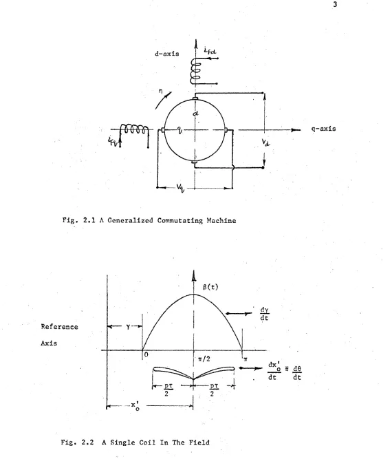
A most general commutating machine, shown in Fig.2.1, represents

windings as equivalent coils placed on two orthogonal axes. All the

windings shown either exist physically or represent an equivalent of

some phenomena occuring in the machine. It is possible that there may be

more or less number of windings that those shown on each axis. There are

also two sets of brushes placed 90 electrical degrees apart on the commuta­

tor for generalization, which are actually present in the cross-field

machines.

The two orthogonal axes shown in Fig.2.1, are chosen as stationary

axes and defined as

i) Direct Axis (or Pole axis) - Axis of the main field winding.

ii) Quadrature Axis (or Interpolar axis) - An axis 90 electrical degrees

ahead of Direct-axis. Sometimes it is known as the Brush Axis.

The analysis begins with an idealized machine and later is modified

when actual difficulties are encountered. Hence it proceeds with the

following assumptions:

i) The Air-gap flux density wave to be sinusoidal

ii) The Magnetic path to be unsaturated

iii) Hysteresis and Eddy current losses to be neglected

iv) Effects of the coil to be short-circuited as commutation is to be

ignored.

With the above stated assumptions, the voltage induced in the coil

Fig. 2.

Reference

Axis

Fig. 2.

d-axis Lfd,

>»_ q-axis

L A Generalized Commutating Machine

rr/2

£ 1 £ 1

de

4

whose centre is located at x^ from the reference axis is to be found.

Here the most general case is considered so that

i) flux density is a function of time

ii) flux density is moving with the velocity of d^ dt

iii) A coil of short pitch pT is placed on the armature which rotates with

a velociey d 6 . dt

To find the voltage induced in the coil, the flux-linkage with the

coil is first found and then its time-derivative is taken to find the

induced e.m.f.

Therefore, flux embraced with the coil,

1 v ti

2 X

3 dx dy

JL

2 x . .2.1

1 - axial length of armature

x ? and x" - distances of two ends of the coil from the

reference axis

6 - flux density which is a function of time and space; and

it is given as

3 ■ 3 sin

m firx + y

2t . K K 3 sin d> = — 1 p s m T ir

t tx' + y

where K " sin ^ - pitch factor

p 2

2t 1 . firl .

K ■ — --- sin j— tan s irl tan a

..

..2.3

..2.4

tan aj- skew factor ..2.5

or 6 « K K 1 sin P 8 ®

2t

where $ “ — I B ....

Tm ir m

..

..2.7

from the equation 2.6, it is seen that flux embraced by the coil is a

function of <b , x", v i.e., Tm ’ o ’

f * f

. .

The voltage induced in the coil,

c

..2.9

-N K K p s

U L a dt

firx' \ sin}— j a + Y ).

m

dx1

1T_ _0 + i x cos __ o + TTX* y

x 5t • dt

J

..

Consider a group of q coils uniformly distributed in slots separated by

a slot angle a and the centre of the group is located at xq from the

reference axis. The voltage induced in the group of coils is,

e - -N K K K q f ^ m sin p s d

dt

TTX o + y

+

7f dx

— o

«

+ «±- cos

f *

TTX ,

o + y } •*2*11

T dt dt _y

, T

and - winding factor

Effective number of turns

. .

6

ip * N <p - flux linkage

m e m ..2.14

The equation 2.11 can be rewritten as

e * - ( ^ m sin

fit

fix

TTX

o + y

m T 51 fit

0 ,

cos

/

— + Y

> 4

..2.15

The three terms in equation 2.15 are interpreted as

i) The term 6^ represents transformer e.m.f.

fit"

ii) The term fixQ represents speed e.m.f. due to movement of conductors.

fitT

iii) The term fix represents speed e.m.f. due to movement of field.

f i t . .

In all the commutating machines, the field must be stationary while

the armature is rotating.

Thus dx “ 0 ..2.16

dt

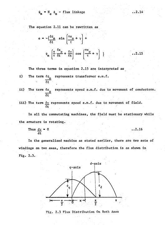
In the generalized machine as stated earlier, there are two sets of

windings on two axes, therefore the flux distribution is as shown in

Fig. 2.3.

q-axis

or

Thus the flux at any point is

<|>(x) “ <j)^ sin + <}><j s i n ,.2.17

4

The voltages e^, e^ induced in the windings placed on d-axis and

q-axis are respectively

1 ^ 4 . , - 4 a

ed " dt *q dt ..2.19

dfl d»c

e, * - * d d ? - d T ..2.20

The armature terminal voltages are

^ d d A

v ■ e - i r * - -j— + ii — - i r . .2.21

d d d a dt dt d a .

r)A

v - - e - i r ■ - ♦ . f - / - i r ..2.22

q q q a a dt dt q a

The flux linkages ^ and can be written in terms of self and

mutual inductances of the coils on the two axes, for in the unsaturated

magnetic path, a linear relation between flux linkage and the current

exists.

2.2 Practical Machine and Problems Encountered

In the previous section, theory is developed for an ideal machine

under the assumptions made, but the machine is not ideal and a number of

problems are encountered in the actual machine. It is difficult to

develop the theory for an actual machine, therefore, a theory is first

developed for an ideal machine where the equations are obtained in

correct form and then certain factors are modified for the actual

machine. The following problems are encountered in the actual commutating

machine:

8

2. The coil undergoing commutation is short-circuited

3. Saturation of the magnetic path

1) Space-harmonics in the air-gap flux

density:-The flux density distribution in the air-gap is not sinusoidal but

it contains space harmonics. The equations for e.m.f. induced are

derived on the assumption of a fundamental air-gap flux density. By

inspecting the voltage equations (nos. 2.21 and 2.22), it is found that

they contain two terms - (a) Transformer-voltage - and (b) speed-voltage

, a e

d t

The speed-voltage term is more predominant than the

transformer-voltage term. Thus the correction for transformer-transformer-voltage is not of

much importance. To modify this term a lot of problems are involved in

finding the exact flux density wave shnpe, its harmonic component and

the voltage due to each component. This process is very labourious and

the result can be obtained with sufficient accuracy by considering only

the fundamental component.

d 0

The second term is speed-voltage, — where flux linkage \f/ is of

the form ip = Mi ..2.23

where M is mutual inductance in the case when only fundamental component

is considered. For for non-sinusoidal flux density M does not remain as

the mutual inductance coefficient but is to be modified. This coefficient

is known as speed-voltage-coefficient-G which is to be found experimentally.

Thus the voltage equations (2.21) and (2.22) become

• •2.24

2.25

where X , and X are of the form X

2) Short-circuited Coil Under Commutation.

During the process of commutation, coils are being short-circuited.

These short-circuited coils set up a field in the air-gap. The coils

short-circuited by brushes placed in the d-axis produce a field in the

q-axis, and vice-versa. Thus the effects of short-circuited coils can

be considered along with the fields in both the axes while measuring the

constants of the machines. This line of approach is true only when the

axes of the rotor are chosen to coincide with the corresponding axes of

the stator.

3) Saturation of Magnetic Path.

In the actual -machine, the magnetic path is considered saturated

&nd in fact in the self-excited D.C. machine the magnetic circuit must be

saturated). The saturation has two effects: (1) reduction of inductance

and (2) reduction of voltage generated in the armature circuit.

The effect of saturation can be considered with the approximation

that there is no interaction between the flux at the d-axis and that at

the q-axis. Recalling the relation

^mdf * ^ ^Vqa^oc ..2.26

n

where ^ “ field flux linking with d-axis circuit

A - Constant of proportionality

(Vqa)oc “ Open-circuit armature voltage in q-axis

n - speed in radians per sec.

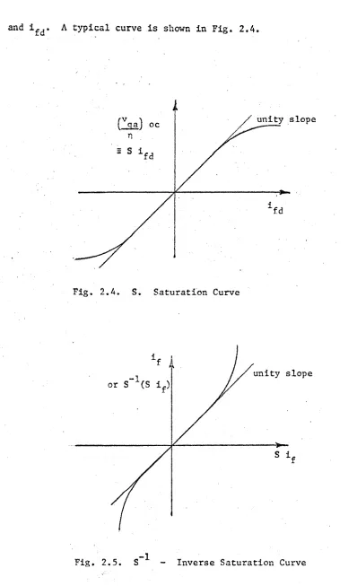
A curve between the d-axis field current, and the q-axis open-circuit

armature voltage per radian per second of speed will give the measure

and ifd« A typical curve is shown in Fig. 2.4.

unity slope fVqa) oc

Fig. 2.4. S. Saturation Curve

unity slope

The self inductance of the field winding is related as

Lfd " Lfld + Lmfd

where 1 ^ ^ is inductance due to leakage flux which does not link with the

armature circuit and L is the inductance due to mutual flux and it is m f d .

Lm f d " ^ ..2.28

h i

Hence, a relation between open circuit voltage and inductance is

established as given below.

A jlga] ~ T -• - L

— " A i d f H Lmfd xfd = ifd ..2.29

n mfd

a S i

& I fd

" I s L if j

g7: fd

af

where is inductance of unsaturated portion and is considered to be

constant.

Because of saturation, the flux is reduced and hence the speed

voltage is also reduced. This is allowed for by the speed-voltage

coefficient G ^ , and which is a constant speed-voltage coefficient

found from the unsaturated conditions. Therefore, by finding S which is

a function of field current, the values of

Lmfd * S Lmfd

and G . * S G',

af af

can be obtained.

Thus in the voltage equations, mutual inductance coefficients and

1 2

CIS

for finding the differentials, the term “ is assumed to be negligible.

Hence the effect of saturation is appropriately accounted for. In

Analogue representation, the inverse saturation factor S ^ is required

which is defined by interchanging the axes of Fig. 2.A. Thus S ^ is

obtained in the Fig. 2.5. In the analogue representation, this can be

represented by a function generator.

In the two axes machines, two saturation factors S, and S

d q

(or S, * and S are defined for two axes. The S,1 is determined from

a q a

(v ) versus the direct axis field current i,,, and S ^ is determined

qa oc fd q

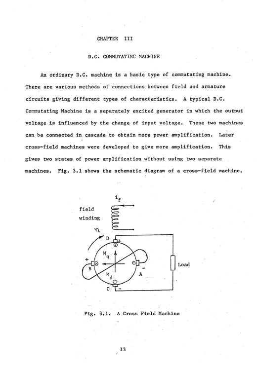
An ordinary D.C. machine is a basic type of commutating machine

There are various methods of connections between field and armature

circuits giving different types of characteristics. A typical D.C.

Commutating Machine is a separately excited generator in which the output

voltage is influenced by the change of input voltage. These two machines

can be connected in cascade to obtain more power amplification. Later

cross-field machines were developed to give more amplification. This

gives two states of power amplification without using two separate

machines. Fig. 3.1 shows the schematic diagram of a cross-field machine.

i f

field

winding

Load

1 4

With the armature running in clockwise direction, voltage of marked

polarity is induced in the brushes A and B. If these brushes are short

circuited, a large amount of current flows in the armature conductors,

setting up a M.M.F. - M in/the'direction shown, which produces flux

perpendicular to the main flux. If a pair of brushes C and D are placed

perpendicular to the axis of AB, voltage is induced in these brushes

C and D due to rotation of armature. The load can be connected across

the brushes C and D. This in short is a principle of cross-field machine.

These can be classified as two-stage machines also.

In general, a Metadyne generator can represent a cross-field machine.

Another type of cross-field generator is the Amplidyne in which compensating

windings are provided on the stator. These compensating windings carry

the load current and produce an M.M.F. equal and opposite to M^ (due to

armature reaction). Thus, the net flux remains constant. Therefore, the

Amplidyne is known as a constant-voltage generator. In the Metadyne, lack

of compensating winding results in negative feedback. The negative

feedback introduces two serious problems. There is much less power

amplification in Metadyne compared to Amplidyne. The problem of

oscillation is overcome by providing additional damping winding.

Another difference is that speed of response of Metadyne Generator

is rapid in comparison to the response of either a separately excited

D.C. machine or an Amplidyne. Eddy currents in the iron path, though

minimized by lamination, can . r ;., . :> -,ort circuited winding. Eddy currents have a small effect in transient response. Eddy currents,

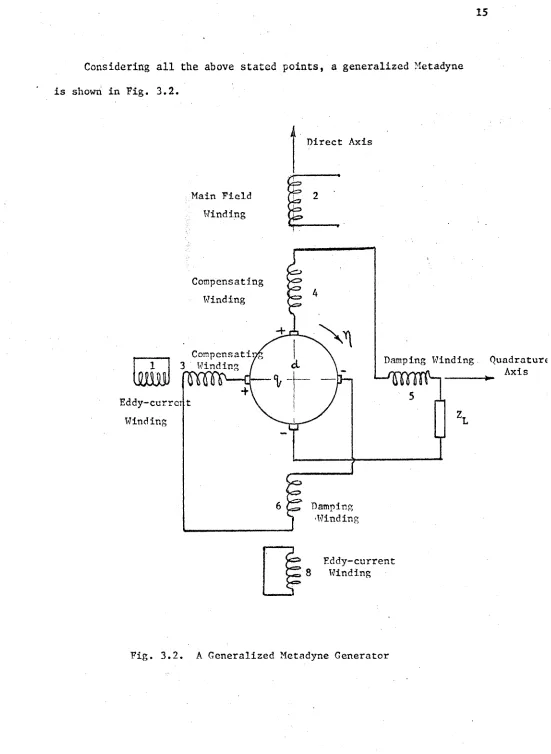
Considering all the above stated points, a generalized Metadyne

is shown in Fig. 3.2.

Direct Axis

Main Field

Winding

Compensating

Winding

Compensating

3 Winding ( Damping Winding

l o t

Eddy-currcr

Winding

Damping ■Winding

Eddy-current 8 Winding

Fig. 3.2. A Generalized Metadyne Generator

1 6

Direct Axis Windings:

2 - Main Field Winding

4 - Compensating Winding in series with the d-axis armature winding.

It produces an M.M.F. in the same direction as the M.M.F. of the

d-axis armature winding,

d - Direct axis armature winding

$ - Damping winding connected in series with the q-axis armature winding

and placed in the d-axis

8 - Short-circuited fictitious winding f o r eddy current path in the

d-axis

- Load Circuit

Quadrature Axis Windings:

1 - Short circuited fictitious winding for eddy current path in the q-axis

3 - Compensating Winding in series with .the q-axis armature winding. The

M.M.F. is in the direction of the M.M.F. due to the q-axis armature

winding.

q - Quadrature-axis armature winding

5 - Damper winding in series with the d-axis winding and placed in the

q-axis

As found out in the previous chapter, the voltage induced in the

d-axis and q-axis windings are of the form 2.24 and 2.25, under the

condition of non-sinusoidal flux density distribution. But still, two

these e q u a t i o n si

1) Speed of Metadyne is constant

2) Magnetic circuits are unsaturated

Rewriting the equations 2.24 and 2.25

v, « - ^ d + X d0 - i,r , .

v 0 _ x i i . ^ ! a _ i r

v A , . « i r o o

q d dt dt q a ..3.2

Thus, to derive the voltage equations, first the flux-linkage with

each circuit is found. The subscript denotes the corresponding circuit;

*2 " L 2i2 + M 42x4 + M d2id + M 62i6 + M 821 8 ” 3,3

*4 " M 2Ai2 + V 4 + '^d4id + *64*6 + M 84i8 ‘ ‘3 ‘4

^d " ^ d ^ + ^ ^ 4 + + M 6di6 + M 8di8 •*3 ‘5

^6 " M 62i2 + M 64i4 + M 6did + L 616 + M 68i8 **3,6

^8 “ M 82i2 + + M 8did + M 86i6 + L 818

t|>, - L.i, + M , 0i0 + M, i + M.-i. ..3.8

1 1 1 13 3 lq q 15 5

- M,.i. + L,i_ + i + M,-i. ..3.9

3 31 1 3 3 3q q 35 5

ip = M _i. + M _i_ + L i + M i ..3.10

q ql 1 q3 3 q q q5 5

■ M-.i. + M c0i0 + M c i + L ci c ..3.11

5 51 1 53 3 5q q 5 5

Coefficients for speed terms:

X, = G i + G i + G i + G i + G i ..3.12

d 2 2 4 4 d d 6 6 8 8

X - G i + G i + G i + G i ..3.13

S 1 1 3 3 q q 5 5

Now voltage equation for each of the circuits is shown in the

V 2 “ V 2 + P L 212 + pM42^4 + pMd2*d + pM6216 + pM82i8

..3.14

v 4 ““pM 24i2 “ pL4i4 “ pMd41d” pM64i6 " M 84i8 “ r4*4

..3.15

vd “ ”pM2di2 “ pM4di4 “ pLd Ad ** pM6di6 " pM8d18

+ ( + 03i3 + Oqiq + G5i5) n - idrd •-3 -16

v 6 “ “ pM62i2 “ pM64i4 " pM6did “ pL6A6 "pM 86i8“ i6r6

•..3,17

v 8 * “pM82i2 ” pM8414 “ pM 8did “ pM8616 -‘pL8i8* i8r8

..3.18

V 1 “ *pLlil ~ pM1313 “ ^ V q “ pM15£5 “ V l ,,3,19

v3

• * 3 * 20

v q - -<G2i2 + Ga14 + Gdid + G 61 6 + Gglg) D

" ^ q l 1* “ ^ 3 * 3 “ pLq *q ~ “ V a ..3.21

v 5 - - •pM51i1 - pM53l3- pM5qiq - pL5l5 - i5r5 ..3.22

..3.23

L

For open-circuits^and steady state case, speed voltages are:

v ■ - (G0i0 + G.i. + G.i, + G,i, + G Qi_) n ..3.25

qo v 2 2 4 4 d d 6 6 8

when saturation is considered, the equations 3.24 and 3.25 are modified

to:

v do - (+ ‘H 1! + «313 + " S, ••3 ‘26 '

v - - + * % + ° ; ° 6 + ^ s ) 11 sd ••3 -27

3.2 Analogue Representation of Metadyne

The Metadyne with all these windings can be simulated on an Analogue

Computer. For the Analogue representation, the equations 3.14 through

3,23 are modified under the following conditions:

1) The self-inductance of each winding can be written as a sum of

leakage inductance and mutual inductance. Hence for Kth winding

^ " LK1 + LKK ..3.28

where is leakage inductance of winding due to leakage flux, and it

is assumed to be constant, and L v is mutual inductance of winding K due KK

to mutual flux. The mutual inductance is defined as * ^m

h

..3.29

where - mutual flux and i^ - current in the winding.

2) Same mutual flux links with all the windings on the same axis. This

assumption is reasonable because all the field windings are physically

wound on the same structure. This condition results in the following

relations:

- p - LK1 o

t

2 0

where N„ and N are the number of turns in windings K and j respectively.

K j

3) Since the speed voltage is proportional to mutual flux, and mutual

flux being the same for all the windings, a relation among speed

coefficients is;

o f i NK n .

..3.31

4) Speed of amplidyne is constant

5) The equations and Analogue representation diagram are first derived

on the assumption of no saturation and then are modified later for satura­

tion according to Chapter II.

By substituting equations 3.24, 3.25, 3.28, 3.31 into equations

3.14 to 3.23, the following relations are obtained

©x

VA

- p

L // v, “ p 44 4 K p—

4 v _a° h

(i

\ G i - - °414 + p ^44 _{_}V_2° n .

,3.33

or

v, « ^^dd

d

^7

_3° + v _do - Z i_{d d}

V d “ Vdo G, - - G.i, + pLdd

_ _ _ d d d

v qo n

or

₁₆

6

6

p L 66 - G

616

V go.

n ..3.35

v

8

“ G 8 i 8 +

pL

88 _{-3° ..3.36}

Adding equations 3.32 through 3.36,

- V

2

6

Z2 Z4 Zd d

Z6

6

Z8

8

”G2i2” G4i4 ” Gdi8 ~ G6±6 ~ G8i8 + pL22 + pL44

Z2

+ pLdd + pL55 +

pI88

Z 4 _d z_d , z *

6

v

v

+ P

L22

pL66

p~88

Z2

iL ~Z, V qo n ..3.37 Quadrature-Axis pL v = - l.Z.

1

11

11 do

n

or v pL.. ! v

~ ' Gi = - V i " T T

zi 1

do

n

..3.38

v 3 i3Z3 "

2 2

or

or

or

12

3

3

3

v * v - P^qq K do

q

q°

LA

- i Z q q

pL 33.

v do

V 5 =

v

5g5

55

- irG do

pL 55 ■5 5 . Z t

do

.3.39

.3.40

.3.41

Adding equations 3.38 through 3.41,

v. v,G_ v - v

3 3 , q qo V s

c„ + H r

2

li.G. + i.G, + i G + i-GJl 1 1 1 3 3 q q 5 5J

+

PL11

7

_

1

₅

„„

*

--V do + pLll + pL33 + pLqq + r h i '

li, v i_do

n Z1 Z3 Z_q Z5 _ _{q .}

**• ..3.42

Referring to Fig. 3.2, the following relations also exist.

..3.43

-v x -

0

0

*3 " *6 * \

v- + v + v- =

0

3 q

6

..3.44

..3.45

or

v. + v, + v_ + v_ “

0

4 d 5 L

v4 + v5 + Td ..3.47

Thus the equations 3.37 and 3.42 are modified to:

v oG o j.v /g / j. " v j o j. v c.G a - 2 2 + 4 4 + d do G, +

6

6

T-

P^oo . Pk/,/, , P^jj P

l-sf-7. z.

2 4

V

m +

h

pL88~

V

n

J.48

V _ G _ v - V

3 3 + q . £ £ q + 5 G rG j. v c r

Z5

= _

V do pLll + pL33 + pLao + pL55~ V do

n z z z z

3 3 9

5

n ..3.49

Effect of

Saturation:-As discussed in Chapter II, the effect of saturation is considered

in the analysis of the machine. In this case saturation is effective on

both axes and so the coefficients of saturation (S) are found out

separately for the d-axis (S^) and the q-axis (S^). is found by

measuring the rotor open circuit voltage on the q-axis when a current is

passed in the stator-circuits of the d-axis, and similarly is found by

the d-axis open circuit voltage with a current in the q-axis stator circuits,

Thus the equations 3.32 through 3.49 are rewritten, taking the

saturation into account.

or

v2 - z2i2 - I k

p

*2

V

L n .

_a°

. .3.50a

2 4

T '

v 4~ ' Z 4i4 + - i i P G 4

v go

n ,3.51a

or

V ' i G.'i. + L«i

4 — p

4 4

V

22

v j_d ~ _{do d d} + ^dd P_{—x t} G d

v

_22

n ..3.52a

or _{v j " v j}

d d

v

_22

..3.52b

L ' v, '■ - Z-l- +

66

6 6 6 “t t t P 6

v - 3 2

n ..3.53a

or

V 6G6

Z6 16i6 +

L 6 6

Z6 P

_ n j

0

T • +

88

G8

V

qo

_ h - ..3.54a

or

.

0

8i8

8

G8

fv ^

_22

. n _ ..3.54b

Adding equations 3.50b through 3.54b:

- V£ + Vi + v vdo G- + Vi

Z2

5*2

+ Gi

*4

+ CPd

+

GiV

+ %]

T t T » T * Y » T *

Z 2 1 + l i l dd +

l66

88

Z2 Z4 Zd

Z6

Z8

( \

V

P qo

I

-1

_3L2 _{+ ~ ~~ +}

[L22

L66

88

2 4 6 8 Z d

V p _ 3 2

Quadrature axis:

0 = - Z.i, - L11

1 1

-prr

or 0 ** - G'i,'- L 11

1

1

I .

v, * - Z_i„ - ^33

3 3 3

-pr

3

v do L n J

do

..3.56b

.,3.57a

or

do

v n ' ■ ■ T 1

3 3 » - Gli, - “33

— 3 3 — p

3

f < V

v - v = ! - Z - i - qq

q qo .

q q

q

.3.57b

..3.58a

or

Vq Vqo G ’ = - G'i - *Jqq

z q q q

q q

do

V , = ~.Z

1

5 5 5 pT p

5

do

..3.59a

or

V 5G5 , . , L55 5 5 ' ^ p

do

..3.59b

Adding equations 3.56b through 3.59b,

V 3C 3 + vq ~ t' + V 5C 5 '

z ,

z

q

z

3 q 5

- - (Gii, + Gli, + G'i + G'i ] ' ■ 1 1 3 3 q q _{q q} 5 5 V

L' L' L' L ’ ~

JL3L + - 1 1 + + z, z , z z ,

1 3 q 5

R

- - S

-1

z, z ,

z

- 1 3 q

5-do

..3.60

26

F W H — --A'

jo I in

►4 It

81

J

■

^i

q.

3

.1

A

n

a

l

n

q

u

e

Poo

re

sc

n

ta

t

i

o

n

of

‘to

t

a

/V

Thus with the help of equations 3.50 through 3.60, Fig. 3.3 shows

the Analogue representation for the Metadyne. The effect of saturation

on both the axes is considered in this representation. It contains two

integrators only, and the non-linear portions in the feedback paths can

be implemented with function generators*

Amplidyne

As stated earlier, the Amplidyne is a special type of Metadyne in

which compensating windings provide complete compensation in both the

axes. This results in a circuit without feedback. Thus in the absence

of feedback, the machine will be stable, contrary to the Metadyne, which

may be unstable. Therefore, damping windings are not required for the

2

Amplidyne. From the experiments conducted by Fegley , it is observed

that the effect of the eddy current circuit is negligible and thus the

fictitious short-circuit winding representing eddy currents can be

neglected. Therefore, the Amplidyne windings 5,

6

8

and the following relations apply:

Direct Axis:

V 2 " Z 2 ± 2 + pL22i2 " (R2 + 3.61

v 4 " “ pM24i2 " pL4414 " pKd ^ d ~ Z4i4 3.62

Vd " " p M

2

i2

• •3.63

v, + v, + vT *

0

or

or

₀

“ “ pM24i2 " pM2d12 “ pL44i4 “ ^ d ^ “ ^ 4 ^ “ pLdd1d

- V 4 - 5 S - [G 3 +

Gq)V

2 8

or

(

, + G ) n i

2. + Z, + Z_

4 d L

..3.64

Quadrature axis:

v

3

3

3

3

3

V q ” " (G

2*2

q q

..3.66

0

3

- pL_i« - pM i - R„i_ - pM ,i_ - pL i - i R G i. n

r 3 3 3q q 3 3 r q3 3 q q q q

2

0 » - (R_ + R +

1

3

<1

2

2

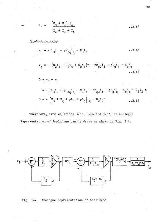
Therefore, from equations 3.61, 3.64 and 3.67, an Analogue

Representation of Amplidyne can be drawn as shown in Fig. 3.4.

V

2

Normally the magnetic circuit is not saturated, so the effect of

saturation is not shown in the Analogue representation, but if required,

it can be shown as discussed in Chapter II.

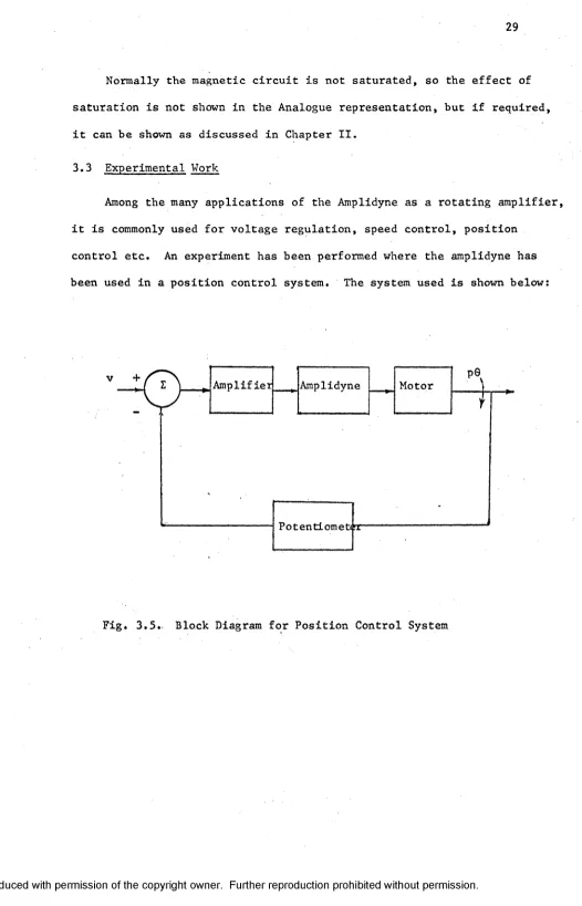
3.3 Experimental Work

Among the many applications of the Amplidyne as a rotating amplifier,

it is commonly used for voltage regulation, speed control, position

control etc. An experiment has been performed where the amplidyne has

been used in a position control system. The system used is shown below:

Amplifier Amplidyne __ Motor

p

6

PotentLomehir

3 0

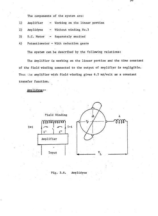
The components of the system are:

1) Amplifier - Working on the linear portion

2) Amplidyne - Without winding No.3

3) D.C. Motor - Separately excited

4) Potentiometer - With reduction gears

The system can be described by the following relations:

The Amplifier is working on the linear portion and the time constant

of the field winding connected to the output of amplifier is negligible.

Thus the amplifier with field winding gives 6.2 mA/volt as a constant

transfer function.

Amplidyne:-Field Winding

i n n n n f | T m r

I+i

Amplifier

Input

I - Direct current in the field winding when amplifier is balanced,

i - Signal current (alternating current in this case, because

‘input to the system is sinusoidal).

In this type of field connection, the flux-linkage with d-axis wind­

ing is found.

to. - - L.i, + M.-i' -'M.-i" + M.i.

rd d d df df 4 4

i* * I + i i" » I - i

*d - - V d + M df2i + M 4*4 ..3.68

Thus the equivalent field current is 2i. i.e. ±2 = 2i.

i, - 2 K.(v - K 0) . , ,Q

2 A p ..3.69

v, ® - p G i ..3.70

d q q

0 = - fR + pL } i - n G

0

1 9 9J 9

2

2

In the direct axis curcuit, the resistance and inductance are

taken in series with the armature of D.C. motor.

v j “ [Rj + R/ + R + Ph. + pL, + ph )i, + v

_0

1

1

- (R + pL) id + vb

« ^ P G ..3.73

» J P20 + ape ..3 .74

v = Sin u)t input signal to the system ..3.75

Taking the Laplace Transformation for both sides and sloving the

where . K ■- ( n G j .S,«2) 21^

a ■» JLL

q

b * aLL + RJL + JLR

q

q

q

3.77

c « RR J + aLR + RaL + K? L

q

q

d « R R o + K ? R

q

q

The output of the system, i.e. the angular position 0, is found in

the time domain by taking the inverse Laplace transformation of the

equation 3.76.

The constants of the system components were found experimentally and

are listed below:

Amplifier: = 6.2 mA/volt

Amplidyne: R , = R * 25.A ohms L, = L ■ 0.765 H

Nw. metre, sec/rad.

Potentiometer: K = 0.0198 volts per radian P

Input Voltage: 0.27 v at f ■ 0.1 c/s peak

These constants are substituted in the equations 3.76 and 3.77 and

Motor R^ * 24.2 ohms, = 0.58 volt sec./rad.

m

-4 2 -4

n >t ' r \ \ i i r>

t v - i I V »/ ^ . S '

,/ ,vnv \<

.;r ''. / . r ': :f'^ •" vs.*:

/ 7 A S

|r '

1

p - <4 T V. u i { 7 x

Sr -a ,* u n

t / / \ \

/' J _$

' ■* -£ £'T u V . a \ v -;;

r 7 r’ n " ' / ■ v* u ;-' \ '*v -j;

l L h V*« // 7 V '.

*■ / A \ t \v // . t ■■■. 5 >< A I \ \ Vi /r < ’ V:>,

Y J f , / iV V . / / " *\

s*«r • -r v v

B E ’ ' v '' '

BC t U

gu- ' \

BSSV J \ ‘'

1

in"-' v "i !

I? \

jr. • v \ '

ir * \ < \

, yf .

liv^* ,? ^ , *v'^-' ,>

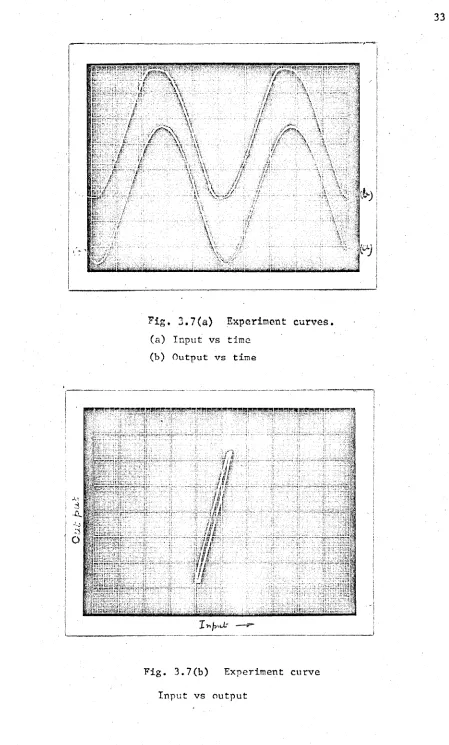
Fig, 3.7(a) Experiment curves,

(a) Input vs time

(b) Output vs time

j & )

<Pj

A‘

' n r r ^ ' n

-;T ir l i i s l

.

Inr* '-'r'j

1

I L : , , ; .

* -^Frr

ln .. (

l-r--:;-Jt li mx

jca.

t i p

u r . i f ;/h

>j'x ’

i t i

m " f/IC ’

r nr

/if i idl

' i t

u r '1/

i< /if

1 7 r-r

r

i«p

77:i|

, Jl

'11*4

j. 4

X »

Fig. 3.7(b) Experiment curve

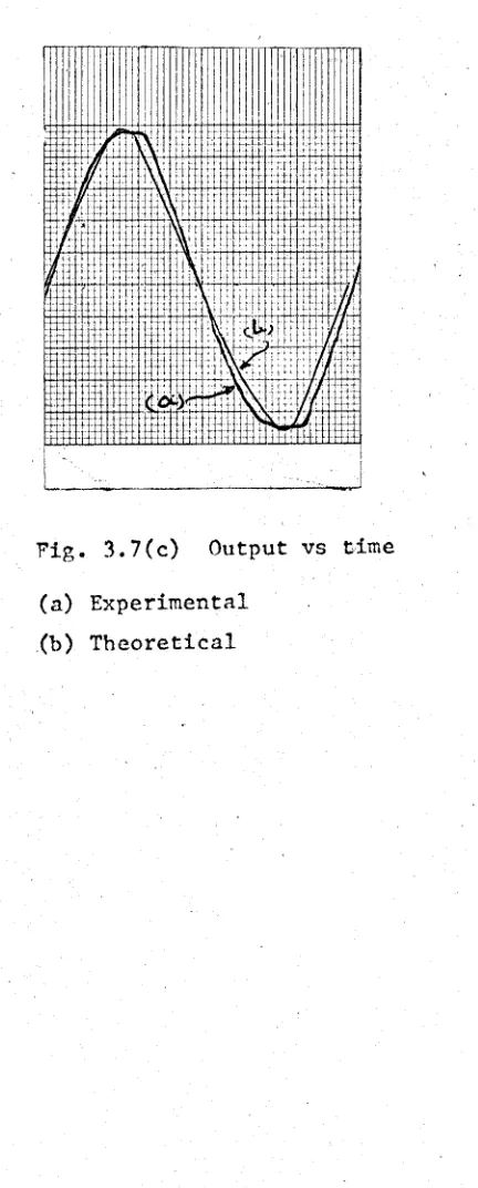
Fig. 3.7(c) Output vs time

(a) Experimental

0

0

time and compared with the experimental results in Fig. 3.7. From the

experimental results, it Is observed that the output curve is flat topped, while in the theoretical results, it is sinusoidal, but the

difference between the results is only 5 - 6 % maximum.

A curve between input and output is traced experimentally on the

CRO, and it appears like a hysteresis loop. It is found that the area

CHAPTER IV

A.C. COMMUTATING MACHINES

Though D.C. commutating machines were developed earlier and have

been commonly used, later A.C. commutating machines were developed and

used especially in traction and domestic appliances. A.C. commutating

motors have two advantages over the other A.C. motors: (i) its high

starting torque and (ii) its variable speed. These can be single-phase

and three-phase motors. Three-phase motors are used in traction while

single-phase motors are most commonly used in the domestic appliances.

The A.C. series motor is commonly known as a ‘Universal Motor*.

Series Motor

If instead of a D.C. supply, an A.C. supply is applied across the

terminals of a D.C. series motor, the motor will run, because the direction

of both flux and armature current changes simultaneously. But it is

observed that with the A.C. supply, the performance is poor - less

torque and poor power factor. The performance can be improved by reducing

the inductance of the windings. The field inductance can be reduced by

decreasing the number of turns on the field winding which results in less

flux and thus less torque. To get the same torque, the number of armature

turns is required to be increased. In this way, the armature inductance

is increased. A compensating winding can be provided on the q-axis which

produces an ra.m.f. opposite to that of the armature, and thus reduces

the effective inductance. Therefore, the performance will improve, i.e.

better speed regulation, more torque and better power factor.

Field Winding

q-axis

Compensating Winding

38

The A.C. series motor is shown in Fig. 4.1. The voltage equations

are given below:

v 2 ’ ‘ " V i ' V 2 ..4.1

5 J ’ ' ' V i ' V l ..4.2

Vq * •pMq313 " PV q * V ? + ^ 2 "

"''•3

T - Jpn + an - Iqr,2i2

i„ “ i _ = i .= i ..4.5

2 3 q

- V «* V « + V , + V

,

,

2 3 q , . .4.6

Substituting the equations 41., 4.2, 4.3 and 4.5 in equation

4.6, it is obtained,

v * p|l

2

3

2

3

..4.7/

With the help of these equations, an Analogue representation can be OWL

drawn,in Fig. 4.2 for an A.C. Series motor. A

Equivalent circuit:

Referring to equation 4.7, which gives the performance equation of

series motor, ai\ equivalent circuit can be drawn as shown in Fi^. 4.3.

Steady State Analysis:

Let the voltage applied to the motor as v = Sin wt,

and the current be i = I Sin (wt +cj>) m

forsteady state, the equations 4.4 and 4.7 are modified as

V - (r2 + r3 + *,)

1

1

4 0

2 2

The Electrical Torque developed T^ = G^I Sin (wt +<(>)

..4.9

1 2

and the average torque T = — G I

av

2

2

Repulsion Motor:

Another type of single phase A.C. commutating machine is the Repulsion

Motor. In this machine, the brushes on the commutator are short circuited.

The brush axis makes an angle with the field axis [neither 90° nor zero

degree]. The field winding is supplied with A.C. voltage. The m.m.f.

produced in the air-gap induces e.m.f. in the armature winding. Thus

the current in the short circuited armature winding reacts with the

air-gap field and produces torque. The amount of voltage induced in the

armature depends upon the angle between the two axes. The rotation of

the armature is in the direction of the brush-axis shift.

A schematic diagram of the Repulsion Motor is given in Fig. 4.4.

In the figure shown, the brush axis makes an angle y with the pole

axis and this angle is independent of time i.e. d£ * 0. The short

circuited coils undergoing commutation produce a field which is perpendic­

ular to the brush axis. The relationships of the flux linkage and the

voltage induced in the windings are given below. dt

V>1 _ + M J

2

2

^ ^ 3

*2 - V l cos1r + L2I2 4.12

^3 ■ M 13il C0S

^90

3i3

42

v

3

0

3

3

1

__416

Analogue Representation:

The equations 4.11 through 4.16 are manipulated and rewritten to

facilitate the Analogue Representation of Repulsion Motor.

or

+ Lj cos^Y + sin^y -

21

i

L ..4.17

*2

*2

i : + f C0SY ,,

4.11

*3 * ^3 - sinY ..4.19

l

3

vx - v - + i rx ^ 4>2Q

JLi

*2

0 ‘

' U '2 - t '2 « - V - ,(G12 + C32) £ -l-T

" ^ 3 2

1

or p*2 - - ^ _ i r2COS r _ ^ ± Blny + Cj2 lij

..4.21

> ( r jl r> Vh r

0 “ -p^3 - 3 r3 - i

r3

23

L 3 L L L2

P *3 ' " i j r3 - L r 3 sinY - " S ' L COSY + °32 t^)

..4.22

4 3

In the.derivation of the above equations, following assumptions

are m a d e :

1

1

1

-« i , - A « !

2 3

2

)

-

With the help of equations 4.20 through 4.23, an Analogue Representa­

tion is drawn in Fig. 4.5. In this representation four integrator, two

multipliers and potentiometers are required. No trignometrical function

-generator is required because the performance is shown for the fixed

angle y.

Steady State Analysis;

The equations 4.14 through 4.16 are solved for the steady-state

analysis of the machine. The voltage applied to the field is v *> V^cos cot

and assuming the currents i^ = I ^ c o s (ust +<j>)

*2

2

*3 = ^mS

008

Hence, substituting these values in equations 4.11 through 4.16 for

steady state solution;

V - j w L ^ + J

“m12I2

3I3

0

2

2

2

2

3->I3

0 * d-juM^I^ siny - - 1 ^ - n G.^1^ cosY

Solving these three equations, values of 1^, ^ and

1

2

2

2

T _ v[r.r- - a L,L. - n G-. + jw(r,L_ + r . L j ]

..4.27

2 2 2 2 r

*2

3

+ w L 3n G 12 sin Y - w M 1 2r 3 c o s y}J

..4.28

2

2

I

3

12c32

2

+ j(a)M^

2

32

0

2

..4.29

where

D - (r

3

2

2

+ (r

3

3

2 2

-

2

12

13

32

2

2

• + jun " G32G 12M 13 sin y +

(r2

3

3

..4.30

The equations for torque will be

T “ G , T , I* sinY sin(cot + 0) sin(tot + <f>) e

12

2

- G, _ I I c o s y sin(tot + G) sin(tot + <f>)

CHAPTER V

CONCLUSION

In the present study, a rigorous mathematical presentation of a

most general D.C. machine, the Metadyne has been presented. All the

possible difficulties encountered in the analysis of commutating machines

have been overcome. The Analogue computer representation has been formu­

lated. No attempt has been made to check the Analogue representation on

the actual Analogue- computer, because of the non-availability of such a

computer in our Laboratories. But it is expected the constants of the

machine will produce scaling difficulties in the representation. It is

suggested that these difficulties can be.overcome by taking the constants

on a per unit basis where the rated voltage and rated current are taken

as base values. The inverse saturation curves can be simulated by

function generators.

The D.C. commutating machines have been used in a position control

system. The results have been verified with an error of 5-6% with a

sinusoidal input to the system.

Finally, the single phase A.C. series motor and the Repulsion Motor

have been studied and their Analogue Computer representations have been

presented.

1. West, H.R. - The Cross Field Theory of Alternating Current Machines, A.I.E.E. Trans., Vol.45; Feb.1926, Pp.466-474.

2. Fegley, K.A. - Metadyne Transients,

A.I.E.E. Trans., Vol.74, Pt.Ill, Dec. 1955, . Pp.1179-1188.

3. Barton, T.H. &

- A Practical Commutator Primitive for Generalized Machine Theory, A.I.E.E. Trans., Vol.79, Ft.Ill, June 1960, Pp.227-281.

- Application of General Equations of Induced Voltage and Armature Reaction. Part I. Performance of an Induction Machine. C.P.61-1030.

- Application of General Equations of Induced Voltage And Armature Reaction. Part II. Performance of A Synchronous Machine. C.P.63-1004.

- The Impedance Matrix and Analysis of Commutator Machines, I.E.E.E. Trans., Paper No.31 TP 65-61.

7. Jordon, H.E. - Analysis of Induction Machines in Dynamic Systems, I.E.E.E. Trans., Paper No. 31 TP 65-109.

8

Electromechanical Energy Conversion (Book), John Wiley & Sons, Inc., New York 1959.

10. Thaler, G.J. &

Brown, R.G. - Analysis and Design of Feedback Control Systems (Book), McGraw-Hill, 1960.

9. White and Woodson

Jones, C.V.

4. Hwang, H.H.

5. Hwang, H.H.

VITA AUCTORIS

1938 Born on February 28, in Thatta, India.

1955 Completed InterScience at G.N.K. College, Kaupur.

1959 Graduated from Birla Engineering College, Pilani, India, with the degree of B.E. in Electrical Engineering.

1960 Graduated from University of Roorkee, Roorkee,

with the degree of M.E. in Electrical Machine Design.