Development of a Bushing Model for Vehicle Durability Simulation

(1)

Scholarship at UWindsor

Electronic Theses and Dissertations

Theses, Dissertations, and Major Papers

2014

Development of a Bushing Model for Vehicle Durability Simulation

Sida Li

University of Windsor

Follow this and additional works at: https://scholar.uwindsor.ca/etd

Recommended Citation

Li, Sida, "Development of a Bushing Model for Vehicle Durability Simulation" (2014). Electronic Theses and Dissertations. 5184.

https://scholar.uwindsor.ca/etd/5184

This online database contains the full-text of PhD dissertations and Masters’ theses of University of Windsor students from 1954 forward. These documents are made available for personal study and research purposes only, in accordance with the Canadian Copyright Act and the Creative Commons license—CC BY-NC-ND (Attribution, Non-Commercial, No Derivative Works). Under this license, works must always be attributed to the copyright holder (original author), cannot be used for any commercial purposes, and may not be altered. Any other use would require the permission of the copyright holder. Students may inquire about withdrawing their dissertation and/or thesis from this database. For additional inquiries, please contact the repository administrator via email

(2)

FOR

V

EHICLE

D

URABILITY

S

IMULATION

by

Sida Li

A Thesis

Submitted to the Faculty of Graduate Studies

through the Department of

Mechanical, Automotive, & Materials Engineering

in Partial Fulfilment of the Requirements for

the Degree of Master of Applied Science at the

University of Windsor

Windsor, Ontario, Canada

2014

(3)

by

Sida Li

APPROVED BY

Dr. X. Chen

Department of Electrical and Computer Engineering

Dr. J. Johrendt

Department of Mechanical, Automotive, & Materials Engineering

Dr. B. Minaker, Advisor

Department of Mechanical, Automotive, & Materials Engineering

(4)

Declaration of Co-Authorship

I hereby declare that this thesis incorporates material that is result of joint research, as follows:

This thesis also incorporates the outcome of a joint research undertaken in collaboration with Xiaowu Yang under the supervision of Dr. Bruce Minaker. The collaboration is covered in Chapter 5 and 6 of the thesis. In all cases, the key ideas, primary contributions, experimental designs, data analysis and interpretation, were performed by the author, and the contribution of co-authors was primarily through the provision of modeling configuration and data exchange.

I am aware of the University of Windsor Senate Policy on Authorship and I certify that I have properly acknowledged the contribution of other researchers to my thesis, and have obtained written permission from each of the co-author(s) to include the above material(s) in my thesis.

(5)

Abstract

(6)

(7)

Acknowledgements

This research was supported and funded by Chrysler Canada Inc., the Connect Canada program and the Ontario Centres of Excellence. The achievements in this thesis project will be impossible without the physical and financial support provided by these organizations.

I would like to thank my supervisor Dr. Bruce P. Minaker. His knowledgeable vision and solid academic background guaranteed the success of the project. With his input, countless obstacles I faced came to solutions. Words are just not enough to express my gratitude for all I have learnt from him personally and professionally. I always feel fortunate to be his student.

I would also like to thank Shine Lan, simulation engineer at ARDC, Chrysler Canada. As the com-pany’s supervisor of the project, he spared no effort in making vital resources available for the project development. I have benefited from his experience and wisdom in both career and life.

Additionally, I would like to thank Xiaowu (Victor) Yang and Zhe (Tom) Ma, my graduate colleagues. The journey would not be fulfilled without the debates, assistance and joy we shared. I would also like to thank Chen Feng, Fangjian (Eunice) Shang, Patrick Mckee, Yi (Eric) Xu, Jinchen (Nono) Jiao and Jiannan (Robbie) Xu for their everlasting friendship.

(8)

List of Tables

4.1 Types of necessary tests, from[19] . . . 22

4.2 Necessary information recorded in each bushing test, from[19] . . . 22

5.1 PF powertrain properties . . . 31

6.1 PF Rubber Solid fitted result . . . 37

6.2 PF Rubber Void fitted result . . . 38

6.3 PF LHSz parameters . . . 43

6.4 PF RHSz parameters . . . 52

6.5 Damage comparison of MATLAB shaker results . . . 60

6.6 Damage comparison of MotionView shaker results . . . 62

7.1 List of rubber bushing RMSE fitness . . . 63

7.2 List of hydro-mount RMSE fitness . . . 66

7.3 List of MATLAB shaker RMSE fitness . . . 70

(12)

List of Figures

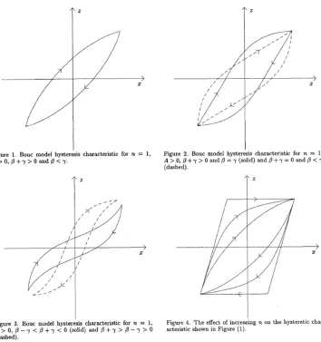
2.1 Various shapes achieved by tuning the Bouc-Wen model parameters, with fixed constraints of A>0 and n=1, from[8]. With one expression, Bouc-Wen model is able to generate different paths for tensile and compressive travels. The relationship betweenβ andγis different for each figure. . . 8 2.2 Classification of Bouc-Wen models, from Ikhouane et al[9]. Passivity of Class I Bouc-Wen

model was demonstrated in their research. The constraints were used in this thesis project. 9 2.3 Illustration of Bouc-Wen hysteretic model for bushing[7], consisting of simple stiffness,

damping and hysteresis modules . . . 9 2.4 Spencer MR damper model[7], with the extra state modeling the controllable hysteresis

change . . . 10 2.5 Ok, Yoo and Sohn bushing model[7], considered as the evolved Spencer model with

stiffness collaborating with Bouc-Wen expression . . . 11 2.6 A typical stiffness spline. There are only nine data points, meaning interpolation is

neces-sary. In the current simulation process, an estimated damping value will be assigned and used along with this spline to mimic the bushing behaviour. . . 12 3.1 Illustration of the five modules in the Advanced Bushing Model (ABM). The transfer

func-tion module is opfunc-tional and can be turned off if frequency response is not a major concern. 17 4.1 Hydraulic Tester of ARDC MTS Elastomer Test System. Direction of the tested elastomer

has to be positioned vertically because the only active axis is z-axis. Additional fixture design may apply for elastomer with irregular shape, such as the hydro-mount shown in the picture. . . 20 5.1 Fitting process of the ABM, from_[19_]. Users will decide whether the transfer function

(13)

5.2 Illustration of MATLAB shaker concept, from[19]. X_fandX_estand for the coordinates of frame-side or engine-side joint of the powertrain mount (X_f1for LHS,X_f2for RHS, andX_f3

for torque strut on the vehicle PF), and the input displacement will be applied onX_f. X

vectors are assumed to move along with the same coordinate system of powertrain. . . 33 5.3 Illustration of MotionView virtual shaker. Note that the hinge had been added (the purple

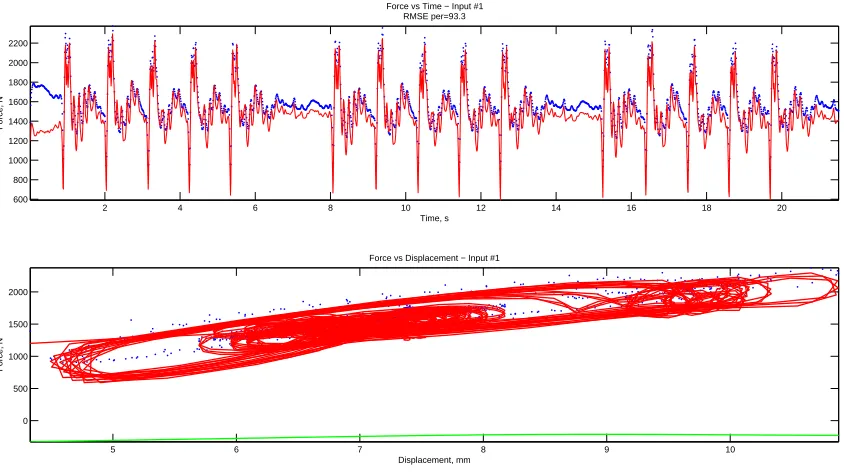
circular plate in lower right view). Because fitted ABM mounts were just in z-direction, the standard MotionView bushing model was used to model rotational as well as x and y-axis translational properties. . . 34 6.1 PF suspension bushing, with void and solid direction marked out . . . 35 6.2 PF Rubber Solid FDT 0 mm±4 mm 1 – 20 Hz. Target forces are in blue and simulated

forces are in red, and the stiffness polynomial in green (will be the same for all MATLAB plots) . . . 36 6.3 PF Rubber Void FDT 0 mm±3 mm 1 – 20 Hz. Stiffness polynomial matches well with the

general curvature. . . 38 6.4 PF Rubber Void RSIT 50% profile. Both force magnitude and hysteresis match well with

the test. . . 39 6.5 PF Rubber Void RSIT 80% profile. The stiffness polynomial tends to over-estimate the

force when exceeding the fitted region. . . 40 6.6 PF Hydraulic powertrain mounts, LHS(2) and RHS(3), and the chamber design(4). The

z-direction(1) was tested for each mount. . . 41 6.7 Sample of hydro-mount testing fixture, as the tester can only produce vertical motion. . . 41 6.8 PF LHSz SSIT 0.001 – 25 Hz 5 mm±1 mm, TF module only. Transient slopes are visible

for both tested and simulated force. . . 42 6.9 PF LHSz FDT 5.5 mm±6 mm 1 – 10 Hz. The stiffness polynomial does not follow the

central line in the hysteresis loop, because of the extra stiffness from transfer function. . . 43 6.10 PF LHSz FDT 5.5 mm±6 mm 10 – 20 Hz. Simulated force loops are visibly broader and

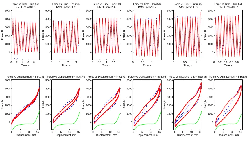
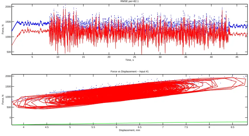
separate from test loops as frequency increases. . . 44 6.11 PF LHSz RSIT profile #1 at 2 mm initial offset. Although the overall shape looks fine,

insufficient stiffness causes static offset along the full travel. . . 45 6.12 PF LHSz RSIT profile #1 at 4.5 mm initial offset. RMSE fitness starts to increase as the

initial compression increases. . . 45 6.13 PF LHSz RSIT profile #1 at 7 mm offset. The overall fitness is near perfect. . . 46 6.14 PF LHSz RSIT profile #1 at 9 mm offset. Over-bending starts to show as the input

(14)

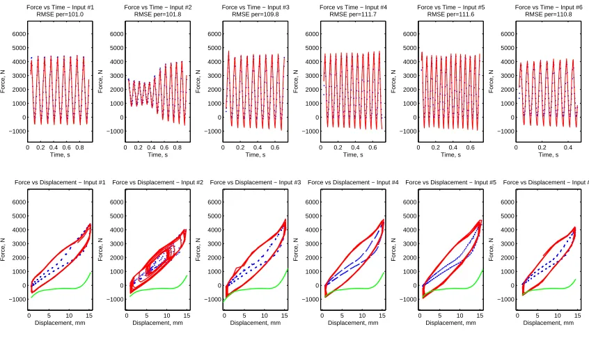
6.15 PF LHSz RSIT profile #2 at 2 mm offset. The ABM has no issue with capturing high-frequency motion contained by profile #2; However, the insufficient stiffness will still cause error. . . 47 6.16 PF LHSz RSIT profile #2 at 4.8 mm offset. Similar to results of profile #1, RMSE fitness

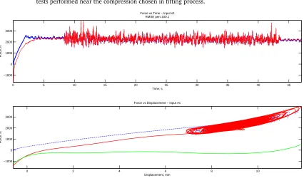
starts to increase as the initial compression increases. . . 47 6.17 PF LHSz RSIT profile #2 at 6.8 mm offset. Results are near perfect for tests performed

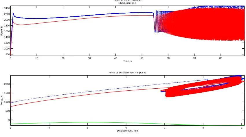
near the compression chosen in fitting process. . . 48 6.18 PF LHSz RSIT profile #2 at 9 mm offset. Output force becomes pointed as the displacement

leaves the fitted region. Static offset is not obvious. . . 48 6.19 PF LHSz SSIT 0.001 – 25 Hz 2 mm±1 mm. Despite the static offset, it is very distinct

that the transfer function can regulate the simulated force, making it constant in higher frequencies. Both curves are not identical, as the objective function itself does not include any frequency bias. . . 49 6.20 PF LHSz SSIT 0.001 – 25 Hz 5 mm±1 mm. As the compression increases, the static offset

shrinks accordingly, with the general response maintained. Note that this event was used for the TF fitting as well, so it shows the interference of extra stiffness from the TF module. 49 6.21 PF LHSz SSIT 0.001 – 25 Hz 8 mm±1 mm. Static offset becomes minor compared with

other compression magnitudes. . . 50 6.22 PF RHSz SSIT 0.001 – 25Hz 7 mm±1 mm, TF module only. The RMSE fitness is perfect,

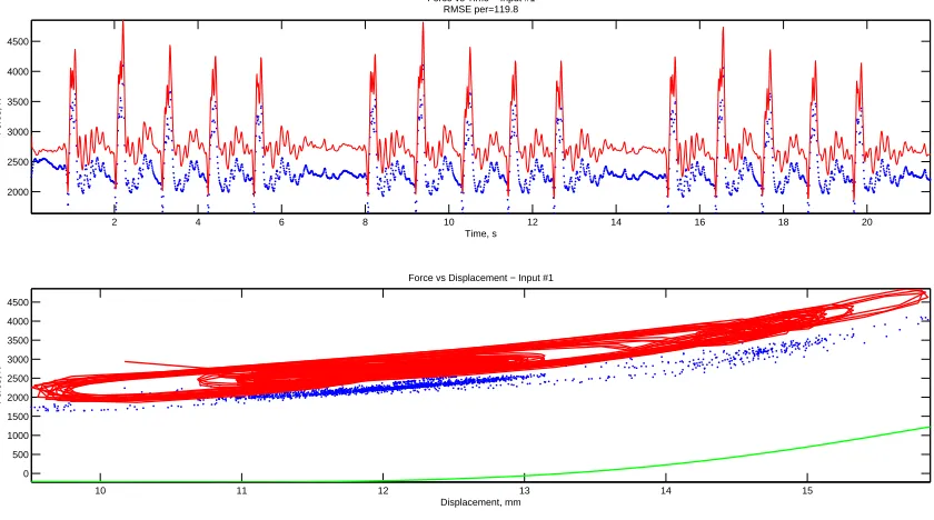
although two curves are not identical. . . 51 6.23 PF RHSz FDT 8 mm±7.5 mm 1 – 10 Hz. Hysteresis loops of the RHSz are heavily pinched

and pointed in the low compression region, making it difficult for the ABM to capture the general shape. . . 51 6.24 PF RHSz FDT 8 mm±7.5 mm 10 – 20 Hz. Test loops maintain near constant while the

simulated results get broader as the frequency increases. Some extra data points show that the controller on the test system was trying to regulate the displacement input to balance between the commanded displacement and frequency. . . 52 6.25 PF RHSz RSIT profile #1 at 3 mm initial offset. Because of the distorted stiffness

polyno-mial, static offset is quite large in low compression region. . . 53 6.26 PF RHSz RSIT profile #1 at 6 mm initial offset. Fitness increases along with further

com-pression. . . 53 6.27 PF RHSz RSIT profile #1 at 9 mm initial offset. The static offset behaves as an additional

increase to the measured data for RHSz simulation. Hysteresis loop is also broader than tested result. . . 54 6.28 PF RHSz RSIT profile #1 at 12 mm initial offset. Force starts to be pointed for high

(15)

6.29 PF RHSz RSIT profile #2 at 3 mm initial offset. Situation is similar to the profile #1 result at the same compression, with distinct offset and broad simulated hysteresis loop. . . 55 6.30 PF RHSz RSIT profile #2 at 6 mm initial offset. Simulated hysteresis loop is wide enough

to cover the test result, regardless of the static offset. . . 55 6.31 PF RHSz RSIT profile #2 at 9 mm initial offset. Best fitness among the same batch of events. 56 6.32 PF RHSz RSIT profile #2 at 12 mm initial offset. The overshoot offset pushes the travel

out of the fitted region, making the forces pointed. . . 56 6.33 PF RHSz SSIT 0.001 – 25 Hz 3 mm±1 mm. Transfer function still regulates the output

in similar shape as the tested curves, although the static offset cannot be eliminated. . . . 57 6.34 PF RHSz SSIT 0.001 – 25Hz 7 mm±1 mm. The same event was used for fitting

perspec-tive. The current result becomes worse due to distorted stiffness polynomial. . . 57 6.35 PF RHSz SSIT 0.001 – 25Hz 11 mm±1 mm. Considering the existing offset, this event

become the best fitting as it almost eliminate the effect. . . 58 6.36 Load comparison of tested and simulated result of MATLAB shaker, in CPG010 event.

CPG010 is a major event in damage calculation, due to its mixed road conditions. It is usually used as the calibration event in virtual shaker calibration. Simulated forces are generally smaller than tested data in the plots. . . 59 6.37 Zoomed in load comparison of tested and simulated result of MATLAB shaker at six time

intervals, in CPG010 event. Generally, the simulated forces follow the trend of the mea-sured results. The fitness becomes worse at some peaks and valleys, affecting the damage calculation. . . 60 6.38 Load comparison of tested and simulated result of MotionView shaker, in CPG010 event.

Peaks are generally mismatched from simulated force, and the damage would be reduced accordingly. . . 61 6.39 Zoomed in load comparison of tested and simulated result of MotionView shaker at six time

intervals, in CPG010 event. From the comparison, it is fair to say that most of the vertical motion has been reproduced. However, the magnitudes of the simulated and measured forces still do not perfectly match. Some instability from the simulated results can be seen in the last time interval. It is possible to eliminate the instability by tuning the MotionView solver. . . 62 7.1 Activated damping magnification according to velocities in the void direction. Large

(16)

7.2 Hysteresis loop comparison, with or without nonlinear damping. Compared with the test result (blue), hysteresis loop with nonlinear damping (red) is visibly broader than that without the nonlinear damping (green), under the 1 Hz FDT event input. Fitness is also improved in this way. . . 65 7.3 Activated damping magnification according to velocities on RHSz. Compared with the the

same plot for a rubber bushing, the shape is more pointed in the low velocity region. The magnification gets reduced in medium to high velocity region. . . 68 7.4 Inertia force depending on displacement, from the FDT fitting event on RHSz.

Regard-less of sudden accelerations generated from controller, forces from the mass module are concentrated below 100 N, and considered as minor. . . 68 7.5 Insufficient loads on both LHS and RHS mounts during the same time period. This would

suggest that the simulated motion failed to reach the desired locations on both mounts, which can be related to both the fitness of the ABM and the uncertainty in physical prop-erties of the powertrain. . . 71 B.1 Load comparison of tested and simulated result of MATLAB shaker, in CPG08U event. The

general trends in tested and simulated curves are the same, meaning most of the motions have been reproduced by the virtual shaker. Simulated curves miss some peaks and valleys, and are thinner than tested results. This could affect the damage comparison. . . 81 B.2 Zoomed in load comparison of tested and simulated result of MATLAB shaker at six time

intervals, in CPG08U event. Some differences can be spotted on simulated results of LHSz and RHSz, meaning the motion reproduction was possibly incorrect for certain region. . . 82 B.3 Load comparison of tested and simulated result of MATLAB shaker, in CPG021 event.

Sim-ulated forces on RHSz are larger than tested forces near 150s mark, which could be a possible source of large damage. . . 82 B.4 Zoomed in load comparison of tested and simulated result of MATLAB shaker at six time

intervals, in CPG021 event. The overall fitness in LHSz is fine, while the simulated results in RHSz are generally larger than tested results. . . 83 B.5 Load comparison of tested and simulated result of MotionView shaker, in CPG03A event.

Even without the mass module, some numerical noises will accumulate and becomes vis-ible near the end of the simulation. General fitness is still acceptable. . . 83 B.6 Zoomed in load comparison of tested and simulated result of MotionView shaker at six

(17)

B.7 Load comparison of tested and simulated result of MotionView shaker, in CPG04P event. Simulated forces in several peaks are larger than tested results, which would increase the damage. . . 84 B.8 Zoomed in load comparison of tested and simulated result of MotionView shaker at six

time intervals, in CPG04P event. The general fitness in large magnitude is fine. In small magnitude, the load change is mainly due to the vibration of the powertrain, that is im-possible to be reproduced using the data collected on chassis side. Thus the ABM mounts cannot reproduce such loads as well. . . 85 C.1 Torque strut on vehicle PF. As can be seen, the design of the torque strut combines the

factors of void and solid direction on conventional rubber bushing. The main functionality presents on x-axis as shown. . . 86 C.2 Stiffness splines of LHS mount. Damping values used were 1.5, 1.5 and 2.5 Ns/mm for x,

y and z-directions. Large slopes on both ends will provide sufficient stiffness to push the powertrain back into the effective region of the splines in the simulation. As can be seen, most of the efforts were applied in determining the z-directional stiffness, with most data points in returns. This is because vertical motion will generate the majority of the damages on the mounts, thus it is necessary to have a relatively fine expression on z-direction. . . . 87 C.3 Stiffness splines of RHS mount. Damping values used were 1.5, 1.5 and 1.5 Ns_/mm for

x, y and z-directions. Because the weight distribution on each mount is not even, plus the tolerances of motion are different, LHS and RHS will have individual stiffness and damping profiles. Despite this, some similarities in stiffness splines still present on z-directions of both LHS and RHS mounts. . . 87 C.4 Stiffness splines of torque strut. Damping values used were 2.5, 1 and 1 Ns/mm for x,

y and z-directions. The importance of the x-direction on torque strut equals to that of z-direction on LHS or RHS mount. This is also the reason why it is necessary to model the torque strut and joint in virtual shaker. Unfortunately, no data were found regarding the stiffness splines on y and z-directions of torque strut. They were replaced by a piece of artificial spline, applied twice on both directions. . . 88 D.1 Flow chart of drive file generation procedure using MATLAB, developed by X. Yang, S. Li,

(18)

List of Abbreviations

Abbreviation Meaning

ABM Advanced Bushing Model ANN Artificial Neural Network

ARDC Automotive Research & Development Centre BIBO Bounded Input-Bounded Output

CAE Computer-Aided Engineering CM Center of Mass

CPG Chelsea Proving Ground CR Center of Rotation CSE Control State Equation FDT Full-travel Dynamic Test GA Genetic Algorithm GSE General State Equation LHS Left-Hand Side

LTI Linear Time-Invariant MBD Multibody Dynamics MR Magneto-Rheological MTS MTS Systems Corporation NVH Noise, Vibration and Harshness ODE Ordinary Differential Equation PC Personal Computer

(19)

Nomenclature

Label Description

A,n,β, andγ Parameters of the Bouc-Wen hysteretic model

a₁toa₃ Coefficients of the denominator of the transfer function

b₁tob₄ Coefficients of the nominator of the transfer function

c Linear damping

c_nl Nonlinear damping ratio

c₀,C_d

1, andCd2 Parameters of the nonlinear damping ratio F_BW Force output from the Bouc-Wen model

F_damping Force output from the damping

F_mass Force output from the inertia mass

F_measured Measured force

f_nl(x) Nonlinear stiffness function

F_simulated Simulated force

F_stiffness Force output from the stiffness

F_tf Force output from the transfer function

k Linear stiffness

k₁tok₈ Parameters of the seventh-order stiffness polynomial

m Inertia mass ¨

x Input acceleration ˙

x Input velocity

x Input displacement

Y(x) Output force of the transfer function

z Bouc-Wen hysteretic displacement

(20)

Chapter 1

Introduction

1.1 Motivation

As a result of the rapid development taking place in computing technology, virtual simulation has become widely accepted in the engineering field, in order to reduce the time and cost in product development. Following this trend, increasing the quality of the simulation is highly focused, and the reliability of the simulated results depends directly on the accuracy of the virtual model representing physical system. However, not all virtual models available in the market meet all the demands from industry. This is when the virtual tool developers step in, to tailor custom codes and scripts that fit the special needs of the client.

(21)

usually built in the frequency domain, and cannot easily be exported for MATLAB simulation because of no access to the source code. The objective of this exercise is to provide a bushing model for the MATLAB shaker codes, while also exploring the ability to improve the modeling accuracy in the time domain.

1.2 Research Objectives

There were three primary goals established at the beginning of the project.

The first goal is that the proposed bushing model must be able to handle common phenomena present in real bushings. Three common phenomena are nonlinearity, asymmetry and hysteresis, and these are due to the certain purposes the bushing has to serve. So normally, a mature bushing model will cover these aspects, and most available bushing models are in this category.

The second goal is that the proposed bushing model can accommodate the specialty of hydraulic mounts, or hydro-mounts in abbreviation. With the hydraulic chamber inside, this type of mount can alter the dynamic stiffness as a function of frequency. Modeling of such a mount is always difficult, even for industrial software, but it was expected at least to provide this option for users of the proposed bushing model.

The third and the last goal is that the bushing model should not only be able to simulate with the virtual shaker table in MATLAB, but also be used by other commercial software. This would benefit the validation stage of the MATLAB shaker with the test-collected results, and can also extend the usage of this model. In this way, the proposed bushing model could replace the existing bushing models already in use for the convenience of the users in company.

1.3 Outline of Chapters

In this part, brief descriptions of each chapter will be given, to help in realizing the structure of this thesis. Chapter 1 is the introduction and the current chapter. This chapter mainly describes the motivation and objectives behind the thesis project, as well as the outlines of each chapter.

(22)

the thesis project will be reviewed. Previous works will be quoted and explained briefly. The chapter demonstrates the combination of many theoretical ideas into various models.

Chapter 3 is the detailed presentation of the proposed bushing model, the Advanced Bushing Model (ABM), its principles, and its functionality. Each module of the ABM will be explained with its purpose, equations, and related thoughts.

Chapter 4 describes the data collection for the proposed bushing model. The success of this model relied heavily on the ARDC MTS Elastomer Test System. General information regarding the system setup been given, and different types of test procedures requested for bushing model parameterization are also listed.

Chapter 5 reveals the coding highlights in the proposed bushing model. Some important considera-tions during the coding process will be discussed. A complete listing of the scripts is given in[1].

Chapter 6 presents the performance evaluation of the proposed bushing model. The two main topics in this chapter are validation and application. The proposed bushing model will be evaluated under various of conditions, and used with the virtual shaker table to see whether it will be able to reproduce the powertrain mount loads and damages.

(23)

Chapter 2

Background Review

There is a Chinese proverb: "By reviewing the past, one gains new knowledge." Sparks of innovation are usually based on the great works done by pioneers. This thesis project also builds on a number of theories and recommendations from early researchers. Their contributions will be emphasized in this chapter.

2.1 Bushing Types and Properties

The bushing is a widely used connection between two bodies of a mechanical system. It acts as an energy absorber to reduce vibration in the motion. A sample of its application is the suspension bushing of a vehicle, placed between two metal bodies in the system. The most common type of bushing is the rubber bushing. This type of bushing is made of synthetic rubber, providing adequate stiffness and damping rate for the design criteria. Occasionally the rubber structure will be partially hollowed to generate nonlinear stiffness and soften the damping rate.

(24)

In durability analysis, both types of bushing present similarities. Their plots of stiffness along the travel are usually nonlinear, with asymmetric travels in the extensional and compressive directions. In force-displacement diagrams they also form a hysteresis loop, a phenomenon that means the output de-pends on both current and previous inputs. There is also a major difference between these two bushings. Because of its NVH control purpose, the dynamic stiffness of the hydro-mount is frequency dependent, meaning the response plot in frequency domain will peak at a certain frequency. This frequency is usually high compared with that of body motion.

In bushing modeling history, there are numerous models accommodating some of these properties proposed by previous researchers. Most of them will include common linear stiffness and damping terms, as well as some methods for specific considerations. These methods will be discussed separately in following sections.

2.2 Linear Models - Transfer Function

The transfer function (TF) is a method of expressing the relationship between input and output of a linear time-invariant (LTI) system. The transfer function comes from the linear differential equation describing the same system. For example, a second-order linear system in time domain can be expressed as:

a¨y+b˙y+c y=f(t) (2.1) By applying the Laplace transformation, both the input signal f(t)and the output signaly(t)become:

L(f(t)) =F(s)

L(y(t)) =Y(s)

(2.2) Then the original equation can be written as:

(as2+bs+c)Y(s) =F(s) (2.3) Defining the transfer functionG(s)as the fraction of the output over input signal in the Laplace domain, it can be expressed as:

G(s) = Y(s) F(s)=

1

as2+_bs+_c (2.4)

(25)

longer unity for such a transfer function. These systems are said to containnumerator dynamics. For more details regarding to the transfer function, refer to[2], Chapter 8.

The immediate application of the transfer function in linear systems is the study of the frequency response. This is because the whole system is now described using the generalized frequencys rather than timet. There are many approaches to the frequency domain analysis through the transfer function, including determining poles and zeros [3]of the system. Considering the transfer function G(s) is a fraction of two polynomial functionsN(s)andD(s):

G(s) = N(s) D(s)=K

(s−z₁)(s−z₂)...(s−z_m₋₁)(s−z_m)

(s−p₁)(s−p₂)...₍s−p_n₋₁)(s−p_n) (2.5)

The poles will be the values ofs making the denominator zero, and the zeros will be the values ofs

resulting in a numerator of zero. In other words, poles indicate the system response of infinity and zeros represent zero response. Thus, it is important to calculate poles and zeros for the stability analysis.

Other than that, poles and zeros also introduce a concept categorizing transfer functions. Ifmand

nare the same for the expression above, both numerator and denominator will have the same order of

s. By definition, a transfer function in which the order of the numerator is less than or equal to that of denominator can be called apropertransfer function. Astrictly propertransfer function, more commonly seen, has a lower order numerator than denominator. Given more flexibility, the proper transfer function could be more generally useful.

(26)

compo-nent may not contribute significantly to fatigue in the durability test, as most of the damage in this test is from high amplitude travel in relatively low frequencies according to experts with practical experience.

2.3 Hysteresis and Bouc-Wen Hysteretic Model

Hysteresis is a nonlinear, history-dependent phenomenon that is widely seen in different fields and sys-tems. Generally, when using a periodic input, a looping graph will be witnessed when plotting the output versus input of a hysteretic system. Between the output and input of a hysteretic system, there are a num-ber of internal states. For bushings, hysteresis acts along with the motion-induced restoring force and energy dissipation. It depends not only on the current, but also previous displacement and velocity. Since the hysteresis is rate dependent, sometimes it is also referred as hysteretic damping.

Because the formation of the hysteresis can be different between systems, there are a number of models addressing this phenomenon. In bushing modeling, one popular model is the Bouc-Wen hysteresis model. This model was initially introduced as the Bouc model by Bouc in 1971[5]. It was revised by Wen in 1976[5], when it was given in the current form[6]:

˙

z=−γ|x˙|z|z|n−1₋_β_x_˙_|_z_|n₊_A_˙_x _(2.6)

This expression can be rewritten in another form[7], which is used in this thesis project, as: ˙

z=x˙{A−[γ+βsgn(˙x)sgn(z)](|z|n₎

} (2.7)

(27)

Figure 2.1:Various shapes achieved by tuning the Bouc-Wen model parameters, with fixed constraints of A>0 and n=1, from[8]. With one expression, Bouc-Wen model is able to generate different paths for tensile and compressive travels. The relationship betweenβandγis different for each figure.

Since the solution of the differential equation is the history of the hysteretic displacementz, another parameterαcan multiplyzas a weighting factor, when calculating the restoration force from hysteresis. This factor is discussed in the section 2.4, which deals with the applications of Bouc-Wen model.

(28)

apply when the model is used to represent a physical system, i.e. a bushing for this thesis research.

Figure 2.2: Classification of Bouc-Wen models, from Ikhouane et al[9]. Passivity of Class I Bouc-Wen model was demonstrated in their research. The constraints were used in this thesis project.

2.4 Models with Bouc-Wen Hysteresis

There are several existing models using the Bouc-Wen hysteretic expression. These models were not all specifically for bushing modeling, but other elastomers such as dampers. Ranking by complexity, here are some brief descriptions of three practical models in connection modeling, according to[7].

Bouc-Wen hysteretic model

This model is a basic model implementing the Bouc-Wen hysteresis expression. It consists of a linear stiffness, a linear damping and a Bouc-Wen component. All of the nonlinearity in this model relies on the Bouc-Wen expression. It can be used for bushings, or for magneto-rheological dampers as Spencer

[6]introduced.

(29)

The force out of this model can be expressed as:

F =k₀x+c₀˙x+αz (2.8)

Spencer magneto-rheological(MR) damper model

After studying the original Bouc-Wen hysteretic model in a), Spencer et al[6]proposed their model, which is especially applied for magneto-rheological (MR) dampers. In addition to the original Bouc-Wen model, Spencer introduces an internal state yin the damping term, with extra linear stiffness and damping. This sophisticated model reflects the controllable damping feature in MR dampers.

Figure 2.4: Spencer MR damper model[7], with the extra state modeling the con-trollable hysteresis change

The force out of this model can be expressed as:

F=k₀x+c₀˙y

c₀˙y=c₁(˙x₋˙y) +k₁(x₋y) +αz

(2.9)

Ok, Yoo and Sohn bushing model

(30)

Figure 2.5:Ok, Yoo and Sohn bushing model[7], considered as the evolved Spencer model with stiffness collaborating with Bouc-Wen expression

The force expression for this model is:

F=k₀y+c₀w˙

c₀w˙=c₂(˙x₋w˙) +k₂(x₋w) +α2z₂ k₀y=c₁(˙x−y˙) +k₁(x−y) +α1z₁

(2.10)

2.5 Stiffness Effect

Stiffness describes the resistance to the deformation of an object. It can also be referred to rigidity. Stiffness varies as a function of material and structure. On rubber bushings, stiffness provides force according to the displacement, which is commonly expressed as:

F=k x (2.11) Herekis the stiffness,xis the amount of displacement andF is the force generated. Within a reasonable range, many of the stiffnesses in a mechanical system can be modeled as linear stiffness, where the force generated is linearly proportional to the deformation. This is especially useful when using linearization to analyze a system. When the stiffness is used to connect the internal states within a model, it can also control the contribution of this internal state, as the output of the internal state will be suppressed by the stiffness.

(31)

fitting is needed to add the information between sample points. In a dynamic test, the displacement-force plot usually presents a loop, and the stiffness is viewed as the central line of the plot. If the loop is not given, an estimated value of linear damping will be assigned to mimic the shape.

−15 −10 −5 0 5 10 15

−5000 −4000 −3000 −2000 −1000 0 1000 2000 3000 4000 5000

Displacement,mm

Force, N

Stiffness Spline

Figure 2.6:A typical stiffness spline. There are only nine data points, meaning inter-polation is necessary. In the current simulation process, an estimated damping value will be assigned and used along with this spline to mimic the bushing behaviour.

2.6 Viscous Damping Effect

Damping is observed as the reduction of the oscillation in an oscillatory system. It dissipates energy during the process. Damping is rate dependent, meaning it is related to the velocity in a mechanical system. This can be expressed as:

F=c˙x (2.12) Herecis the damping ratio, ˙x is the velocity andF is the force. When modeling a system, usuallycis assumed to be constant for linear damping. Consider the equation of motion of a spring-mass-damper system:

F=m¨x+c˙x+k x (2.13) When massmand stiffnesskare constant, it makes the solution nice if the damping ratiocis also constant. In reality, most of the damping effects are nonlinear. Damping caused by the viscosity is categorized as viscous damping. It comes from the internal shear and tensile stress under deformation. For a rubber bushing, since the viscosity of rubber varies with temperature, properties under room temperature are commonly used. To determine the damping effect, a dynamic test is performed, and is subtracted from the static test result. The damping test data is a combination of viscous and hysteretic damping effects.

(32)

that the damping rate could be nonlinear for better characterization. This led to the consideration of a nonlinear damping expression. Although the expression used in this project is original, in later research a previous work using a similar expression for friction study was discovered, and will be presented. This model was proposed by Zhang et al in their nonlinear rate dependent friction research[10], and later applied in their work in modeling the slide guide in elevator systems[11]. The model is written as:

c(x˙) =c₀+c₁e−|˙x/c2|c3 _(2.14)

Herec₀,c₁,c₂andc₃are used to control the shape ofc(˙x). The resulting damping rate could be mono-increasing or mono-decreasing depending on the choice of parameters. In this thesis project, the nonlin-ear damping expression is restricted to compensate the performance when velocity is low. Details of the model will be discussed in Chapter 3.

2.7 Optimization Algorithms

In bushing modeling, because the defined model needs to be characterized using test data, proper op-timization methods are necessary in order to keep the simulated output as close to the test result as possible. There were two optimization methods, the genetic algorithm (GA), and Nelder-Mead method, applied on the proposed bushing model in different stages for the best performance.

The genetic algorithm is a method that mimics natural evolution. To initialize the solving process, an individual set of values is used as the initial guess of the parameters to be determined. A number of such individuals are used to form a population, and all individuals in the population will be evaluated in iterations. After each iteration, the genetic algorithm will select individuals as parents to generate new individuals, guiding the whole population towards the optimal solution. There are three main types of optimization that rule the evolution, from the Chapter 5 of Global Optimization Toolbox User’s Guide

[12].

• Selection rules select the individuals, called parents, that contribute to the population at the next generation.

(33)

The genetic algorithm is sometimes called a ‘shotgun’ method, due to its random initial value assign-ment and iterative approach. For a complex system, the genetic algorithm requires large computational power to balance between time cost and optimization depth. Because current computer workstations are commonly equipped with multiple cores, performance of the genetic algorithm can often be dramatically improved by using a parallel computing method.

Because the genetic algorithm can use a random set of initial values, it is a good method for starting the optimization of a system without initial guiding values. If a set of initial values has been given, there are other methods that can be used to refine the system. Among them, the Nelder-Mead method is the one that is frequently used in nonlinear optimization. This method was proposed by John Nelder and Roger Mead in 1965[13]. For an objective function withnvariables, the method will form a simplex withn+1 vertices inndimensions, e.g. a triangle in 2D-space or a tetrahedron in 3D-space. The simplex converges to minimize the objective function from the given initial points, and eventually returns the best fitted result. The algorithm is robust and less complicated, but the need in computational resource increases dramatically as the number of parameters grows. For modern computers, because it is a heuristic method working progressively, the Nelder-Mead method cannot be parallelly computed on a multi-core machine. However, it is still a mature algorithm with a relatively consistent results if the initial conditions are the same, and becomes a good complementary optimization method for the coarser genetic algorithm.

2.8 Neural Networks and Fuzzy Logic

Since the bushing can be treated as an input-output system, it is not absolutely necessary to specify the structure of the bushing model, while the model can be treated as a flexible model and represent the same relationship between input and output. This type of flexible model can be called a ‘black box’ model, as the knowledge of the structure within the model may not be necessary. Among those ‘black box’ models, neural networks and fuzzy logic are two popular models.

(34)

a new excitation is applied. By treating the displacement and force as an input-output couple, Johrendt and Frise[14]created an ANN rubber bushing model for virtual simulation, with success in improving the simulation accuracy.

(35)

Chapter 3

Proposed Bushing Model - the

Advanced Bushing Model (ABM)

3.1 Inspiration

After reviewing contents and information regarding bushing properties and Bouc-Wen hysteresis mod-eling, there are three basic components determined for a common bushing model, which are stiffness, damping and hysteresis components. The stiffness component must present nonlinearity in order to express the central line of the force-displacement loop, and must be flexible for different levels of non-linearity and asymmetry. This will also help reduce the difficulty in hysteresis fitting, as the Bouc-Wen expression alone is not well suited to express high levels of curvature. The linear damping was used initially, and later changed into nonlinear, based on observations during the fitting process.

Over the three common components, two extra components were applied on the proposed model. An inertia force was the first consideration, inspired by the bouncing fluid in the hydro-mount. The term was initially introduced to simply add some changes to the frequency response of the system, but later on it was found to contribute to the shape control in the fitting stage. The proper frequency dependency was configured by the other extra term, the transfer function. It is widely used in the analysis of linear systems.

(36)

mean-ing one or more components can be turned off in advance, and the fittmean-ing process will still continue.

3.2 Formation of the Advanced Bushing Model (ABM)

To begin, an illustration of the proposed bushing model, called Advanced Bushing Model (ABM), is shown as below. The ABM is a hybrid bushing model, in modular design. It consists of nonlinear stiffness, nonlinear damping, Bouc-Wen hysteresis and an optional transfer function module. A mass module is placed above all for inertia effects consideration.

Figure 3.1: Illustration of the five modules in the Advanced Bushing Model (ABM). The transfer function module is optional and can be turned off if frequency response is not a major concern.

And the force expression of the ABM is:

F=mx¨+c_nl˙x+f_nl(x) +αz+Y(x) (3.1) Thef_nlterm includes thek_nlin the illustration. Below are the explanations of each term:

m

: mass module that introduces an inertia effect. Its unit is 1000·kg if the input units are mm and s and the output unit is N. It provides the ABM with the ability to capture and regulate higher order motion than other existing models. To cooperate with other modules, there is no restriction on the sign. A negative sign will indicate the inertia force is opposite to the positive direction of the output force.

f

_nl

(

x

)

: nonlinear self-adaptive 7th order dynamic stiffness polynomial module, written as:

(37)

Herexis the input displacement andk₁tok₈are fitted polynomial parameters.

The f_nl(x)curve determines the magnitude-dependent force output of the fitted model. Normally, when plotting the force vs. displacement data of a bushing, the resulting graph is a loop. The stiffness curve is expected to be the central line of such a loop. Because of its description of the force-displacement relationship, the stiffness curve should be able to handle both nonlinearity and asymmetry, varying from bushing to bushing. This is also the reason why the module bears the name of ‘self-adaptive’, meaning it will be able to actively adapt its curvature to the best fit the result. Considering the ABM is usually fitted with dynamic test data, this curve can sometimes be called the ‘dynamic’ stiffness of the target bushing. However, since the modules collaborate with each other, the stiffness curve is no longer the central line when the extra stiffness from the transfer function module is included.

c

_{nl: nonlinear damping module, with its expression given as:} c_nl=c₀( Cd1

eCd2|x˙|+1) (3.3)

Herec₀,C_d1andC_d2are constants determined in fitting process, with constraints ofC_d1>0 andC_d2>0. The idea of having the damping rate as a variable with respect to the velocity was from observation. During the early stage of development, it was noticed that when performing multi-frequency fitting of a full-rubber bushing, the fitted hysteretic loop was much thinner at lower frequency (typically below 5Hz), when compared with that at higher frequency. This suggested that neither the Bouc-Wen model nor the linear damping work sufficiently below a certain frequency. Because frequency can be taken as a measurement of velocity in constant sine wave displacement inputs, the ideal solution would be to ‘patch’ the low velocity performance while keeping high velocity as is. This is what a reciprocal function can do, as a multiplier to the damping rate according to the current velocity. Giving more flexibility, theC_d1

decides the magnitude of magnification, and 1

eCd2|˙x| controls the rate of progression according to velocity

increase. Since bothC_d1 andC_d2 are positive, Cd1

eCd2|x˙| tends toward zero as velocity increases, andc0will

take over. To the best of author’s knowledge, no such function was used in any early bushing model. In later application, an accuracy increase was observed in the low velocity region, showing the benefit of having this nonlinear damping module in the ABM.

z

: Bouc-Wen hysteretic displacement in the hysteresis module, which has been explained in the previous section. Its expression can be recalled:

˙

(38)

This module contains the Bouc-Wen hysteretic model parameters, which areA, n,β andγ. The term

α is the magnifier of the z value. Consideringz is a type of displacement, α can be treated as the hysteretic stiffness. When using Bouc-Wen hysteresis for a physical system, its parameters have to meet the bounded-input-bounded-output (BIBO) and passivity requirement. These are defined as the initial constraints for fitting process.

Y

(

x

)

: optional proper transfer function module, but is used in state-space form: ˙

x=Ax+Bu Y(x) =C x+Du

(3.5) where theA,B,C,Dmatrices are from the realization of the third-order proper transfer function:

G(s) = b1s 3₊_b

2s2+b3s1+b4 s3+_a

1s2+a2s1+a3

(3.6) This module is designed especially for bushings where the frequency response is important, such as the hydro-mount. The transfer function is rewritten in the time domain, where its input is displacement and output is force. The reason for choosing a proper transfer function in this module is also from observa-tion. When using the sine sweep as the input displacement to the hydro-mount, the resulting force-time plot showed that under a constant magnitude input displacement, the output forces maintain constant amplitude at low frequency, then gradually increase in the medium frequency region and eventually be-come constant at a higher value in the high frequency region. A similar trend can be seen in the lead-lag compensator, which is described by a proper transfer function (refer to[2], pg. 327). To determine which order would be sufficient for the task, from second-order to fifth-order proper transfer functions were evaluated by simulation, and the third-order one met the balance between accuracy and efficiency. Thus, the default order of the transfer function is third-order.

(39)

Chapter 4

Bushing Data Collection

4.1 ARDC MTS Elastomer Test System

In the automotive industry, bushing tests often rely heavily on bushing manufacturers, due to their ne-cessity of demonstrating that the design goals are achieved. As the result, these data available for new bushing model development are incomplete. This is where the ARDC MTS Elastomer Test System plays an important role in this thesis project.

Figure 4.1: Hydraulic Tester of ARDC MTS Elastomer Test System. Direction of the tested elastomer has to be positioned vertically because the only active axis is z-axis. Additional fixture design may apply for elastomer with irregular shape, such as the hydro-mount shown in the picture.

(40)

test-ing. On the frame, there is a hydraulic actuator applying vertical load or displacement on the elastomer specimen (bushing in this project). The amount of load or displacement is generated by the hydraulic flow controlled by servovalves, which receive the converted signal from a closed-loop controller. The MTS FlexTest 40 is a PID controller that minimizes the error between desired and output value. The FlexTest 40 can control up to 4 channels. When running a single channel elastomer test, its sampling rate can reach up to 6144 Hz. However 512 Hz was chosen for bushing tests as a balance between accu-racy and data size. For pre-post processing, a desktop PC with MTS Series 793 Application Software is connected to the FlexTest 40 controller. With Series 793 applications, users are able to configure various types of bushing test inputs, including embedded cyclic load or displacement, plus user-defined input profiles. For more details about MTS assets used in the ARDC MTS Elastomer Test System, refer to[16]

[17] [18].

4.2 List of Bushing Test Procedures

(41)

Procedure Description Example Full-travel Dynamic Test

(FDT)

Constant sine wave inputs, start-ing at the midpoint and coverstart-ing the full travel of bushing. Fre-quencies of the sine wave cover as much of working frequency range as possible (at least from 1 to 10Hz)

Bushing with +4mm and -3mm travel: sine waves starting at

+0.5mm with amplitude of 3.5mm, at 1, 3, 5, 7, 9 and 10Hz if working frequency is not specified.

Random Signal Input Test (RSIT)

A piece of random displacement signal that lasts for 10-20 sec-onds is used as input displace-ment, starting at different offsets. Change the starting offset to dif-ferent locations and repeat the recording.

Displacement record from a real motion that a bushing sustained. To be used when validating deter-mined ABM parameters.

Sine Sweep Input Test (SSIT, Optional)

A sine sweep input starting from a very low frequency to a medium to high frequency with a low am-plitude. This test is necessary only if users want to include frequency response of a bushing (such as a hydro-mount) in the ABM using a transfer function.

Sine sweep test result of a hy-draulic powertrain mount, from 0.001Hz to 50Hz with 1mm ampli-tude, which is adequate to see the frequency response of the bush-ing.

Table 4.1:Types of necessary tests, from[19]

For each test, the following information were recorded, with the units consistent with Chrysler de-faults.

Name Description Example

Time Interval Second (s) To be recorded simultaneously when recording other information. Must be a fixed time interval (sampling rate).

Input Displacement Millimeter (mm) Describe the deflection applied on the bushing. Nor-mally, compressive deflection is noted in the+x direc-tion.

Output Force Newton (N) Measured force out of the bushing as the consequence of deflection. Normally, compressive force is noted in the+x direction.

(42)

(43)

Chapter 5

ABM in the MATLAB Environment

5.1 ABM Program Overview

As a numerical computation environment, MATLAB provides various functions and toolboxes for users to realize the desired functionality through programming. Similar to other user-made MATLAB programs, the main structure of the ABM program is in script format, i.e..mfiles. These scripts are either executable files or functions, depending on its individual role in the main program. Considering there are numerous works related to MATLAB programming, this thesis will focus more on the functionality of ABM rather than programming. The important functions will be mentioned. For a detailed script, refer to the script report[1].

The core of the ABM program are the ABM functions, mentioned in Chapter 3. The same functions will be used in different sequences according to the purpose of the individual script. As a program, the ABM consists of two main components. The first component is the ABM Fitting Tools. This component uses an optimization method to parameterize the ABM model. Most of the project time was dedicated to the improvement of fitting accuracy in this component. The second component is the ABM Executable. With the determined parameters, the ABM Executable can function as the virtual replacement of the target bushing in a simulation. Depending on the software environment the ABM is used with, two executables were made for MATLAB and Altair®_MotionView®_{simulation. There are also some common}

(44)

5.1.1 Common Files

These common files are custom functions that are not included in MATLAB packages used by Chrysler.

get_rms

This function calculates the root mean square error (RMSE) of the given data. RMSE is a common statistical measurement of data variation. In this function, the RMSE is expressed in terms of mean and standard deviation, as:

RM S E(x) =Æmean(x)2₊_std₍_x₎2 _(5.1)

wheremeanandstdare MATLAB inherent functions of calculating mean and standard deviation. The application of this function is typically to calculate and compare the RMSE of tested and simulated output force, giving users views whether the fitting is good, acceptable or poor.

ode2

(45)

tpdiff

This function differentiates the input data using 3-point first differentiation. The expressions of such differentiation with both boundaries are:

x_i₌₁= −x3+4x2−3x1

2h

x_i₌_n₍_n_≥₃₎= 3xn−4xn−1+xn−2

2h x_i₌_2,3,...,n₋₁= −xi−1+xi+1

2h

(5.2)

This is a basic differentiation calculation as well, maintaining consistency with another commercial soft-ware, named nCode, that is used by Chrysler for digital signal processing. Because nCode uses the algorithm for differentiation, both the ABM and the virtual shaker have to follow the method for the convenience of performance evaluation, making the result comparable between the two codes and with the same accuracy level.

5.1.2 ABM Fitting Tools

The ABM Fitting Tools are script packages used in the parameterization process of the ABM. The two main packages are the optimizer for the ABM and transfer function parameters.

ABM_optimizer

This is the main optimization script that calls the genetic algorithm (GA) function to tackle the penalty function of the specified optimizing event. Users will be able to start a new fitting event, or retrieve a saved event and refine the result. The saving behaviour of the ABM parameters is also controlled in this script. The parameters of the GA function can be tuned in this file. By default, the population size is 30 and the maximum number of generations is 100 when starting a new fitting. When refining the fitting, the maximum generation for a run increases to 200. In both cases, the termination value of the penalty function is defined to be 1e-12, in order to let the optimizer run to the maximum number of generations. To boost the optimization process, the parallel computing function will be automatically turned on if the Parallel Computing Toolbox in MATLAB can be found on the workstation.

ABM_penaltyfuncandABM_penaltyfunc_main

(46)

process, only data collected from FDT procedure are necessary. Pieces of information are assigned to the specific variables that can be recognized by the ABM optimizer, including the time step, displacement, force, etc. The input information will be passed fromABM_penaltyfunctoABM_penaltyfunc_main.

TheABM_penaltyfunc_maincontains the core functions of the ABM. As each function represents a module, these modules are fitted in sequence, following the logic shown below:

• If a transfer function module is called, the time history of input displacement will be used to cal-culate the transfer function forceF_tfin time history through the built-inlsimfunction. Otherwise,

F_tf=0 for the entire time.

• The input displacement and calculated velocity in the time history, along with a set of initial values assigned to Bouc-Wen parametersA,n,βandγby GA, are sent into Bouc-Wen function to generate the time history of hysteretic displacementz. The GA will also assign initial values for the magnifier

αin order to calculate the Bouc-Wen hysteretic forceF_BW

• The calculated input velocity in the time history are sent into the nonlinear damping module with the initial guess ofc₀,C_d1 andC_d2from the GA. The result is the damping forceF_damping.

• The calculated input acceleration in time history are sent into inertia module withmfrom the GA, to obtain the inertia forceF_mass

• The forces F_tf,F_BW, F_dampingandF_massare taken from the target force F_tested, and the magnitudes left are curve fitted by the seventh-order stiffness polynomial. The polynomial is then used to regenerate the stiffness force F_stiffnessby taking input displacement.

• The force out of the model now is the sum of forces from all the modules, F_simulated=F_tf+F_BW+ F_damping+F_mass+F_stiffness.

• The difference betweenF_simulatedandF_targetalong the entire time history is calculated as:

∆=

t∫end

tstart

(F_measured−F_simulated)2d t (5.3) This difference is to be minimized by the GA function, by refining the parameter selections. The process repeats until either termination condition is activated.

(47)

force, and display the percentage of similarity. For example, a value of 90 means the RMSE of the simulated force is a 90% match with that of the tested force in time domain.

To guarantee the bounded-input-bounded-output (BIBO) condition is met for the Bouc-Wen model, constraints ofA>0,γ+β >0 andγ−β≥0 are defined at the beginning of the script. To make sure the Bouc-Wen force follows the same positive direction as in the ABM,α >0 is included. Constraints for nonlinear damping, meaningc₀>0,Cd1>0 andCd2>0, are also defined. If any of these conditions is

void with the value assigned by the GA, the penalty function will be set to infinity, to force the GA to skip the choice.

During the development stage, these two files were in one script. To protect the source code, core functions were separated intoABM_penaltyfunc_mainand encrypted into.pcode, the protected format of.mfile. In this way, users will not be able to modify, reducing the risk of damaging the entire program.

ABM_BW_single

This function only contains the expression of the first-order Bouc-Wen hysteretic model. It becomes a stand-alone function because it is frequently called by the ODE solver.

ABM_RUN_penaltyfunc

The purpose of the script is to provide users ability to simulate the fitted model with other inputs. Its structure is the same as ABM_penaltyfunc_main, except all the parameters will be assigned by users instead of by the GA. To reduce the workload, only the fitting event name is required for the parameter import. The function will then automatically search for the.matfiles matching the description, which are the saved files fromABM_optimizer.

TF_optimizer

If the frequency dependency is a focus for the application, this package will be used with the SSIT data to determine the transfer function containing frequency response. TheTF_optimizeris the script starting the process. BecauseTF_optimizerstill uses the GA to initiate or refine the fitting, its structure is similar to the

(48)

accelerate the fitting process and present quality results. By mixed usage of the GA and the Nelder-Mead method in refinement, it is usually expected to have a set of acceptable parameters within two to three runs.

TF3c_detandTF3c_main

As the names suggest, the relationship between these two files is the same as that betweenABM_penaltyfunc

andABM_penaltyfunc_main. First,TF3c_detreads in the input file and passes the information toTF3c_main, where the third-order proper transfer function is deployed. Still, the GA will choose the initial guesses of the seven parameters, and the visualized results are force-time and force-displacement plots with RMSE ratio displayed. The MATLAB built-in functionlsim, which will quickly return the simulated result of a linear system, is used to accelerate the simulation process. The penalty function is the same as that in

ABM_penaltyfunc_main.

5.1.3 ABM Executable

These executables make the ABM fitted result available to other applications, mainly for the parallel virtual shaker project.

ABM_ss

TheABM_ssis a.mfunction that can be used in MATLAB. It is designed to be used with the MATLAB version of the virtual shaker table. By taking input displacement, velocity, acceleration and the internal state of the Bouc-Wen model, theABM_ssfunction uses ABM fitted results to calculate the output force along with the new internal state at the time point. It is designed in such way so that it can collaborate with the shaker script, which is essentially a set of equations of motion that needs to be solved by an ODE solver. By exchanging the internal state with the main shaker script, there is no need for a separate ODE solver specifically for ABM.

Because experienced users may want to tune the ABM performance, an extra correction factor ma-trix is introduce in the function. This mama-trix allows users to define the percentage of contribution from five modules in ABM, in sequence of mass, stiffness, damping, Bouc-Wen hysteretic and transfer func-tion force. For example, a [1;1;1;1;1]matrix means all modules have original functionalities, while

(49)

ABMsub.soandABM_xyz.mdl(For MotionView)

Altair®_HyperWorks®_MotionView®_{is a commercial multi-body dynamics solver used by Chrysler,}

con-sidered as typical in their work flow. To integrate the ABM into the commercial program, the only solution is to write a subroutine that can be called by the MotionView solver. Thus, theABM_sshas been rewritten into the General State Equation (GSE) format of MotionView, in the FORTRAN language. The script was then compiled using the MotionView library, and can be called through the Control State Equation (CSE) in a MotionView user-defined script. To reduce the difficulty, a subsystem calledABM_xyz.mdlwith the ABM on x, y and z translational directions is developed. Now users will only need to import the subsys-tem into the main MotionView model, connect the joints and insert the parameters, and start to simulate with the ABM in the MotionView environment.

5.2 Parameterization using ABM Fitting Tools

Prepared Data

ABMFT TF-optimizer

ABMFT ABM-optimizer

9 parameters 1 polynomial TF parameters

Fitted ABM

With TF Without TF

Figure 5.1: Fitting process of the ABM, from[19]. Users will decide whether the transfer function (TF) module is necessary for fitting in the beginning, as the transfer function parameters have to be included in the ABM-optimizer fitting if applicable.

Development of a Bushing Model for Vehicle Durability Simulation

Scholarship at UWindsor

Scholarship at UWindsor

Electronic Theses and Dissertations

Theses, Dissertations, and Major Papers

2014

Development of a Bushing Model for Vehicle Durability Simulation

Development of a Bushing Model for Vehicle Durability Simulation

Sida Li

Recommended Citation

Recommended Citation

FOR

V

EHICLE

D

URABILITY

S

IMULATION

by

Sida Li

A Thesis

Submitted to the Faculty of Graduate Studies

through the Department of

Mechanical, Automotive, & Materials Engineering

in Partial Fulfilment of the Requirements for

the Degree of Master of Applied Science at the

University of Windsor

Windsor, Ontario, Canada

2014

by

Sida Li

APPROVED BY

Dr. X. Chen

Department of Electrical and Computer Engineering

Dr. J. Johrendt

Department of Mechanical, Automotive, & Materials Engineering

Dr. B. Minaker, Advisor

Department of Mechanical, Automotive, & Materials Engineering

Declaration of Co-Authorship

Abstract

Acknowledgements

Contents

List of Tables

List of Figures

List of Abbreviations

Nomenclature

Chapter 1

Introduction

1.1

Motivation

1.2

Research Objectives

1.3

Outline of Chapters

Chapter 2

Background Review

2.1

Bushing Types and Properties

2.2

Linear Models - Transfer Function

2.3

Hysteresis and Bouc-Wen Hysteretic Model

2.4

Models with Bouc-Wen Hysteresis

2.5

Stiffness Effect

2.6

Viscous Damping Effect

2.7

Optimization Algorithms

2.8

Neural Networks and Fuzzy Logic

Chapter 3

Proposed Bushing Model - the

Advanced Bushing Model (ABM)

3.1

Inspiration

3.2

Formation of the Advanced Bushing Model (ABM)

m