ABSTRACT
MAI, ZIYI. Do Terms-of-Trade Shocks Affect Exchange Rate Regime Choice? (Under the direction of Dr. Asli Leblebicioglu.)
Classical studies on the exchange rate regime choice have investigated
factors like common border, colonial connect, trade, etc, but few look at the
impact of terms-of-trade on the choice of exchange rate regime. This paper
helps to explain the possible connection between shocks on terms-of-trade and
exchange rate choice. I use post Bretton-Woods sample (1980-2007) of
ninety-one countries to access if shocks on terms-of-trade would have a significant
effect on the choice of exchange rate regime using OLS and logistic regression.
The results show a statistically negative and significant effect of terms-of-trade
shocks on the choice of exchange rate regime, along with some factors that are
consistent with the previous studies. These results also suggest an economically
relevant role for terms-of-trade in the determination of exchange rate regime
choice since significant amount of world trade is conducted between countries
© Copyright 2011 by Ziyi Mai
Do Terms-of-Trade Shocks Affect Exchange Rate Regime Choice?
by Ziyi Mai
A thesis submitted to the Graduate Faculty of North Carolina State University
in partial fulfillment of the requirements for the Degree of
Master of Arts Economics
Raleigh, North Carolina 2011
APPROVED BY:
_________________________ __________________________ Asli Leblebicioglu Atsushi Inoue
Chair of Advisory Committee
BIOGRAPHY
The author was born in Guangzhou, China, 1983. He earned his Bachelor’s
degree in Economics and is interested in open economy, monetary policy and
international trade. He currently is a graduate student in economics at North
ACKNOWLEGEMENTS
I would like to thank Atsushi Inoue for his support regarding econometric
techniques used in this paper. I am especially grateful to Asli Leblebicioglu for
her patience and kindness to direct me to finish this paper on every step along
the way. I also benefited from helpful comments of Atsushi Inoue, Mark
TABLE OF CONTENTS
LIST OF TABLES ... v
LIST OF FIGURES ... vi
1. Introduction ... 1
2. Trends in Choice of Exchange Regime in Modern Era ... 2
3. Literature Review ... 6
3.1 Optimum Currency Area ... 6
3.2 Macroeconomic consideration on countries’ choice of exchange rate regime ...10
3.3 International Trade and Exchange Rate Regimes ... 12
3.4 The conventional debate over terms-of-trades shocks on exchange rate regime ...13
4. Empirical Analysis ...16
4.1 Hypothesis and Methodology ... 16
4.2 Data ... 20
4.3 Empirical results of Exchange Rate Regime Choice ... 22
5. Concluding Remarks ...25
REFERENCES ...27
APPENDIX ...34
LIST OF TABLES
LIST OF FIGURES
Figure 1. Frequency Distribution of Exchange Rate Regimes (in percent) .... 29 Figure 2. Real Exchange Rate Volatility (in percent per year) at Alternative
1. Introduction
Post Bretton-Wood era has seen a tremendous shift from the pervasive pegged
exchange rate to a wide variety of exchange rate regimes, including independent
floating, managed floating, crawling pegged etc. Furthermore, during the
modern era, many countries have switched from one type of exchange rate
regime to another and often have flipped back and forth another time or two. Since most of the countries in the world didn’t cast off the chain of gold
standard and had spent decades under the Bretton-Wood system, theories and
empirical studies about the choice of exchange regimes have not sprung up until
early 1980s. Conventional studies concerning what determines a country to
adopt fixed or floating exchange rate system have investigated a wide variety of
factors in different categories. Most of them have interpreted the reasons from
the monetary perspective and the need for more trade. This paper tries to
countries and time by providing empirical results, based on the traditional
studies.
In this paper, I specify terms-of-trade as a new factor that previous studies have
not paid enough attention to, based on the framework developed by Shambaugh
and Kevin (2010). I use a set of data including 91 countries, from 1980 to 2007
to operate both OLS and logistic regression. The results show evidence that
there is a negative connection between the positive shocks on terms-of-trade
and the likelihood on choosing fixed exchange rate regime and vice versa.
2. Trends in Choice of Exchange Regime in Modern Era
Exchange rate policy is just one facet of the country’s overall set of
macroeconomic policies, but an appropriate choice of exchange rate regime can
help the country meet particular macroeconomic goals. This section briefly
describes broad trends in exchange rate regimes based on de jure and de facto
categorization that can be divided into pegged, intermediate, and floating
In past decade there have been important developments in the choice of
exchange rate regimes across countries. For advance economies, the most
significant development was the adoption of irrevocably fixed exchange rates
and a common currency by the euro area countries in 1999 (Figure 1[a]). Since,
under European Exchange Rate Mechanism II, these countries’ currencies were
allowed to fluctuate within wide bands, they were previously classified as
having an intermediate exchange rate regime. Although the euro floats against
other currencies, countries adopting euro are classified as having a peg, both
because the empirical analysis uses country-level (rather than euro area)
statistics, and because it would be strange to treat the adoption of a common
currency as a move toward greater flexibility.
Among emerging market economies (Figure 1[b]), three trends are
discernible. First, consistent with the 1999 review1 and the bipolar prescription,
there is significant hollowing out of the intermediate regime category. Second,
since the 1999 review, the proportion of both de jure and de facto floating
exchange rate regimes has roughly doubled. However, contrary to the
1International Monetary Fund, 1999, “Exchange Rate Regime in an Increasingly Integrated World Economy”.
prescription in the 2003 review2, the proportion of de facto floating regimes has
fallen somewhat since 2003 (Figure 3). Third, there is significant divergence
between the de jure and de facto classifications. In a number of cases, the
central bank intervenes in the foreign exchange market without taking on the
formal commitment to the peg. This is reflected in a larger number of de facto
pegs than de jure pegs, and a larger number of de jure floats than de facto floats.
In developing countries, there has been no hollowing out of the (de jure or
de facto) intermediate regime category (Figure 1[c]). The proportion of de jure
pegs and de jure floats has also remained constant over the past decade (with a
slight increase in pegs and decrease in floats). And, as with emerging market
economies, there is significant divergence between de jure and de facto regimes.
The divergence between de jure commitments and de facto behavior,
evident in both emerging market and developing countries, nearly always
reflects cases where the central bank intervenes but does not commit to the
parity. The opposite case-taking on a de jure commitment but de facto not
defending the parity-is much rarer. Indeed, across the full sample, in more than
90 percent of cases where the exchange rate is de jure pegged it is also de facto
2International Monetary Fund, 2003, “Evolution and Performance of Exchange Rate Regimes”. The 2003 study
focused only on growth and inflation performance, replacing the de jure classification of regimes with the IMF’s de facto measure. It found out that the costs of pegged regimes for emerging market economies
pegged, but only in 50 percent of cases where the exchange rate de jure floats
does it also de facto float.
Together, these trends suggest that developing and emerging market
countries have only partially followed the advice of previous studies conducted
by International Monetary Fund. Thus, consistent with the 1999 review, there
has been some hollowing out of the middle; and, following the 2003 study,
more emerging market countries are de jure floating their exchange rates.
Contrary to the prescription of these two reviews, however, a large proportion
of developing and emerging market countries de facto peg their exchange
rates-intervening in the foreign exchange markets without taking on the formal
commitment to the peg. However as elaborated below, this may be the worst of
both worlds: providing neither the policy discipline nor credibility of a formal
peg nor the benefits of flexibility that a floating exchange rate affords. While
the inflation benefits of pegging accrue mainly to de jure peg (particularly in
emerging market countries), the costs in terms of susceptibility to crisis and
3. Literature Review
The past three decade has witnessed a great amount of fruitful thoughts
and theories concerning the factors that affect the choice of exchange rate
regimes. In this section, I lay out four kinds of framework that previous studies
have looked at on the matter that this paper is concerned. The first part is
optimum currency area, originally developed by Mundell in 1961. In the second
part I present some macroeconomic considerations that countries have to take
into account before governments decide which one should adopt. The third part
shows the indivisible importance between international trade and exchange rate
regimes. The last part throw out some conventional views on the relationship
between terms-of-trade shocks and exchange rate regime.
3.1 Optimum Currency Area
The nature of the exchange rate regime choice is different in the modern
era than in earlier times. The choice of whether to participate in the gold
standard was bound up with the choice of whether to be engaged in the broader
international monetary system. This had implications for international trade,
since participation in the gold standard was viewed as a way to foster trade, an
system (Flandreau 1996; Meissner, 2005). It also had implication for
international borrowing, since membership in the gold standard was a way to
ensure international investors of creditworthiness (Bordo and Kydland,1996).
For these reasons, and also because of limited enfranchisement and a view that
governments were not fully responsible for economic conditions, once
governments pegged to gold, they had a tendency to consistently maintain this
policy, through good times and bad times, up until World War II. After World
War II the Bretton Woods system of fixed exchange rates was also relatively
stable, with only a few cases of government opting out of the system and
allowing their currencies to float. Unlike the earlier gold standard period,
exchange rate regime stability in the Bretton Wood era was supported by
restrictions on international capital mobility which afforded countries some
scope for setting monetary policy despite participation in a fixed exchange rate
system.
As we have seen, the hallmark of the modern era has been a wide
heterogeneity in exchange rate experiences, even among countries at similar
levels of economic development. So the question of exchange rate regime
Woods periods, since it is not bound up with the broader question of whether to
be engaged in the global economy.
A central framework for accounting the relative gains and losses of a fixed
exchange rate system versus a flexible exchange rate is optimum currency area
(OCA) theory., originally formulated by Mundell(1961). Strictly speaking, this
theory focuses on the choices of a country to participate in a currency union, but
its insights can be used to interpret the relative desirability of a fixed exchange
rate as opposed to a floating exchange rate since the relevance of its main
principles do not differ if one considers a currency union or , instead, a fixed
exchange rate. The central idea of OCA theory is that a country should weigh
the microeconomic benefits of membership in a currency union (or fixed
exchange rate) against its macroeconomic costs. The microeconomic benefit is
the reduction in exchange rate uncertainty for trade with other members of the
currency union (or alternatively, with the base country and with other countries
that peg to the same base). The macroeconomic cost is abandoning autonomy of
monetary policy, which could otherwise be used to stabilize business cycles.
Counter to the microeconomic benefits indentified by OCA theory are the
macroeconomic costs of pegging a currency. OCA theory focuses on economic
transfers and labor mobility. However, it’s likely that these two features are not
especially relevant for many countries. Immigration restrictions in many
countries have tended to limit countercyclical movements of workers over the
past four decades. It may be the case that the single currency in Europe, for
example, is importantly supported by the relative ease with which citizens of
countries that are members of the European Union to work in other member
countries. The point is that in a cross-country analysis it may be difficult to
identify variables that are useful proxies for those things identified by Mundell
that make membership in a currency union more attractive by mitigating the
adverse consequences of abandoning an independent monetary policy.
One implication of OCA theory for the choice of a fixed exchange rate
versus a flexible exchange rate is that two countries benefit more from having a
fixed exchange rate if they trade more, or if there is a higher potential for trade
between them. Thus the level of trade with the base country ( or the potential
base country) should be positively correlated with the choice with the choice of
a fixed exchange rate.
OCA theory also points out that forgoing monetary autonomy is less of a
problem when there is a natural coherence in business cycles among members
more proximate, or that share a common border, have a higher degree of natural
coherence in their business cycles.
3.2 Macroeconomic consideration on countries’ choice of exchange rate regime The second theoretical framework that informs our understanding of the
choice of an exchange rate regime also focuses on macroeconomic
considerations. First, the policy trilemma points out the fact that, in the presence
of international capital mobility, a fixed exchange rate ties the hands of
monetary authorities. Therefore we might expect to see a greater tendency for a
country to have a fixed exchange rate when it has controls on international
capital flows, since this would allow some level of monetary autonomy, even
when there is a fixed exchange rate.
Second, it also points out that output is relatively more stable with a fixed
exchange rate rather than a flexible exchange rate if the shocks hitting an
economy are dominated by asset market disruptions rather than disruptions in
the goods market.
Third, if output under fixed exchange rate regime, as policy trilemma
points out, counties especially developing countries might be in favor of fixed
exchange rate regime to sustain the growth rate. Previous studies have shown
economies is higher under pegged and intermediate exchange rate regimes
compared to floating exchange rate regimes in terms of unconditional averages.
In emerging market and developing countries, growth rates do not differ
markedly between pegged and floating exchange rate regimes, while
intermediate regimes exhibit the highest output growth rates. (Ghosh,2009)
Four, exchange rate regime might become a useful weapon to counter
financial crises and stable the economy. Financial crises are a more extreme
form of volatility, which also leads to shock on terms-of-trade. Avoiding them
as possible is an essential goal of the exchange rate regime choice-important to
the individual country because of the economic and social costs of the crisis and
important to the rest of the system because of the risk of contagion. Empirical
Analysis (Bubula, Andrea, Inci Otker,2003) suggests that currency crises are
somewhat more common under intermediate regimes compared to pegged or
floating exchange rate regimes. In financially open developing or emerging
market economies, there is significantly higher likelihood of a financial crisis
under a pegged or an intermediate regime than under a floating exchange rate
3.3 International Trade and Exchange Rate Regimes
One of the key attributes of a stable system of exchange rates system is
that the exchange rate should facilitate the exchange of goods, services and
capital. By reducing exchange rate uncertainty, pegged exchange rate regimes
should lower the cost of cross-border transactions-particularly those that
involve long horizons, such as foreign direct investment, where the uncertainty
cannot be easily hedged (Werner,1970). A first question, therefore, is whether
less flexible exchange rate regimes indeed reduce real exchange rate
volatility-and over what horizon. From Figure 2, pegged volatility-and intermediate exchange rate
regimes exhibit lower real exchange rate volatility than floating regimes, with
the volatility decreasing in the length of the horizon. Even at a one-year horizon,
however, the volatility under floating regimes is close to twice the volatility
under pegged or intermediate regimes (Mussa, 1986). However at very long
horizons (four to five years), average volatility of the real exchange rate under
floating regimes is actually slightly lower than under intermediate
3.4 The conventional debate over terms-of-trades shocks on exchange rate regime
The choice of the exchange rate regime has always been an area of great
controversy and debate. The discussion has once again taken center stage in the
world. Milton Friedman (1953) argued that one of the most important
advantages of flexible regimes over fixed regimes is that they can smooth
adjustment to real shocks even in the presence of nominal rigidities. Ever since,
this has been one of the least disputed benefits attributed to fully flexible
exchange rate regimes. Subsequent to Friedman, many theories of the
international transmission of real shocks have confirmed the original intuition
that the short-run responses to terms-of-trade shocks should be different across
exchange-rate regimes.
Following the works of Robert A. Mundell (1968) and William Poole
(1970), many economists still believe that the relative merits of exchange rate
regimes depend on the nature of the shocks that buffet the economy. When
shocks come from the domestic money market, fixed regimes automatically
prevent them from affecting the real economy. In the event of a positive
demand shock, money supply increases as monetary authority buys foreign
unchanged. On the other hand, flexible regimes require income to fall so that
real money demand is reduced back to the unchanged level of real money
supply. Therefore, if these shocks predominate in the economy, this is an
argument in favor of fixed regimes.
However, when shocks are mostly real, floating exchange rate regimes are
in theory the more effective choice. Indeed, one of the most important benefits
commonly attributed to fully floating exchange rate regimes is that they allow
smooth adjustment to real shocks. When domestic prices are sticky and thus
change at best slowly in response to shocks, a negative real shock, as a fall in
export demand or an increase in import demand, leads to a depreciation of the
nominal exchange rate. This depreciation in the exchange rate, in turn, reduces
the relative price of tradable goods at precisely the moment when demand for
them has fallen and therefore partially offsets the effect of the negative shock.
Furthermore, the nominal depreciation increases the domestic price of the
export good exactly when foreign price has fallen, also helping the economy
have a smoother adjustment. That is, the exchange rate acts as an automatic
stabilizer in flexible regimes.
On the other hand, fixed regimes have to rely on the slow changes of
have to live with the effects of the negative shock. Moreover, the central bank
must prevent the currency depreciation that would otherwise occur by buying
domestic money with foreign currency. This is inherently a contractionary
action and induces an additional fall in employment. The long and painful
deflationary periods necessary to realign relative prices in the United Kingdom and in Argentina during the 1920’s and 1990’s, respectively, serve as a
reminder of the costs associated with a fixed nominal exchange rate.
A second channel through which floating regimes are able to smooth
shocks is the freedom they have to pursue an independent monetary policy. In
the presence of real negative shocks, governments would like to be able to
respond to alleviate the recession. Under flexible rates, the country can respond
by means of a monetary expansion. Under fixed rates, any injection of money
would imply an outflow of reserves and no effect on output.
In the developing world, flexible exchange rate regimes can insulate the
economy better from real disturbances (Broda, 2001). Floats have smoother real
output paths after terms-of-trade shocks. There also seems to be no fear of
floating in response to terms-of-trade shocks, since floats let their nominal
Furthermore, terms-of-trade shocks are inflationary in floats and deflationary in
pegs. (Aghion, Bacchetta and Banerjee, 2000)
4. Empirical Analysis
4.1 Hypothesis and Methodology
In this paper I am specifically interested in how the variations on
terms-of-trade affect the likelihood of the choice on exchange rate regimes. First as
convention I define terms-of-trade as the ratio of export prices to import prices,
presented as index numbers. Terms-of-trade indicate the purchasing power of a country’s exports in terms of the imports that they will buy. A rise in the
terms-of-trade index indicates an improvement in the terms of trade: one unit of
exports will buy more imports. In light of the theory developed by Friedman
(1953), a fall in the demand of export goods or an increase in the demand of
import goods, which is a real negative shock on terms-of-trade, will lead to
depreciation on nominal exchange rate. In order to maintain the peg under fixed
exchange rate regime, a central bank has to inject money into domestic market,
which increases the money supply and implicitly leads to inflation. This implies
probability that they will switch from fixed exchange rate regime to a floating
one. Thus the sign of coefficient on terms-of-trade is expected to be negative.
The other regressors I use in the model follow the framework formulated
by Shambaugh and Kevin (2010). Optimum currency area theory suggests that
countries with more potential to trade are more likely to have a pegged
exchange rate. For those countries with higher GDP per capita and larger
population, they have more potential to trade but tend to be more diversified
when they trade, and thus have fewer incentives to peg. For small countries
with high GDP per capita but with a small population have more incentive to
trade and are prone to peg their currencies to a base country. The effect of trade
on large countries that do not tend to peg would be likely to be set off by the
effect on small countries that have great incentive to peg. Since small countries
in this sample outnumber large countries, I expect the coefficient on GDP per
capita would be positively associated with the peg status. Following the
assumption that the exchange rate volatility significantly diminishes bilateral
trade (Cushman, 1983), those countries which want more trade are prone to peg
their currency to a base country to avoid the risk of exchange rate volatility.
Thus the coefficient on the percentage of trade over GDP is expected to be
exporters that have great incentive to peg their currencies. However, some
advanced countries like Norway and U.K. that have relatively higher oil rent
but in fact export less crude oil than those Middle East counties might tend to
offset the effect of this variable as a substitution. Therefore the coefficient of
the oil rent is expected to be ambiguous. The model is specified as following:
E(PSit)=β1ln(TOT)it+β2ln(GDP)it+β3GM2it+β4ln(OR)it+β5ln(TRADE)it+β6ln(PO
P)it+ β7(GOV)it+ηi+θt
PS is peg status where 1 indicates a country chooses fixed exchange rate system
and 0 indicates a country chooses floating exchange rate system. GDP is GDP
per capita. GM2 is the grow rate of qusi-money M2. OR represents the oil rent
measured by U.S. dollars. TRADE is the ratio of total trade over a country’s
GDP. POP is population take the first difference. GOV specifies the ratio of
government spending over GDP. η specifies courtiers fixed effect while θt
capture the year fixed effect. The model is armed with logistic regression as the
methodology, along with the regular Ordinary Least Square estimation as
comparison. The logistic model is a generalized linear model used for
prediction of the probability of occurrence of an event by fitting data to a logit
this empirical analysis is binary variable, in which 1 indicates choice of fixed
exchange rate regime and 0 for floating one. Also, the logit mode does lend
itself to a fixed effects treatment for the heterogeneity. The purpose of using
probability linear model is to provide a wider perspective with how much the
result is consistent with the one under logistic regression. The reason that I
prefer logistic regression instead of OLS as a more accurate way to measure the
impact of terms-of-trade is that logistic model is able to guarantee the
coefficients are between 0 and 1. I also add country fixed effect which captures
the factors that are time invariable such as languages and laws, and year fixed
effect that capture variables affecting all the countries at the same time such as
global price shocks.
I use a panel (time-series, cross sectional ) data set that includes de facto
exchange rate regimes constructed by Shambaugh (2004) over 28
years(1980-2007). Estimation is by a linear probability model(OLS) and logistic model.
The latter works seamlessly across panel, time-series, and cross-sectional data,
and it also offers a more direct interpretation of the regression coefficients than
4.2 Data
The sample covers annual observations for 91 countries over the period
1980-2007. A list of countries, as well as the definitions and sources for all the
variables used in the paper, is presented in Appendix A. All of the data come
from the International Monetary Fund and the World Bank databases.
Most of the empirical literature on the evolution and implications of
alternative exchange rate regimes groups observations according to a de jure
classification based on the regime that governments claim to have in place, as
reported by the IMF in its International Financial Statistics. This approach,
however, ignores the fact that many alleged floats intervene in the exchange
market to reduce exchange rate volatility, while some fixers devalue
periodically to accommodate independent monetary policies. To address this
problem, we use a de facto classification of exchange rate regimes.
The classification that this paper uses is constructed by Jay Shambaugh
(2004) created in the spirit of the classification presented by Obstfeld and
Rogoff(1995) to consider the empirical relevance of the policy trilemma.3 The first work using this classification scheme was his article “The Effect of Fixed
Exchange Rates on Monetary Policy” published February 2004. The
3 The policy trilemma states that the monetary authorities of a country can choose no more than two of three
Shambaugh classification is bivariate and assigns annul country/ year
observations into either a peg or a non-peg category. The assignment is based
on whether the official exchange rate stays within a ±2 percent band against the
base currency. The base country is the currency to which a country pegs or
would peg if it were pegging. This means that a truly multilateral basket peg,
one that is not merely a veil for a de facto single currency peg, may not be
categorized as a peg if it has no true base. Like Reinhart-Rogoff (1995), this
classification relies on the exchange rate to code observations. Unlike
Reinhart-Rogoff (1995), it is the official exchange rate, not a parallel rate that is used,
because government policies affect the official rate. While it only used the
exchange rate volatility to code observations, the classification required two
years, of staying within a ±2 percent band to ensure that no observations that
randomly lacked volatility were spuriously coded as pegs. Single-year pegs
were dropped in the original Shambaugh (2004) classification scheme to ensure
that an observation of a stable exchange rate reflects government policy rather
4. 3 Empirical results of Exchange Rate Regime Choice
In this section I present the results in panel data of both OLS and logistic
regression. All the variables in this model are in logs in order to smooth the
regression process. I use the first difference of GDP per capita and population
to avoid non-stationary. A variable associated with a higher likelihood to float,
one suggested by the policy trelemma, is an indicator of the openness of a country’s financial account since the monetary constraints of pegging are more
binding in this case. A well developed financial sector that is often
approximated by the size of a broad monetary aggregate like M2 relative to
GDP may also serve to cushion an economy from terms of trade shocks. I use growth rate of M2 here because it is also an indicator of central bank’s inflation
target.
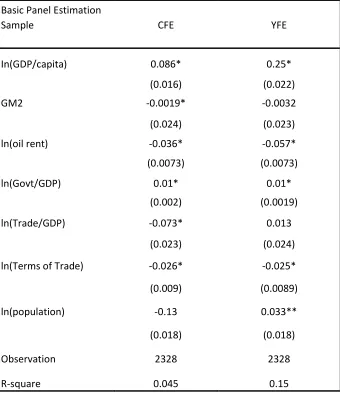
Table 4.1 presents the first set of results from the OLS estimation with
country fixed effect and year fixed effect. The dependent variable in this
regression is a dummy variable where 1 indicates a country is pegged and a 0
indicates it is not pegged. The standard errors in this regression are clustered at
the country level to control for serial correlation and for heteroskedasticity with
Column 1 which is estimated by linear probability (OLS) with country
fixed effect shows the basic panel results. Terms-of-trade is significantly
different from zero and its coefficient is negatively associated with fixed
exchange rate regime, indicating that countries attempt to switch to floating
exchange rate regime when they face negative terms-of-trade shock across time.
A negative terms-of-trade means the relative price of exports over imports
declines: one unit of exports will buy fewer imports. The purchasing power is
shrinking when terms-of-trade decreases. Countries likely to trade more with
the base are significantly more likely to peg, and those that are less likely to
trade with the base are less likely to peg. As expected, rich countries are less
likely to peg and those countries that with high oil rent more likely to peg.
Column 2 shows a set of result with country fixed effect and year fixed
effect. The purpose of adding year dummies is to capture global shocks that are
common to every country. Variables like GDP per capita, oil rent, government
spending and terms-of-trade are still consistent with column 1 and significantly
different from zero. Variables like trade has completely flipped sign between
country fixed effect and year fixed effect, implying that the specification in the
As it is stated earlier, one of the shortcomings of using linear probability
here is that it violates the assumption of OLS so that the estimators may be
biased. But we will see logistic model as a more accurate way in Table 4.2.
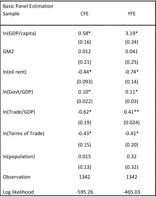
Table 4.2 presents the results by using logistic model which takes care of fixed
effect and heterogeneity. As similar as Table 4.1, column 1 shows the regular
logistic regression with counties fixed effect. Column 2 demonstrates the result
with adding year dummies. Now we see more clearly that coefficients on
terms-of-trade are negatively associated with fixed exchange rate regime choice and
significantly different from zero. Quantitatively, countries that face a negative
terms-of-trade shock are roughly 43% more likely to switch from peg to
floating regime. The economic rationale behind this is that if terms-of-trade is
unfavorable, the relative price of export over import becomes smaller. One unit
of exports will buy fewer imports in this case. The domestic purchasing power
is shrinking to some extent that countries with fixed exchange rate hit by these
shocks have fewer incentives to trade and intend to switch to floating exchange
rate to cushion the shock. In other way around, if countries face a positive
terms-of-trade shock, which the domestic purchasing power is on a rise and
exchange rate. This to a large extent explains the negative relationship between
terms-of-trade and the choice of exchange rate regime.
5. Concluding Remarks
The choice over fixed versus flexible debate remains highly contentious. In the
search for clearer answers, the theoretical arguments involved ought to be tested
and quantified. This paper presents the empirical analysis of how terms-of-trade
shocks affect the probability between choosing a fixed exchange rate regime
and floating one by using linear probability model and logistic model. It turns
out that the impact of terms-of-trade is negatively associated with fixed
exchange rate regime across countries and time period, as the literatures
indicate above. The impact of other variables on the choice of exchange regime
roughly follows the conventional studies of the matter.
In light of Milton Friedman’s hypothesis, in a world with sticky prices, the
nominal exchange rate could be used to insulate the economy against real
shocks. The reason why the nominal exchange rate may matter is the presence
after a negative real shock, output falls until wages and prices are (slowly) bid
down at a rate permitted by the nominal stickiness. In countries with a flexible
regime, by contrast, the monetary authority can respond to the shock by a
depreciation of the currency. The depreciation increases the domestic prices of
exported goods exactly when the international price of these goods has fallen
and thereby partially offsets the negative effect of the shock. Furthermore, the
currency depreciation reduces real wages at precisely the time when labor
demand has fallen, which also contributes to a smoother adjustment.
In the spirit of Friedman’s hypothesis, the more likely a country faces a real
terms-of-trade shock, the less likely it pegs its currency because a floating
exchange rate is able to smooth the shock in a faster way, without affecting
output too much if under a fixed exchange rate regime. Also from the data and
the graphs that shown in the section of literature review, we have seen
countries, especially developing countries flip the exchange rate regime from
fixed to floating, say, during 1997-1998, which witnessed the Asian financial crisis. My results confirm the prediction of Friedman’s theory because the time
span in the sample has witnessed no more than three recession period around
REFERENCES
[1] Baxter, M.,Stockman, A., 1989. Business Cycles and The Exchange Rate Regime. Journal of Monetary Economics.
[2] Broda, C., 2001a. Coping with Terms of Trade Shocks: Pegs vs.Floats.
American Economic Review.
[3] Broda, C., 2002. Terms of Trade and Exchange Rate Regimes in Developing Countries. American Economic Review.
[4] Ghosh, R., 2009. Toward a Stable System of Exchange Rate: Implications of Choice of Exchange Rate Regime.
[5] De Gregorio,J., Wolf, H., 1994. Terms of Trade, Productivity, and the Real Exchange Rate. NBER Working Paper 4807.
[6] Darne, O., Ripoll-Bersson,L., 2003. Exchange Rate Regime Classification and Real Performance: New Empirical Evidence.
[7] Juhn, G., and P. Mauro. 2002. Long-run Determinants of Exchange Rate Regimes: A Simple Sensitivity Analysis. IMF working paper.
[8] International Monetary Fund,1999. Exchange Rate Regimes in an Increasingly Integrated World Economy”.
[9] International Monetary Fund. Various dates. Annual Report on Exchange Arrangements and Exchange Restrictions.
[10] Juhn, G., and P. Mauro. 2002. Long-run Determinants of Exchange Rate
Regimes: A Simple Sensitivity Analysis. IMF working paper.
[11] Levy-Yeyati, E., Sturzenegger, F.,2002. To Float or to Fix: Evidence on
[12] Mundell, R. A. 1961. A Theory of Optimum Currency Areas. American Economic Review.
[13] Mundell, R. A. 1961. A Theory of Optimum Currency Areas. American
Economic Review.
[14] Shambaugh, J., Klein, M., 2007. The Dynamics of Exchange Rate
Regimes: Fixes, Floats, and Flips. Journal of International Economics
[15] Shambaugh, J.,2004 The Effects of Fixed Exchange Rate on Monetary
Policy
[16] Shambaugh,J., Obstfeld, M., Taylor, A.,2004. Monetary Sovereignty,
Exchange Rates and Capital Controls: The Trilemma in the Interwar Period. IMF Staff Papers.
[17] Savvides, A. 1990. Real Exchange Rate Variability and the Choice of
Exchange Rate Regime by developing countries. Journal of International Money and Finance.
[18] Shambaugh,J., and Klein, M., 2010. Empirics of Exchange Rate Regime
Choice. Exchange Rate Regimes in the Modern Era. The MIT Press.
Table 4.1. OLS Estimation
OLS estimation
Note: The dependent variable is peg status. Standard errors clustered at the country level below
coefficients. *significant at 5%. **significant at 10%. Sample is 91 countries from 1980-2007.
Basic Panel Estimation
Sample CFE YFE
In(GDP/capita) 0.086* 0.25*
(0.016) (0.022)
GM2 -0.0019* -0.0032
(0.024) (0.023)
ln(oil rent) -0.036* -0.057*
(0.0073) (0.0073)
ln(Govt/GDP) 0.01* 0.01*
(0.002) (0.0019)
ln(Trade/GDP) -0.073* 0.013
(0.023) (0.024)
ln(Terms of Trade) -0.026* -0.025*
(0.009) (0.0089)
ln(population) -0.13 0.033**
(0.018) (0.018)
Observation 2328 2328
Table 4.2. Logistic Estimation
Basic Panel Estimation
Sample CFE YFE
In(GDP/capita) 0.58* 3.19*
(0.16) (0.34)
GM2 0.012 0.041
(0.21) (0.25)
ln(oil rent) -0.44* -0.74*
(0.093) (0.14)
ln(Govt/GDP) 0.10* 0.11*
(0.022) (0.03)
ln(Trade/GDP) -0.62* 0.41**
(0.19) (0.024)
ln(Terms of Trade) -0.43* -0.41*
(0.15) (0.20)
ln(population) 0.015 0.32
(0.13) (0.32)
Observation 1342 1342
Log likelihood -595.26 -465.03
Logistic estimation
Note: The dependent variable is peg status; *significant at 5%. **significant at 10%. Sample period:
Appendix A: A list of countries used in the sample
Argentina Ghana Pakistan
Austrilia Greece Panama
Bangladesh Guatemala Paraguay
Beligum Honduras Peru
Bolivia
Hong Kong SAR,
China Philippines
Botsowana Hungary Poland
Brazil Iceland Portugal
Cameroon India Senegal
Canada Indonesia Seychelles
Cape Verde Ireland Singapore
Central African Rep. Israel Solomon Islands
Chile Italy South Africa
China Japan Spain
Colombia Jordan Sri Lanka
Congo,Dem.Rep. Kenya Sudan
Congo,Rep. Korea, Rep Swaziland
Costa Rica Lesotho Sweden
Cote d'lvoire Malaysia Swizerland
Denmark Mali Tanzania
Dominican Republic Malta Thailand
Ecuador Mauritius Tunisia
Egypt,Arab Rep. Mexico Turkey
Equatorial Guinea Morocco Uganda
Ethiopia Namibia United Kingdom
Fiji Netherlands United States
Finland New Zealand Uruguary
France Nicaragua Venezuela, RB
Gabon Niger Zambia