Performance Evaluation of Weighted Greedy Algorithm in Resource Management

University of Windsor University of Windsor

Scholarship at UWindsor

Scholarship at UWindsor

Electronic Theses and Dissertations Theses, Dissertations, and Major Papers

2018

Performance Evaluation of Weighted Greedy Algorithm in

Performance Evaluation of Weighted Greedy Algorithm in

Resource Management

Resource Management

Harjeet Singh

University of Windsor

Follow this and additional works at: https://scholar.uwindsor.ca/etd

Recommended Citation Recommended Citation

Singh, Harjeet, "Performance Evaluation of Weighted Greedy Algorithm in Resource Management" (2018). Electronic Theses and Dissertations. 7397.

https://scholar.uwindsor.ca/etd/7397

This online database contains the full-text of PhD dissertations and Masters’ theses of University of Windsor students from 1954 forward. These documents are made available for personal study and research purposes only, in accordance with the Canadian Copyright Act and the Creative Commons license—CC BY-NC-ND (Attribution, Non-Commercial, No Derivative Works). Under this license, works must always be attributed to the copyright holder (original author), cannot be used for any commercial purposes, and may not be altered. Any other use would require the permission of the copyright holder. Students may inquire about withdrawing their dissertation and/or thesis from this database. For additional inquiries, please contact the repository administrator via email

Performance Evaluation of Weighted Greedy

Algorithm in Resource Management

By

Harjeet Singh

A Thesis

Submitted to the Faculty of Graduate Studies through the School of Computer Science in Partial Fulfillment of the Requirements for

the Degree of Master of Science at at the University of Windsor

Windsor, Ontario, Canada

2018

Performance Evaluation of Weighted Greedy

Algorithm in Resource Management

by

Harjeet Singh

APPROVED BY:

H. Wu

Department of Electrical and Computer Engineering

J. Lu

School of Computer Science

J. Chen, Advisor School of Computer Science

DECLARATION OF ORIGINALITY

I hereby certify that I am the sole author of this thesis and that no part of

this thesis has been published or submitted for publication.

I certify that, to the best of my knowledge, my thesis does not infringe

upon anyone’s copyright nor violate any proprietary rights and that any ideas,

techniques, quotations, or any other material from the work of other people

included in my thesis, published or otherwise, are fully acknowledged in

accordance with the standard referencing practices. Furthermore, to the extent that

I have included copyrighted material that surpasses the bounds of fair dealing

within the meaning of the Canada Copyright Act, I certify that I have obtained a

written permission from the copyright owner(s) to include such material(s) in my

thesis and have included copies of such copyright clearances to my appendix.

I declare that this is a true copy of my thesis, including any final revisions,

as approved by my thesis committee and the Graduate Studies office and that this

thesis has not been submitted for a higher degree to any other University or

ABSTRACT

Set covering is a well-studied classical problem with many applications across

different fields. More recent work on this problem has taken into account the

parallel computing architecture, the datasets at scale, the properties of the datasets,

etc. Within the context of web crawling where the data follow the lognormal

distribution, a weighted greedy algorithm has been proposed in the literature and

demonstrated to outperform the traditional one. In the present work, we evaluate

the performance of the weighted greedy algorithm using an open-source dataset in

the context of resource management. The data are sampled from a given roadmap

with 1.9 millions of nodes. Our research includes three different cost definitions

i.e. location cost, driving cost and infrastructure cost. We also consider the

different coverage radius to model possible parameters in the application. Our

experiment results show that weighted greedy algorithm outperforms the greedy

DEDICATION

Dedicated to my parents Jaswant Singh and Paramjeet Kaur

ACKNOWLEDGEMENTS

I would like first like to thank my thesis advisor Dr. Jessica Chen for her valuable

guidance and continuous support during my research. She always steered me in the

right direction, and this work would not have been accomplished without her help.

I would also like to thank my thesis committee members Dr. Huapeng Wu and Dr.

Jianguo Lu for their valuable comments and professional assistance.

I would also like to thank Karen Bourdeau and the entire faculty of School

of Computer Science for their continuous support throughout the program. I would

like to express my profound gratitude to my parents and family members who were

the motivation and strength behind this work. Finally, I want to thank every one of

my friends who remained by amid great and awful circumstances.

TABLE OF CONTENTS

DECLARATION OF ORIGINALITY ... iii

ABSTRACT ... iv

DEDICATION ... v

ACKNOWLEDGEMENTS ... vi

LIST OF TABLES ... x

LIST OF FIGURES ...xi

LIST OF ABBREVIATIONS/SYMBOLS ... xii

CHAPTER 1 INTRODUCTION ... 1

1.1 Overview ... 1

1.1.1 Set Covering Problem and Its Applications ... 1

1.2Motivation ... 2

1.3Problem Statement ... 4

1.4Thesis Organization... 4

CHAPTER 2 REVIEW ... 5

2.1Dataset ... 5

2.2Matrix ... 6

2.3Coefficient of Variation ... 7

2.4Sampling... 7

2.5Set Covering Algorithms ... 10

2.6Literature Review ... 13

2.6.1 Deep Web Crawling Using a New Set Covering Algorithm ... 13

2.6.1.1 Hidden Web or Deep Web ... 13

2.6.1.2 Deep Web Crawling ... 14

2.6.1.3 Query Selection ... 14

2.7Set Cover Algorithms for Very Large Datasets ... 18

2.8Set Covering in Locating Facilities ... 22

CHAPTER 3 PROPOSED APPROACH AND EXPERIMENTAL SETUP ... 25

3.1Introduction ... 25

3.2Greedy Algorithm ... 25

3.3Weighted Greedy Algorithm ... 28

3.4Roadmap... 30

3.5Setup Procedure... 30

3.5.1Raw Dataset ... 31

3.5.2Connected Subgraph ... 32

3.5.3Coverage Graph ... 33

3.5.4Calculation of Coefficient of Variance ... 34

3.5.5Comparison of Greedy and weighted Greedy Algorithm ... 35

3.6An Illustrative Example ... 36

3.7.2 iGraph Library ... 42

3.7.3 R Studio ... 42

CHAPTER 4 EXPERIMENTATION AND RESULTS ... 43

4.1Data ... 43

4.2Cost Definition ... 46

4.3Results ... 47

4. 4 Impact of data distribution ... 49

CHAPTER 5 CONCLUSION & FUTURE WORK ... 54

5.1Conclusion ... 54

5.2Future Work ... 55

REFERENCES/BIBLIOGRAPHY ... 56

LIST OF TABLES

Table 2.1 The Input Matrix for Set Covering Matrix 15

Table 2.2 The initial table with weights based on Table 1 16

Table 2.3 Second round weighted matrix 17

Table 2.4 Results for the weighted greedy method 17

Table 3.1 Sample matrix of road network for greedy algorithm 27

Table 3.2 Sample matrix of road network for weighted greedy algorithm 29

Table 3.3 A 10-node connected subgraph 36

Table 3.4 01 Matrix of the Subgrap 37

Table 3.5 Matrix after division of node weights and calculation of nf, nw,

nf/nw

38

Table 3.6 Matrix after selection of the first node 38

Table 3.7 Matrix after second round 39

Table 3.8 Matrix after the third round 39

Table 3.9 Solution table for Weighted Greedy algorithm 39

Table 3.10 Matrix at the starting point for greedy algorithm 40

Table 3.11 Matrix after first round of greedy 40

Table 3.12 Solution table for greedy algorithm 41

Table 4.1 The properties of over data source under two types of data one 45

Table 4.2

with coverage radius 1 and other with variable coverage radius

Performance Improvement of Weighted greedy over greedy 47

algorithm regarding solution nodes in three different cost

definition scenarios

LIST OF FIGURES

Figure 2.1 A dataset representing connected nodes of a roadmap 5

Figure 2.2 Example of a Matrix 6

Figure 2.3 A Network Graph 6

Figure 2.4 An adjacency matrix for the above network graph 6

Figure 2.5 Sample input data 20

Figure 2.6 Inverted Index of Fig 1 20

Figure 2.7 Execution of algorithm by Graham. Et al. on sample data in fig 1 21

Figure 3.1 A Sample Graph 25

Figure 3.2 Flow of the approach 31

Figure 3.3 A 10-node connected subgraph 32

Figure 3.4 Coverage Matrix with coverage value 1 33

Figure 3.5 Connected Subgraph plot view 37

Figure 4.1 Distribution of node coverage degree in Coverage Radius 7 44

Figure 4.2 Distribution of node coverage degree in Coverage Radius 10 44

Figure 4.3 Distribution of node coverage degree in Coverage Radius 15 45

Figure 4.4 Cost difference of solution nodes under Driving Cost 48

Figure 4.5 Cost difference of solution nodes under Infrastructure Cost 48

Figure 4.6 Cost difference of solution nodes under Location Cost 49

Figure 4.7 Relationship between CV and improvement on Infrastructure

Cost regional maps

51

Figure 4.8 Relationship between CV and improvement on Location Cost 51

regional maps

Figure 4.9 Relationship between CV and improvement on Driving Cost 52

LIST OF ABBREVIATIONS/SYMBOLS

SNAP- Stanford Network Analysis Project

CV- Coefficient of Variation

P2P- Peer to Peer

RE- Random Edge

RNE- Random Node-Edge

SCP- Set Covering Problem

DF- Document Frequency

QW- Query Weight

MCLP- Maximal Set Covering Problem

NCD- Node Coverage Degree

NNF- New Nodes Fetched

NW- Node Weight

CHAPTER 1

INTRODUCTION

1.1

Overview

One of the most common problems today is the planning. Planning includes making

plans about where to build new facilities in a city, how to allocate the resources and how

to use the resources optimally. Solutions to these problems exist with many techniques,

and one of them being the solution to the set covering problem. Finding the smallest set

of solutions of a problem from many sets of solutions is widely researched in many

fields. A set covering problem is presented as an abstract problem, so it captures many

different scenarios in the context of knowledge mining, data management, etc. [1].

1.1.1 Set Covering Problem and Its Applications

Set covering is a classical problem in the field of computer science. It is one of the

Karp’s 21 NP-complete problems. This problem is a base for the entire field of

approximation algorithms. Set covering is considered NP-Hard in optimization and

search problems and NP-Complete in decision-based problems.

Set Covering is to select a minimum number of subsets in such a way that they

contain all the elements from a fixed universe [2]. The most significant factor considered

in this process is to minimize the cost of the selected subsets. There are various

applications of set covering. Some of them are as follows [1].

Operational Research: - The operational research problem is to locate a facility in such

a way that specific sites can reach it. This problem can be solved using set covering

Machine Learning: - In machine learning, items are classified based on examples that

cover them. The final goal is to make sure that all items are covered by some example,

which is an instance of Set Covering problem.

Planning: - In planning, set covering can be applied to allocate resources when demands

vary over time. To cover the requirements for planning, variations of set covering are

used [3].

Data Mining: - Set covering can be applied to find the minimal explanations for the

patterns in the data. In data mining, the goal is to find a set of features in such a way that

every example is a positive example of these features. It can be viewed an instance of set

cover problem where each set contains some examples which correspond to a feature.

Information Retrieval: - In Information Retrieval, the goal is to find the smallest set of

documents that cover the topics in a query. It leads to an instance of set cover where a set

of documents is required in response to a query[4].

1.2

Motivation

In this world, if we want to complete any task we need some resources. Everything and

everyone need resources to complete its functioning whether a human being or a

machine. Management of these resources is a problem which needs to be studied to get

the best use of these resources that we have and to use them for a more extended period.

When we think of resource management in the field of planning, there are various

problems which need to be addressed.

In strategic planning for big firms whether private or public, facility location is a

Operational Research is a well-established area in itself [32]. There are various models in

this area to help with the decision-making process, and one of the most popular areas in

those models is facility location model in covering problem. The concept of covering

comes from its applications in daily life. Some of the problems are to determine the

number and the location of public facilities like schools, libraries, hospitals, parks, fire

stations and various other places.

Another major factor of studying in this area is the need to plan things properly. The

rapid growth of population concerning some available resources has forced us to think of

solutions to provide resources to people in such a way that demand can be managed in the

best possible way. One daily life application of this is the placement of fire stations in a

city in such a way that those fire stations can cover the entire area of the city and that the

number of those stations is minimized to reduce the operational cost and initial

investment in the infrastructure.

Another part that motivated this thesis work is set covering problem. It is a part of Karp’s

Np-complete problems, a base of approximation algorithms, that had led to the

development of various fundamental techniques in this field. The usefulness of set cover

problem has been seen at many places of the exciting application.

The weighted greedy algorithm by Wang et al. [16] is a good variation of greedy

approach for web crawling but hasn’t been tested on any other type of set covering

problem. The use of this solution within the field of resource management might give

1.3

Problem Statement

As the world is dealing with the shortage of resource, there arises a need to either get

more resources or to manage those resources appropriately. Study on set covering has

provided many useful results for planning and resource management problems.

A weighted greedy algorithm for set covering problem has been proposed by Wang

et.al.[16] within the context of web crawling and demonstrated to outperform the

traditional greedy algorithm. In our present work, we evaluate the performance of the

weighted greedy algorithm using open-source datasets in the context of resource

management. It includes the setting of resource allocation on a sample taken from a

roadmap with 1.9 million of nodes. The dataset is taken from open source data provided

by Stanford Network Analysis Project (SNAP)[35].

1.4

Thesis Organization

The rest of this thesis is organized as follows: Chapter 2 provides a review of some of the

concepts and terminologies that are related to this work and provides more details of the

areas related to this research. It also includes a review of some of the closely related work

of other researchers. In Chapter 3, we define the problem and present the proposed

approach. Chapter 4 shows the results of experiments and Chapter 5 concludes the thesis

CHAPTER 2

REVIEW

2.1

Dataset

A dataset is a collection of data most commonly corresponding to a database table or

matrix where rows and columns define some values. They are large in size and might not

be well organized like a database. Most of the times a data set is a collection of data

under some experiment. For example:- Temperature data gathered by a probe for every

half an hour for one month.

Fig 2.1: A dataset representing connected nodes of a roadmap

In the above, the dataset for connection among nodes is represented. There are various

ways to represent a dataset. It can be a numeric matrix, adjacency matrix or a table with

2.2

Matrix

A two-dimensional array of numbers arranged in rows and columns is called a matrix.

The size of a matrix is determined by its number of rows and columns. Usually, rows are

listed first and the columns second. Let’s say if a matrix is said to be 3 * 4 then it has

three rows and four columns.

Fig 2.2: Example of a Matrix

Various operations can be performed on a matrix like Addition, Scalar Multiplication,

and Transposition, etc. There are various types of matrix used in various applications. For

example, in Graph Theory, the transpose matrix is used to represent the connection

among nodes.

Fig 2.3: A Network Graph

1 1 0 1 0 1 0 1 0

2.3

Coefficient of Variation

The coefficient of variation (CV) is a measure of relative variability. It is the ratio of the

standard deviation to the mean and is also known as a relative standard deviation. Its

most common use is in the field of engineering and physics for quality assurance studies.

The biggest advantage of the coefficient of variance is that it is unitless. It is used to

represent the consistency of the data. Here consistency means the uniformity of data

distribution. We can also use it to compare two datasets or samples. The coefficient of

variation is also denoted by CV:

�

(2.1)

Here S stands for standard deviation and X stands for a mean of the sample. The use of

CV is limited to some conditions. For example, it should be computed only for data

measured on a ratio scale and only for non-negative values. It cannot be used for data on

an interval scale.

There are some disadvantages when we use CV under certain conditions. For example

Coefficient of Variation will reach infinity, if the mean is close to zero and it is sensitive

to small change in the mean.

2.4

Sampling

The first thing comes to mind when one tries to perform some experiment on big data is

how to handle big data or how to perform tests on such a big size of data. The technique

most commonly used is sampling. A small subset of original data is taken out to perform

the tests, and it is assumed if the experiment is right in a sample then it should also

perform well on the original data.

Why reduce data?

i.It is not always possible to store all the data.

ii.It is too resource consuming to work with big data.

iii.It is faster to work with a smaller amount of data.

Why Sample?

There are several reasons why we use sampling approach rather than applying direct

experimentation on original data. Some of the reasons are:

i.Estimation on a sample is easier and more straightforward.

ii.It is easy to understand.

iii.Sampling is general and is independent of the analysis to be done.

How to take a sample of original data?

Now the question arises how to take a sample. For that, there are various sampling

algorithms available. Some mostly used are as follow:

Random Walk:- First we pick a random node and then start a random walk on the graph

[5]. The next node is selected with a certain probability, the probability by which vertices

and edges are sampled [6]. If the random walk is struck at some point, it gets back to a

Sampling by random node selection:- In random node selection, starting node is

selected randomly, and then the next node is selected based on the probability of the node

being selected. This probability could be either proportional to the page rank weight [5]

of the node, or proportional to a degree of a node, i.e., with how many nodes it is

connected. It can be used in peer to peer (P2P) networks like Bit torrent [6].

Sampling by random edge selection:- This is similar to node selection, while edges are

randomly selected. It is known as Random Edge (RE) Sampling. The only difference in

this one compared to random node selection is that we select edge rather than nodes. A

variation of this model is Random Node-Edge (RNE) sampling, in which, first at random,

a node is selected and then uniformly at random, an edge corresponding to the node is

selected [5].

Forest Fire Model [8]:- In this model, we pick a random seed node and then begin

burning outgoing links and corresponding nodes. Once a node is burned, the node at the

other end has a chance to burn its link which will continue recursively. For example, a

new graduate student arrives at a university and gets acquaintance with some senior

students from his department. Those students introduce him to their friends, and those

friends may introduce him to their friends which make it a recursive process. This

process needs two parameters: a forward burning probability, and a backward burning

ratio.

Snowball Sampling Approach [7]:- A snowball sampling approach is something similar

and it can also be carried out without the probability, using a deterministic approach. As

the name suggests, it starts with a random node and then grows like a snowball by

collecting all the corresponding nodes to that random node and continues.

2.5

Set Covering Algorithms

For set covering algorithms, we first need to know what set covering problem is and what

the desired solutions are.

The Set Covering Problem is where we have a given set of elements (A finite universe)

M = {e1, e2, . . . , em} and a set of subsets of M, X = {S1, S2, . . . , Sn}. Each subset has

a non-negative cost Ci. We have to find a union of subsets U{Si} which has minimum

Cost (C) and contains all the elements of M.

The formal definition of set covering is:

I ⊆ {S1, S2, . . . , Sn} that minimizes ∑ (i∈I)Ci and guarantees ⋃(i∈I)Si=M

Set covering problem is also defined on the 0-1 matrix by Carpara and Toth [9]:

Let A=(aij) be a 0-1 m x n matrix, and c= (cj) be an n-dimensional integer vector. The

value cj (j ∈ N) represents the cost of column j, assuming that cj > 0 for j ∈ N. j ∈ N

covers a row i ∈ M if aij=1. SCP calls for a minimum-cost subset S of columns, such that

each row i ∈ M is covered by at least one column j ∈ S. A natural mathematical model

for SCP is

v(SCP)= min∑∈N CjXj (2.2)

∑∈N AijXj ≥ 1 , for all i ∈ M, (2.3)

xj∈ {0,1}, j ∈ N (2.4)

Here Equation (2) makes sure that each row is covered by at least one column and

Equation (3) is the integrality constraint [2].

The set covering problem is an NP-Hard problem, and there are many algorithms

to solve it. There are two ways to solve this problem: exact algorithms and heuristic

algorithms. The exact algorithms are mostly based on branch and bound and branch and

cut [12]. The Best exact algorithm for the SCP is CPLEX [14]. Greedy algorithms may

be the best fit to solve the significant combinatorial problems quickly. A greedy

algorithm is discussed in more detail below.

2.5.1 Greedy Algorithms for Set Covering Problem

Greedy algorithms are a type of heuristic algorithms. There are various reasons why they

are used so much. According to [11,15], greedy set cover algorithms are best known

polynomial-time approximation algorithms for set cover. They are easy to implement,

and that is why they are most commonly used heuristic algorithms.

Classical Greedy Algorithm:- This is the most basic greedy algorithm. It selects the set at

each step which contains the largest number of uncovered elements. The process

continues until all the elements are covered. Let (X, F) be an instance of set covering

is the solution which is initially empty, and S is a single subset. Then the Greedy

Algorithm will work like this:

Greedy Set Cover (X, F)

1 U <- X

2 C <- Ø

3 While U≠ 0 do

A.

Select an S

∈

F that maximizes |S ∩ U|

B.

U <- U - S

C. C <- C U {S}

4 return C

Example: Let X = { a, b, c, d, e, f, g, h, i, j} be a universe and F = {{a, b, c, d, e, f}, {a, b,

c, g, h}, {d, e, f, i, j}, {g, h, i}, {j}} and let labels for these subsets be S1,S2,S3,S4,S5

respectively. Initially, C is empty. In the first step, the greedy algorithm will select S1 =

{a, b, c, d, e, f} because coverage of this subset is better than all other subsets. Now

solution set is C = {{a, b, c, d, e, f}}.

In the second step, S4 has the most substantial number of uncovered elements {g, h, i},

i.e., the greedy algorithm will choose S4 and now solution set C = {{a, b, c, d, e, f}, {g,

h, i}}.

In the third step, S2 has one uncovered element {j} and S5 has one uncovered element

{j}. Either one of them can be selected. Let us selected S5, so now the solution set will

the final solution set. The greedy algorithm might not give optimal solution every time,

but the result is most of the time good enough. Considering the simple implementation, it

is worth using it.

There are many variations of Greedy algorithms people use according to their needs, for

example, weighted greedy algorithm. In this type of greedy algorithm, weight is assigned

to every node which tells the importance of the node, and by how many nodes it is

covered. In this situation, we can select a different strategy. For example, if a single node

is covered by many nodes then we can say that this node can be added to result later and

we try to get the least covered node into the result first. There are many other ways to

modify greedy algorithm according to the needs.

2.6

Literature Review

2.6.1

Deep Web Crawling Using a New Set Covering Algorithm

In this paper [16], the authors described a new set covering algorithm for crawling in the

deep web. To understand the concepts of this paper, first, we need to know hidden web,

web crawling, and query selection. We give a brief explanation of these.

2.6.1.1

Hidden Web or Deep Web

A deep web is referred to as a web-generated from the file system and database and

cannot be accessed by URL directly. It is often guarded by search interfaces. Most of the

people depend on search engines like Yahoo, Google, etc. to find information on the web

but these web search engines only search the surface web. It is estimated that deep web is

nearly 550 billion documents which are up to 2,000 times greater than surface web.

Hidden Web has more focused content than Surface Web entities.

2.6.1.2

Deep Web Crawling

Fetching the information from the hidden web is termed as deep web crawling. A query is

issued which contains some keywords, and with those keywords in the query, we crawl

the data from the hidden web. For crawling the deep web, crawlers are used which is a

GUI based interface between the web and the user. Hidden Web Crawlers search the

hidden website using the given query, and then they give back the results based on the

query.

2.6.1.3

Query Selection

It is the process of selecting queries that can cover a maximum number of documents in a

corpus. It is an essential step because if the format of a query is not proper, it may give an

empty result [18]. According to [17], one should also consider the cost of the query

because sometimes some queries might give good results but at the stake of a significant

query cost which is not acceptable.

Now that we know some basics about web crawling let's get back to the paper by Wang

et al. [16]. In this paper, the authors used set covering with greedy and weighted greedy

algorithm for the deep web crawling. The primary task is to select a proper set of queries

to minimize the total cost of mapping selected queries into the original database.

They created a four-step framework for deep web crawling:

ii.Create a query pool, i.e., a set of queries based on sampleDB.

iii.By using sampleDB and query pool, select a proper set of queries.

iv.Map those selected queries to the original database.

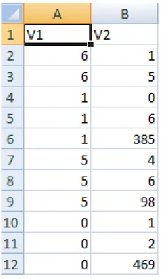
For example, Table 2.1 shows an input matrix for the set covering algorithm. Here {d1,

d2, ..., d9} represents documents of a sample database. {q1, q2, ...., q5} represent

queries. Let this table be a sample from the original database. Suppose that we run the

algorithm on a sample rather than directly on the corpus. Queries selected from a sample

database can also perform on the original data source as well [21].

Table 2.1: The Input Matrix for Set Covering Matrix

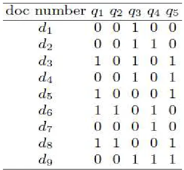
According to a simple greedy algorithm for unit cost, next query q is the one

which covers the maximum number of new documents. Here the authors are using a

weighted greedy algorithm. Therefore, they add weights to the documents. It will help to

cover small documents first because they can be matched with few queries. Smaller

According to greedy strategy, queries QJ with larger query weight (qw) are preferred. A

large qw should be obtained by a small number of documents. In other words, queries

with smaller df/qw are preferred. Therefore weighted greedy algorithm will choose next

query with smaller df/qw.

For example Table 2 shows the weights based on Table 1. At the bottom of the

table, document frequencies and query weights are listed. Here the smallest value for

df/qw is 1.85 for q4. q4 is selected, and documents covered by that query are removed

from the matrix. See Table 3 for the matrix in the second round.

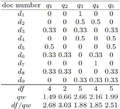
Table 2.3: Second round weighted matrix

See Table 2.3 now, it has only four queries and five documents left. The process

continues until all the documents are removed from the matrix. Table 4 shows the final

results of the weighted greedy method. Here q4, q3, q1 are selected in the first, second

and third round respectively.

Table 2.4: Results of the weighted greedy method.

Here the cost is how many total documents can a query fetch. The unique rows column is

how many total unique documents are fetched by queries after a certain point. For

cost after selecting q4 and q3 is 9. q3 can fetch three new documents which means three

unique rows. The unique rows fetched by q4 and q3 are 7.

The above picture shows the weighted greedy algorithm in [16]. This method performs

better than the greedy algorithm as the experiment shows.

Therefore we will be using this same approach in operational research and provide the

comparison to see if this weighted greedy method performs better in other scenarios.

2.7

Set Cover Algorithms for Very Large Datasets

Graham et al. [1] showed how to work with large datasets to find a solution to the set

covering problem with a standard greedy algorithm. They gave an alternative approach to

the greedy algorithm, particularly for disk-resident datasets. The most backdated research

on this topic is by Berger et al. [11]. The idea of Berger is recently applied to Map

They considered a standard unweighted greedy algorithm for the set covering problem.

The most significant problem for a greedy algorithm is the use of memory because, for

every update of the set, it needs to access information from a disk or access the main

memory. Although modern computers have a significant amount of memory, efficient use

of memory is necessary. For example, random access to disk will be highly expensive.

Graham et al. [1] analyzed the algorithms for external memory model of the running

during the execution.

They presented a greedy heuristic using two approaches, inverted index, and multiple

passes.

Inverted Index:- This approach is suitable when random access to a location in the

memory takes a constant amount of time. In inverted index approach, a priority queue is

maintained for each Si\C. The priority queue is a descending order queue of set Si. Here

Si denotes the collection of m subsets of the universe and C denotes elements covered so

far. To update values of Si\C, when a set Si is added to the solution, it is needed to

determine which other sets contain elements of Si. This step can be done using inverted

index in which each item j is associated with

Tj={i:j S

}

(2.5)

Tj is the inverted index of Si. Tj is created in preprocessing step, and greedy iteration is

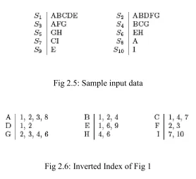
Fig 2.5: Sample input data

Fig 2.6: Inverted Index of Fig 1

This algorithm is expensive due to many random accesses to many locations on disk. It is

also tough to predict at which stage Tj will be used.

Multiple Passes:- This approach does not use any priority queue or inverted index. It

merely keeps track of set C covered so far. In this approach, every time two sets are

compared, we look for those already covered elements in those not selected sets. It

makes linear passes through the data which is efficient when the data is resident on the

disk. The only disadvantage is that it will be slow if the size of a selected set is large

because it might need to go through the entire dataset to add this set.

Graham et al. give a new approach which is better than the standard greedy algorithm.

Their approach follows the subsetting of sets according to the size of the sets. Their

algorithm works in two loops. They added a parameter p>1 to govern the approximation

The algorithm by Graham et. al.

Initially, Si is assigned to sub-collection S(k) if pk Si<pk+1.Here in the algorithm, K is

the largest k with nonempty S(k). Figure 3 shows the algorithm execution on sample

input data in Figure 2.7.

Fig 2.7: Execution of algorithm by Graham. Et al. on sample data in fig 1

The basic functionality of this algorithm is to arrange the sets according to their sizes.

range are reduced to only uncovered elements and appended to the corresponding range

of sets. This process continues until all the elements in the universe are covered. The

proposed algorithm according to the results is much faster than the conventional

algorithms.

This paper gave us an idea to use greedy and variation of greedy with large datasets. We

are interested in seeing the behavior of this algorithm in operational research when data is

large. The approach followed by this paper was to test on disk-resident data and memory

resident data. We are using the leanings from memory resident approach to do our

experiments.

2.8

Set Covering in Locating Facilities

In the planning strategy of big public and private firms, facility location is a critical

component of the study. In facility locating, covering models are most extensively

studied. They are such attractive topics for researchers because of their applicability in

the real world. In covering models, the customer can get service from a facility in a

predefined area. That predefined distance is called coverage distance or coverage radius

[23]. According to Schilling et al. [24], Set covering models can be classified into two

major categories: Set Covering Problem (SCP) and Maximal Covering Location Problem

(MCLP). The difference between these two is that in SCP, the coverage is required and in

MCLP, the coverage is optimized. Classification can also be given based on the solution,

i.e., heuristic or optimal.

According to Reza et. al.[25], the first covering model was introduced by Hakimi in 1965

police needed to cover all the nodes on a highway network. The first mathematical

problem was developed by Toregas et al. [27]. It was used for the location of emergency

service facilities. We are going to discuss various set covering approaches for locating

facilities.

Another paper by Toregas, Swain, et al. [30] gives an emergency vehicle model with a

specified time or distance constraint which is on demand. If this kind of constraints is

given, then the problem is either to find a solution with minimum time or distance or to

find a solution with a minimum number of facilities. They have assumed that the time

needed between every two user nodes is known, and the upper limit for the constraint like

time or distance can be described. If maximum response time for a node is s, then for any

node I that is at most s time away from I, we can provide the emergency service to i. Ni

denotes this set for node i. They give a mathematical problem as follows

xj ={ 0 if no facility is established at point j,

xj={1 if a facility is established at point j.

The actual implementation of (I) requires two steps. In the first step, it determines the sets

Ni for a given value of s and a given shortest distance matrix. The second step involves

A paper by Mark S. Daskin [28] describes the stochastic approach for set covering. They

used a heuristic algorithm to solve the problem. They considered the problem of covering

a location with more than one facility so that in case one facility is not operating; the

other can be reached. They have given an algorithm which describes in the case of

CHAPTER 3

PROPOSED APPROACH AND EXPERIMENTAL SETUP

3.1

Introduction

This chapter introduces the use the weighted greedy algorithm proposed by Wang. Et.

al.[16] in the field of resource management. As demonstrated in the paper, it has

outperformed the traditional greedy algorithm in the field of web crawling for query

selection. Our objective here is to compare the performance of the weighted greedy

algorithm with the traditional greedy algorithm in roadmaps.

3.2

Greedy Algorithm

Greedy algorithms are a type of heuristic algorithms. A greedy algorithm always looks

for a locally optimal solution. Greedy might not find a globally optimal solution, but it

will provide an answer very close to the optimal one with less processing cost. Greedy

Algorithms are used in various fields like networking, machine learning, artificial

intelligence, etc.

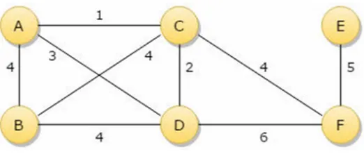
Fig 3.1: A Sample Graph

Figure 3.1 is a sample graph. Suppose that we want to apply a greedy algorithm on this

shortest path is C to F, F to E and the total cost is 9. According to the Greedy algorithm,

it will choose the shortest path at a particular instance. Therefore, the path will be C to A,

A to D, D to F, F to E and the total cost will be 15. The path chosen by greedy algorithm

is not optimal all the time. It only looks for best option at a particular instance. It can be

used in multiple scenarios and setups. There are several algorithms used in the set

covering based on a greedy approach to solve the problems.

The basic greedy algorithm uses the step by step approach to solve the problem, and at

every step, a solution node is chosen for this problem. Greedy is to approximate the

globally optimal solution using the locally optimal solution on each step. For every step,

one column is selected, and there are various ways to select a column. A column here

represents a node.

There are various approaches to apply the greedy approach, it all depends on which factor

we want to focus on. Some of the approaches on which solution can be focused are as

follows:

• Minimize the cost: The next column is selected which has the lowest cost on a

particular step. Using the smallest cost at every step, lowest total cost is

approximated.

• Maximize coverage: Another method is to select the next column which can

cover the largest number of nodes that are not yet covered by previously selected

• Combined Approach: We can also use the combined approach which combines

both the above approaches and take into consideration cost and the number of

new nodes that can be covered.

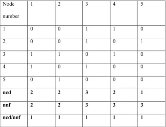
Node

number

1 2 3 4 5

1 0 0 1 1 0

2 0 0 1 0 1

3 1 1 0 1 0

4 1 0 1 0 0

5 0 1 0 0 0

ncd 2 2 3 2 1

nnf 2 2 3 3 3

ncd/nnf 1 1 1 1 1

Table 3.1: Sample matrix of road network for greedy algorithm

The above matrix represents the input matrix to the greedy algorithm. Here ncd is node

coverage degree which means how many nodes can be covered by a node. nnf is new

nodes fetched, i.e., how many new nodes can be fetched by this node. Initially, nnf is the

same as node frequency, and it changes after some iterations. ncd/nnf is to determine

3.3

Weighted Greedy Algorithm

In weighted greedy algorithms, the approach is the same to choose the best at a particular

instance. The only difference is that there are weights added to the nodes which have a

crucial role in deciding for a particular instance to determine which one is the best. The

weighted greedy algorithm, which is used in our approach, is based on choosing the

nodes which are less covered, which means areas that are less accessible are covered first.

The algorithm is as follows:

Node

number

1 2 3 4 5

1 0 0 0.5 0.5 0

2 0 0 0.5 0 0.5

3 0.33 0.33 0 0.33 0

4 0.5 0 0.5 0 0

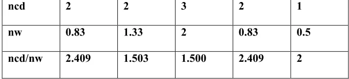
ncd 2 2 3 2 1

nw 0.83 1.33 2 0.83 0.5

ncd/nw 2.409 1.503 1.500 2.409 2

Table 3.2: Sample matrix of road network for weighted greedy algorithm

Here ncd stands for node coverage degree, nw for node weight which is the sum of the

significance of all nodes and ncd/nw is used to pick the next solution node. Here node

significance stands for the out degree of a node, i.e. the total sum the column of this node

in the matrix.

According to the algorithm, more focus should be put on nodes with less coverage, i.e.,

nodes that can be reached by less number of nodes. As for greedy strategy, nodes with a

large number of node weight are preferred, i.e., small nf/nw is preferred.

In the greedy algorithm, it does not matter whether a node is covered later or early, but

this is important in the weighted greedy method. In the above table, node 5 is only

covered by node 2, so it is essential to cover this node first. We argue that for each node i,

if the number of the nodes covering node i is bigger, it is better covering node i later. The

reason for this is:

When node i is covered in later steps, more columns covering node i means that there is a

When node i is covered in earlier steps, there is a higher possibility of overlapped

coverage, because node i will be covered multiple times when more columns will be

covering this node.

3.4

Roadmap

Here term roadmap is coined as a network of roads for a particular area demonstrated in

the form of edges and vertices. Every node or vertex represents an intersection, and every

edge is a link between those nodes. These roadmaps can be created from the data

provided in the form of a matrix. Usually, the 0-1 matrix represents which node is

connected to the other node.

3.5

Setup Procedure

The primary purpose of our experiment is to test the performance of the weighted greedy

algorithm in resource management and compare it with the greedy algorithm regarding

solution results. We will run greedy and weighted greedy algorithm on datasets with 100

samples, 50 for coverage radius 1, and 50 for variable coverage radius, using three cost

definitions.

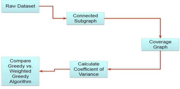
Fig 3.2: Flow of the approach

The raw dataset, Connected Subgraph, and Coverage Graph are the part of data

preprocessing where data is being converted into the suitable format as an input for

greedy and weighted greedy algorithm. Calculation of Coefficient of Variance is being

done as a parameter to compare both algorithms. The last module is a comparison of

Greedy vs. Weighted Greedy algorithm where both the algorithms are implemented and

executed on same input data to test their performance.

3.5.1

Raw Dataset

Raw Dataset is the original data obtained from the SNAP(Stanford Network Analysis

Project)[35]. We are using the dataset which is road network of California. Road network

for California contains 1,965,206 Nodes and 2,766,607 Edges. This raw dataset is in the

form of a matrix with two columns where column 1 denotes the node from which

3.5.2

Connected Subgraph

Working with big data is always a difficult task. There are several issues like memory

and hardware resources we have to deal with and to avoid these problems we are using

the connected subgraphs of smaller size from these raw datasets. The connected

subgraph, as the name suggests is a small portion of the original data coined as a sample.

We are using the sample size of 10,000 nodes approximately. This sample is a matrix

same as the raw dataset but with smaller size and with all the connection among those

selected nodes from the raw dataset.

Fig 3.3: A 10-node connected subgraph

The above figure 3.3 is an example of connected subgraph with 10 nodes fetched from a

raw dataset with all the connection among the nodes. We are using this kind of connected

3.5.3

Coverage Graph

It is the adjacency matrix generated from connected subgraph. The coverage graph is

generated according to the defined coverage. Here coverage is how many nodes can a

node cover starting from its neighbors. If we say the coverage graph has coverage value

of two, then we can say that a node can cover its neighbors and neighbors of their

neighbors. As the coverage value increases, more levels of neighbors each node will

cover. The coverage graph is represented in the form of adjacency matrix where 1

denotes that the node can cover that node and 0 denotes it cannot cover that node.

Fig 3.4: Coverage Matrix with coverage value 1

The above matrix is a representation of connected subgraph in the form of coverage

graph where each row represents which nodes a single node can cover. For example, in

second-row, node 9 can cover 7, 10 and 84. This matrix has coverage 1, i.e., a node can

cover its neighbors only. If this node has coverage 2 then the same node 9 could have

110, 83 and 85. This coverage graph acts as input for the greedy and weighted greedy

algorithm.

3.5.4

Calculation of Coefficient of Variance

This part calculates the coefficient of variance which is used as a parameter to compare

the performance of both the algorithms. The coefficient of Variance (CV) is calculated

using the standard formula which is standard deviation divided by the mean of the

sample. Once the CV is calculated, we can test the performance of algorithms and

analyze for a specific CV range how much improvement our algorithms show. For every

sample, we calculate the CV once.

In our case, we are calculating the CV of a sample using the formula used by Yan Wang

[34] in his approach. We measure the dispersion of node degree (deg) using Coefficient

of Variation. We know that the CV is the ratio of standard deviation to the mean, where

mean is the sum of the node degree over the total number of nodes in the sample.

(3.1)

Mean here can also be called an average node coverage degree. In the same way, we will

calculate the standard deviation of the sample which is

Here deg is the degree of a node and µ is the mean calculated above, and m is a total

number of nodes in the sample. By definition of this standard deviation and mean, we

calculate the value of coefficient of variation (CV) which is

(3.3)

Once the CV is calculated for the sample, we can compare the algorithms and calculate

the improvement of weighted greedy over the greedy algorithm.

3.5.5

Comparison of Greedy and weighted Greedy Algorithm

In this step, a coverage graph with specific CV is supplied as an input to both the

algorithms and the algorithms perform their calculations to compute the solution

outcome. The solution contains two different answers, one from greedy and one from

weighted greedy. The solution contains the number of solution nodes given by each

algorithm. Then those solutions are compared using the improvement formulae to check

how much improvement the weighted greedy algorithm has over greedy algorithm.

−

(3.4)

Formulae to check the improvement

The above formula calculates the improvement of the weighted greedy algorithm over

greedy algorithm. Here Cg and Cw are the results (total cost) for greedy and weighted

greedy respectively.

After calculating the improvement, the data is plotted on the graph which represents the

improvement correlated with CV.

3.6

An Illustrative Example

Here we will show an example of a small data to illustrate the working process. We will

start with a small dataset represented above with ten nodes and illustrate the process on

that dataset. Suppose that we have fetched the following subgraph from the raw dataset

Table 3.3: A 10-node connected subgraph

Fig 3.5: Connected Subgraph plot view

Now we convert this subgraph into an adjacency matrix with the coverage radius 1. The

matrix produced is as follows:

Table 3.4: 01 Matrix of the Subgrap

Now we consider applying the weighted greedy algorithm on this matrix and calculate

the node coverage degree(ncd), node weight(nw) and nf/nw. First, we add all the values

index. We will perform this step for every individual row, and the resulting matrix is as

follows

7 9 10 84 11 110 12 83 112 85 111

7 0 1 0 0 0 0 0 0 0 0 0

9 0.333 0 0.333 0.333 0 0 0 0 0 0 0

10 0 0.25 0 0.25 0.25 0.25 0 0 0 0 0

84 0 0.25 0.25 0 0 0 0 0.25 0 0.25 0

11 0 0 0.333 0 0 0.333 0.333 0 0 0 0

110 0 0 0.25 0 0.25 0 0 0 0.25 0 0.25

12 0 0 0 0 1 0 0 0 0 0 0

83 0 0 0 0 0 0 0 0 0 0 0

112 0 0 0 0 0 0.333 0 0.333 0 0 0.333

85 0 0 0 1 0 0 0 0 0 0 0

111 0 0 0 0 0 0.5 0 0 0.5 0 0

ncd 1 3 4 4 3 4 1 2 3 1 2

nw 0.33 1.5 1.116 2.083 1.5 1.416 0.333 0.583 1.25 0.25 0.583

ncd/nw 3.03 2 3.43 1.92 2 2.82 3.03 3.43 2.4 4 3.43

Table 3.5: Matrix after division of node weights and calculation of nf, nw, nf/nw

We select the value with smallest nf/nw. Now 84 will be added to the solution and

column with node 84 and all rows of nodes it covers will be deleted including 84. The

resulting matrix after this step will be

7 9 10 11 110 12 83 112 85 111

7 0 1 0 0 0 0 0 0 0 0

11 0 0 0.333 0 0.333 0.333 0 0 0 0 110 0 0 0.25 0.25 0 0 0 0.25 0 0.25

12 0 0 0 1 0 0 0 0 0 0

112 0 0 0 0 0.333 0 0.333 0 0 0.333

111 0 0 0 0 0.5 0 0 0.5 0 0

nc d 1 3 4 3 4 1 2 3 1 2

nw 0 1 0.583 1.25 1.166 0.333 0.333 0.75 0 0.583 ncd/n w Inf 3 6.861063 2.4 3.430532 3.003003 6.006006 4 Inf 3.430532

Table 3.6: Matrix after selection of the first node

Now we again select the minimum values for nf/nw, and node 11 will be selected. The

same process will be repeated, and column with node 11 and rows covered by this node

7 9 10 110 12 83 112 85 111

7 0 1 0 0 0 0 0 0 0

112 0 0 0 0.333 0 0.333 0 0 0.333

111 0 0 0 0.5 0 0 0.5 0 0

ncd 1 3 4 4 1 2 3 1 2

nw 0 1 0 0.833 0 0.333 0.5 0 0.333

ncd/nw Inf 3 Inf 4.801921Inf 6.006006 6 Inf 6.006006

Table 3.7: Matrix after second round

In the same way, after the third round now the selected node will be 9, and the same

process will be repeated. In the fourth round, selected result node will be 110, and all the

rows will be deleted.

7 10 110 12 83 112 85 111

112 0 0 0.333 0 0.333 0 0 0.333

111 0 0 0.5 0 0 0.5 0 0

nf 1 4 4 1 2 3 1 2

nw 0 0 0.833 0 0.333 0.5 0 0.333

nf/nw Inf Inf 4.801921 Inf 6.006006 6 Inf 6.006006

Table 3.8: Matrix after the third round

The nodes selected as result nodes are 84,11,9,110

node nf nw Nf/nw cost Unique rows

84 4 2.08 1.92 4 5

11 3 1.25 2.40 7 8

9 3 1 3 10 9

110 4 0.83 4.80 14 11

In this example, a greedy algorithm can start from any random node because initially, the

value of new node fetched will be 1 for every node. Let’s say it starts at 10.

Table 3.10: Matrix at the starting point for greedy algorithm

The above is the matrix at the initial stage after calculating node coverage degree(ncd),

new nodes fetched(nnf) and new node value(nnv). Starting form node 10 we will delete

rows covered by node 10 and delete node 10 from columns.

9 11 84 110 7 12 83 85 111 112

7 1 0 0 0 0 0 0 0 0 0

12 0 1 0 0 0 0 0 0 0 0

83 0 0 1 0 0 0 0 0 0 0

85 0 0 1 0 0 0 0 0 0 0

111 0 0 0 1 0 0 0 0 0 0

112 0 0 0 1 0 0 0 0 0 0

nc d 3 3 4 4 1 1 1 1 1 1

nnf 1 1 2 2 0 0 0 0 0 0

nnv 3 3 2 2 Inf Inf Inf Inf Inf Inf

Table 3.11: Matrix after first round of greedy

1 112

In the same way, the process will continue, and the solution for greedy algorithm will be

as follows

node ncd nnf ncd/nnf cost Unique rows

10 4 4 1 4 5

110 4 2 2 8 7

84 4 2 2 12 9

11 3 1 3 15 10

9 3 1 3 18 11

Table 3.12: Solution table for greedy algorithm

From the above two solution tables, we see that weighted greedy found 4 solutions with a

total cost of 14 whereas greedy algorithm found 5 solutions with a total cost of 18.

3.7

Technologies Used

3.7.1

R

R is a GNU project developed in bell laboratories by John Chambers and his colleagues

[36]. It is an environment for statistical computing and graphics. R is open source

software, and it can run on UNIX, Linux, Windows and Mac operating systems. It is

mostly used for data manipulation, calculation, and graphical display. Following are

• It has excellent graphical facilities for data analysis and display.

• A simple and well developed useful programming language allowing user-defined

recursive functions.

• An efficient storage facility and data handling language.

• A suite of operators for calculations on matrices.

We can extend R easily with packages and anybody can publish his or her packages for

specific tasks.

3.7.2

iGraph Library

It is a package used to plot and analyze the network graphs. We used this package to

create our coverage matrix for variable coverage. This library can be used to create and

plot network graphs from edge or vertex table and vice versa.

3.7.3

R Studio

RStudio is an open source IDE for R. It is also available with a commercial license for

organizations not able to use AGPL software [37]. It also offers other excellent products

which include RStudio Server open source and licensed as well to host applications on

the local server. Shiny io creates applications using R with minimal support and host

CHAPTER 4

EXPERIMENTATION AND RESULTS

In this chapter, we present the experiment results, obtained using the greedy and

weighted greedy method. The purpose is to test whether the weighted greedy is better

than the greedy algorithm in resource allocation setup.

4.1

Data

We are going to perform the experimentation on a dataset by extracting several regional

maps from it. The Dataset contains 1,965,206 Nodes, but we will use regional maps of

10,000 nodes. We will experiment with two different kinds of inputs: one will be with

Coverage Radius 1, and the other will be with Coverage Radius greater than one. We will

run both algorithms on 50 regional maps of coverage radius 1, and 50 regional maps of

variable coverage radius. We will check the improvement of the weighted greedy

algorithm in different scenarios like under different coverage radius or different cost

definitions.

The algorithms will be performed on the symmetric matrix of 10000 * 10000 Nodes. We

will try to cover the gap of CV range between 0.3 and 1.In previous research, there are no

results available for this range. Here CV represents the dispersion of node coverage

Fig4.1: Distribution of node coverage degree in Coverage Radius 7

Fig4.3: Distribution of node coverage degree in Variable Coverage Radius 15

Data Source Number of

Samples

Rows(m) Columns(n) Node Coverage Degree

max min mean CV

Coverage Radius

1

50 10000 10000 8 1 2.75 0.37

Variable Coverage

Radius

50 10000 10000 9744 20 898.11 0.42

Table 4.1: The properties of data source with two types of data: one with coverage radius

1, and the other with variable coverage radius

The above graphs represent the distribution of node out degree under two scenarios: one

represents the properties of two different versions of the data we are using. We are

showing these results for 50 samples of each data. Both types of samples have about

10000 rows and 10000 columns. The table shows the maximum and a minimum number

of node coverage degree, average mean of node coverage degree and average CV of

samples.

4.2

Cost Definition

We also want to see how different cost definitions will affect the performance of the

algorithm. We have used three types of cost definitions as follows:

Infrastructure Cost: With this type, the cost of selecting any node is one. It corresponds

to the situation in traditional set covering problem where the ultimate goal is to minimize

the number of nodes selected. It is also called set covering with unit cost. This type of

cost corresponds to the cost of building a station, for example, a medical facility, food

service or fuel station.

Location Cost: With this type of cost definition, the cost of a node is the out-degree of

this node. For example, if a node is connected to five other nodes, then the out-degree of

this node is five.

Driving Cost: This cost is the sum of the distance between this node and each node it

covers. The distance between two nodes is the length of the shortest path between them in

4.3

Results

We divide the data into two parts and three subparts. Data is divided into two parts: one is

coverage radius 1, and the other with coverage radius greater than 1. These two

categories are then tested using both greedy and weighted greedy algorithms using three

different scenarios of cost definitions.

We used 50 regional maps with coverage radius 1, and 50 maps for with variable

coverage radius greater than 1. We have run the greedy and weighted greedy algorithm

three times on every regional map using each cost definition.

With our experiments, the weighted greedy algorithm turns out to be very efficient on our

data sources according to tables and figures:

• The cost calculated in all different scenarios by the weighted greedy algorithm is

less than that from greedy algorithm.

• On average, on regional maps with variable coverage radius, the weighted greedy

algorithm outperformed greedy algorithm by approximately 8%

Cost Definition Coverage Radius 1 (IMP %) Coverage Radius >1 (IMP %)

MAX MIN AVE MAX MIN AVE

Infrastructure Cost 3 1 1.4 25 1 10

Location Cost 3 0.5 1.2 25 0.8 5

Driving Cost 2 0.6 0.9 33 9 9

Table 4.2: Performance Improvement of Weighted greedy over greedy algorithm

Fig 4.4: Cost difference of solution nodes under Driving Cost

x- Weighted Greedy Algorithm 0-Greedy Algorithm

Fig 4.5: Cost difference of solution nodes under Infrastructure Cost

Fig 4.6: Cost difference of solution nodes under Location Cost

x- Weighted Greedy Algorithm 0-Greedy Algorithm

In the above figures, we can observe that in average results from greedy cost more than

those of weighted greedy for all the cost definitions. This cost can correspond to location

related cost, building cost of each facility etc. in different scenarios.

4. 4 Impact of data distribution

The only difference between the weighted greedy algorithm and a greedy algorithm is

that nw/cost is replaced by new/cost. The main idea is that newly covered rows should

not be considered in the same way: there should be difference in covering different rows.

If all rows are covered by the same number of columns, which means all node weights

are the same, then the weighted greedy algorithm will be same as the greedy algorithm.

In other words, if out degree of all the nodes is the same, then both algorithms work in

coverage degrees, i.e., some nodes have larger coverage degree than the others. The

bigger the dispersion of node coverage degree is, the more improvement we achieved

with the weighted greedy algorithm [34].

As we have shown our results on two different kinds of data with different coverage

radius and different data distribution, we measure the improvement using the dispersion

of node coverage degree. We will measure the improvement of the weighted greedy

algorithm to the CV. To do so, we use the Pearson Product Moment Correlation

Coefficient (PC). PC is used to measure the correlation between two variables X and Y. It

gives a value between -1 to +1 where -1 means decreasing linear correlation and +1

means increasing linear correlation. Definition of PC is as follows:

It is defined as the product of covariance of the two variables divided by the product of

their standard deviations.

(4.1)

The following graph shows the relationship between the CV and improvement of the

Fig 4.7: Relationship between CV and improvement on Infrastructure Cost regional maps

Fig 4.9: Relationship between CV and improvement on Driving Cost regional maps

Base on all the results for different cost definitions, the ρ of different cost definition

results is as follows:

Cost Definition P-value

Infrastructure Cost 0.19

Location Cost 0.49

Driving Cost 0.23

Table 4.3: P-value for different cost definitions

These positive values of ρ and the figures above tell us that there is a positive linear

that the improvement of the weighted greedy algorithm depends upon the dispersion of