ABSTRACT
JIN, QIANG. Estimation of Coastal Evolution through Coupled GIS Techniques and Wave Modeling. (Under the direction of Dr. Margery F. Overton).
Coastal evolution is a complicated process, for it is influenced by various sub-processes and each sub-process such as waves and storms is difficult to well explain and model. To better understand the evolution process, data from several monitoring projects are analyzed with the objective of revealing evolutionary processes. The major focused fields are involved with shoreline changes, coastal geomorphology changes, and wave/storm induced erosion.
This study focuses on the shoreline downdrift of Oregon Inlet, NC. The shoreline data, topography data, wave/tide records have been utilized and become the basis of this study. In order to estimate the coastal changes for the period from 1989 to 2009, a methodology has been created to rectify the wet/dry shoreline, and statistical models have been applied to the shoreline data to characterize the shoreline change pattern and rate. Furthermore, the geomorphology changes alongshore have been coupled with the storm surge and wave runup processes, based on the statistical models. The occurrence probability of dune failure has been estimated by the Logistic Regression model for the prediction purpose. Finally, since all the coastal changes are driven by wave and storm processes, the numerical wave model SWAN have been implemented on order to estimate the nearshore wave climate and attempt correction of shoreline processes.
Estimation of Coastal Evolution through Coupled Wave Modeling and GIS Techniques
by Qiang Jin
A dissertation submitted to the Graduate Faculty of North Carolina State University
in partial fulfillment of the requirements for the degree of
Doctor of Philosophy
Civil Engineering
Raleigh, North Carolina October, 2010
APPROVED BY:
_______________________________ ______________________________
Dr. Margery F. Overton Dr. Billy L. Edge
Committee Chair
________________________________ ______________________________
BIOGRAPHY
ACKNOWLEDGEMENTS
I would to give my first thanks for my advisor, Dr. Overton, for offering this great opportunity to do the research work on fascinating topics during the past four years under her supervision. On my effort towards the PhD degree, any success and achievements cannot survive without your insightful suggestions and warmly encouragement. Thank you so much for both spiritual and financial support for the past years. It is my great pleasure to be your student and I will remember you forever.
I also appreciate Dr. Mitasova for the valuables suggestions and the time she shared with me for my research. I am very grateful for Dr. Fuentes and Dr. Edge for taking time to solve the academic problems I have ever been stuck by.
I own my special thanks to Dr. Brown, for who I used to work as TA. He often gives me good suggestions when I need to make a choice. I appreciate his encouragement for my PhD study during the past years.
I also thank all my office fellows, who gave me help on both academics and life.
TABLE OF CONTENTS
LIST OF TABLES ... ix
LIST OF FIGURES ... x
Chapter 1 Estimation of Coast Change Pattern and Rate through the Rectified Shorelines based on Statistical Models ... 1
1 Overview ... 3
1.1 Shoreline definition and derivation ... 3
1.2 Shoreline change rate and pattern ... 4
2 Theory review ... 7
2.1 Linear wave transformation ... 7
2.2 Wave runup process ... 9
2.3 Statistical models ... 9
2.3.1 Time series analysis ... 10
2.3.2 Linear models ... 12
2.3.3 Multivariate analysis ... 14
3 Study area and data collection ... 16
3.1 Study area ... 16
3.2 Data collection ... 19
4 Methods ... 22
4.1 Shoreline rectification ... 22
4.1.1 Tide estimation ... 23
4.1.2 Wave runup computation ... 23
4.2 Shoreline change analysis ... 25
4.2.1 Shoreline change pattern ... 26
4.2.2 Modeling shoreline change rate ... 28
5 Result... 29
5.1 Wave runup and shoreline shift ... 29
5.2 Shoreline change pattern ... 30
5.3 Shoreline change rate ... 46
6 Discussion... 49
7 Conclusion ... 53
Chapter 2 Vulnerability Analysis of Coastal Dunes due to Short-Term Storm Effect through Geomorphology Features ... 54
1 Introduction ... 55
2 Study area and storm description ... 57
3 Data collection and preparation ... 59
3.1 Data collection ... 59
3.2 Data pre-processing... 59
3.2.1 Data rectification... 60
3.2.2 Extreme data removal ... 60
4 Methods ... 61
4.1 Geomorphology analysis ... 61
4.1.1 Surface building ... 62
4.1.2 Features extraction ... 63
4.3 Tide simulation ... 73
4.4 Statistical analysis ... 73
5 Result... 75
5.1 Dune geomorphology analysis ... 75
5.2 Storm and wave impact on dune erosion ... 79
5.3 Quantitative analysis ... 82
5.3.1 Correlative analysis ... 82
5.3.2 Logistic Regression analysis ... 84
6 Discussion... 86
7 Conclusion ... 87
Chapter 3 Long-term Seasonality of Coastal Waves and Short-term Storm Induced Waves with respect to Beach Erosion through SWAN Simulation ... 88
1 Introduction ... 90
2 Model review ... 93
2.1 Wave physics ... 93
2.2 Governing equation ... 95
2.3 Advantages and limitations of SWAN ... 95
3 Study area and data preparation ... 97
3.1 Study area ... 97
3.2 Data collection and preparation ... 100
4 Model setup and implementation ... 101
4.1 Definition and conventions... 101
4.2.1 Wave spectral space ... 102
4.2.2 Computational domain ... 103
4.2.3 Basic input ... 106
4.2.4 Boundary conditions ... 107
4.3 Model implementation ... 111
4.3.1 Model preparation ... 112
4.3.2 Modeled physics ... 113
4.3.3 Output quantities ... 113
5 Methods ... 114
5.1 Model validation ... 114
5.1.1 Model initialization ... 115
5.1.2 Model verification ... 119
5.2 Seasonal waves simulations ... 120
5.2.1 Wave and wind statistics ... 120
5.2.2 Wave transformation ... 126
5.2.3 Wave simulations ... 127
5.3 Wave simulation during a storm ... 128
5.3.1 Wave transformation ... 128
5.3.2 Storm simulation ... 129
5.3.3 Wave-induced coastal evolution ... 129
6 Results ... 130
6.1 Model validation ... 130
6.2.1 Wave height ... 133
6.2.2 Wave period... 135
6.2.3 Wave direction ... 136
6.2.4 Wave spectrum ... 138
6.3 Storm induced waves ... 144
6.3.1 Wave height ... 144
6.3.2 Wave direction ... 145
6.3.3 Waves impacts on coast ... 149
7 Discussion... 150
8 Conclusion ... 153
LIST OF TABLES
Table I-3.1: Survey transect number with corresponding order number. ... 19
Table I-3.2 Comparison between beach survey dates and airplane flight dates ... 21
Table II-5.1: Logistic Regression analysis of dune failure occurrence data. ... 84
Table II-5.2: Probability estimation of dune failure occurrence. ... 85
Table III-3.1: Description of wave buoy gauges near Oregon Inlet. ... 98
Table III-5.1: Transformed wave boundary conditions on May 2, 1999. ... 117
Table III-5.2: Transformed wave boundary conditions on April 18, 2003. ... 118
Table III-5.3: Transformed wave boundary conditions on May 7, 2007. ... 118
Table III-5.4: Transformed wave boundary conditions on May 3, 2010. ... 119
Table III-5.5: Tide and wind statistics for the computational domain. ... 119
Table III-5.6: Wave and wind statistics for 10-year period from 2000 from 2009. ... 125
Table III-5.7: Transformed wave conditions at the model boundary for scenario in spring. 126 Table III-5.8: Transformed wave conditions at the model boundary for scenario in summer. ... 126
Table III-5.9: Transformed wave conditions at the model boundary for scenario in fall. .... 127
Table III-5.10: Transformed wave conditions at the model boundary for scenario in winter. ... 127
LIST OF FIGURES
Figure I-3.1: Study area: a. Location; b. 3-D overview. ... 17
Figure I-3.2: Study area with the most landward and seaward shoreline from 1989 to 2009. 18 Figure I-4.1: Flow chart of wave runup estimation and shoreline rectification. ... 22
Figure I-4.2: Shoreline change analysis procedure. ... 26
Figure I-5.1: Estimation of averaged wave runup over transects for each year. ... 29
Figure I-5.2: ACF/PACF of shoreline data residuals at transect basis. ... 31
Figure I-5.3: Periodogram analysis of time series shoreline positions on transect basis. ... 36
Figure I-5.4: Scree plot for the PCA on transects of shoreline change data. ... 39
Figure I-5.5: The eigenvectors of the first four components versus distant alongshore. ... 40
Figure I-5.6: The geographic locations of the beach nourishment projects. ... 41
Figure I-5.7: The geographic locations of the beach nourishment projects. ... 42
Figure I-5.8: Scree plot for the PCA on times of shoreline change data... 43
Figure I-5.9: The eigenvectors of the first four components versus year. ... 44
Figure I-5.10: The history records of the beach nourishment projects and storms. ... 45
Figure I-5.11: Cluster dendrogram for the shoreline change data. ... 46
Figure I-5.12: The comparison of shoreline change rates between the OLS and AEM methods. ... 47
Figure I-5.13: The estimated parameters for the AR terms and their associated p-values. .... 48
Figure I-6.1: Increased AIC from OLS to AEM, as well as the associated p-values for AR terms. ... 50
Figure I-6.2: Comparison of modeling shoreline data: a. OLS regression; b. AEM. ... 52
Figure II-4.1: Dune vulnerability analysis ... 61
Figure II-4.2: Flow chart of dune toe identification process. ... 62
Figure II-4.3: Comparison between the smoothed shoreline and the fuzzy raw shoreline. .... 63
Figure II-4.4: Auto-generated transects perpendicular to the shoreline at 100m intervals. .... 64
Figure II-4.5: Dune profile and toe location (left: flawed; right: improved). ... 66
Figure II-4.6: The identified dune toe overlaid with topography map: a. 2D view; b. 3D view. ... 70
Figure II-5.1: Topographic surfaces: a. September 16, 2003; b. September 21, 2003; c. Change map. ... 76
Figure II-5.2: Storm tide impact on the coastal dune system (a-d, north-south, 2.43 km for each segment). ... 80
Figure II-5.3: Coastal erosion analysis with respect to dune geomorphology and wave/tide conditions. ... 81
Figure II-5.4: Plot of dune crest height, level of storm tide plus wave runup, and dune failure occurrence. ... 82
Figure II-5.5: Plot of dune toe height, level of storm tide plus wave runup, and beach erosion occurrence. ... 83
Figure III-3.1: Study area in Oregon Inlet. ... 98
Figure III-3.2: Wave gauge stations in the study area. ... 99
Figure III-4.1: Computational domain with initial and nested boundaries. ... 105
Figure III-4.2: Pierson-Moskowitz PM and JONSWAP spectrum. ... 109
Figure III-4.3: 2D Directional wave spectrum. ... 111
Figure III-4.4: Wave transformation from source point to the model boundary. ... 112
Figure III-5.2: Histogram of significant wave height for four seasons from 2000 to 2009. . 121
Figure III-5.3: Histogram of peak wave period for four seasons from 2000 to 2009. ... 122
Figure III-5.4: Wave rose for four seasons from 2000 to 2009. ... 123
Figure III-5.5: Histogram of wind speed for four seasons from 2000 to 2009... 124
Figure III-5.6: Wind rose for four seasons from 2000 to 2009. ... 125
Figure III-6.1: Comparison between observed and simulated significant wave height. ... 130
Figure III-6.2: Comparison between observed and simulated significant wave height. ... 131
Figure III-6.3: Comparison between observed and simulated significant wave height. ... 132
Figure III-6.4: Comparison between observed and simulated significant wave height. ... 133
Figure III-6.5: Significant wave height for seasonal scenarios during the period from 2000 to 2009. ... 134
Figure III-6.6: Significant wave height at 10 pre-defined stations for four seasons. ... 135
Figure III-6.7: Average wave direction for seasonal scenarios during the period from 2000 to 2009. ... 137
Figure III-6.8: Wave spectrum at 10 pre-defined stations for four seasons. ... 139
Figure III-6.9: Wave energy distribution over wave directions along coast. ... 141
Figure III-6.10: Computed waves during the Hurricane Isabel in 2003: a. 50m initial run; b. 10m nested run. ... 144
Figure III-6.11: Significant wave height along coast during the Hurricane Isabel. ... 145
Figure III-6.12: Wave energy distribution over directions along coast during Hurricane Isabel. ... 146
Figure III-6.13: Shoreline change and significant wave height vs. distance during Hurricane Isabel. ... 149
Chapter 1 Estimation of Coast Change Pattern and Rate through the
Rectified Shorelines based on Statistical Models
Abstract
The coast geomorphologic pattern is crucial, for its protection of the structures and residence from being damaged by washover. Among all the geomorphologic indicators, shoreline is one of the most important factors. It is of importance for coastal management, especially for the design of building setback lines. However, its position is difficult to determine due to the fluctuation of water surfaces. In addition, the traditional linear method for shoreline change is not a good estimation due to the complexity of shoreline change pattern over time. As a result, it is essential to establish a methodology which can have the shoreline data rectified and capture the correct shoreline change pattern.
The results show that temporal dependency, as well as periodicity of shoreline changes exists from the Oregon Inlet to its south about 2.65 miles. The temporal dependency of shoreline change is significant for the first 2.65 miles, but not from the 2.65 miles point southward. Periodogram analysis indicates the most common periods of shoreline change are about 1.25 to 5 years. The temporal and spatial variations of shoreline changes were captured by PCA, which suggests the shoreline changes are relatively intensive before 1992 and after 2002 for the first 20 transects (2.65 miles from Terminal Groin of Oregon Inlet). The major reason for this variation is due to the beach nourishment project and storm events. In addition, spatial variation of shoreline change rate also exists from the Oregon Inlet to its south, i.e., the general trend of erosion rate increases from the Oregon Inlet to its south about 2 miles, then decreases for another 2 miles, and increases for the last 2 miles. Compared with the AEM method, the traditional OLS method has overestimated the linear shoreline change rate by ignoring the temporal dependency of residuals.
1
Overview
Shoreline is the interface of the land and body of water. It plays an important role not only in coastal resource management and navigation, but also the design for building setback lines. Waves behave on the coast and result in coastal erosion and accretion. The shoreline erosion has being threatened the community infrastructure from time to time. Engineers also employ shoreline and beach morphology information for designing coastal and shipping structures. As a result, coastal engineers have recognized the usefulness of the shoreline information for studying coastal erosion and accretion (Dolan, et al., 1991; Morton, et al., 2005).
1.1 Shoreline definition and derivation
The mean high water line (MHWL) is usually treated as the legal shoreline by many U.S. government agencies, including the U.S. Army Corps of Engineers, U.S. Geological Survey, and the U.S. Census Bureau (Graham, et al. 2003). The MHWL is the position of water and land interface, where the land elevation is equal to the mean high water (MHW) tidal datum. In recent decades, modern geospatial techniques have been well developed, such as real time kinematic GPS, remote sensing (RS), and Geographic Information System (GIS). These techniques can be applied to coastal topographic analysis, including coastal mapping and shoreline detection. A special terrain RS technique called LIDAR (airborne LIght Detection And Ranging) is one among all those techniques. It has a high spatial resolution and can derive the Digital Elevation Model (DEM) with a resolution of up to 1 ft (Robertson, et al., 2004). The National Oceanic and Atmospheric Administration Coastal Services Center (CSC) have collected topographical LIDAR data along the U.S coastline through a partnership program with the U.S. Geological Survey (USGS) Center. With these LIDAR data, DEM can be easily interpolated and generated in some GIS (Mitasova and Overton, 2005). As a result, shoreline defined as the MHWL can be extracted from the DEM by using the MHW tidal datum. However, the big issue associated with this method is that, the LIDAR data is very limited with a low temporal resolution, about 1 dataset per year. In addition, this technique was not well developed until recently. It is not applicable for the researcher to study the history of coastal evolution. Thus, this technique alone may not be well applied when the coastal evolution is the focus of our interest.
1.2 Shoreline change rate and pattern
Dean, et al. (1999) applied three shoreline change rate methods – OLS (Ordinary Least Square linear regression), EPR (End Point Rate), and AOR (Average of Rates) to mapping Florida’s hazard zones. They compared these methods by computing their correlation coefficient. Finally, the OLS was chosen as their preferred method. Honeycutt, et al. (2001) compared EPR to OLS by predicting know historical shoreline data. They confirmed that the accuracy of shoreline change rates improves without storm influenced data points, and concluded that OLS better predicts shorelines than EPR. Genz, et al. (2007) calculated erosion rates using EPR, OLS, JK (Jack Knifing) as well as AOR, and compared their advantages for the same dataset. All four methods resulted in similar rates, but AOR was identified as the most appropriate shoreline change rate method at Rincon.
For the four proposed methods above, they are applicable only under some certain conditions. The EPR uses only two data points to delineate a change rate - the earliest and most recent shoreline positions. Thus the information contained in other data points in entirely omitted and is very sensitive to the start point and the end point of the time series data. The AOR averages the long-term change, excluding changes due to measurement errors. It filters out short term change by a minimum time criterion. However, the minimum time criterion can mislead the result, for the AOR is sensitive to how the minimum time criterion was chosen. OLS fit can provide a long-term trend over the years, but shoreline change is not constant, and the result is very sensitive to the outliers, which means the Gaussian assumption is violated (Zhang, ea al., 2002). The JK method uses multiple OLS fits to determine the shoreline change rate. A different point for each line is omitted, resulting in a different slope for each line. The slopes are averaged to provide a shoreline change rate. However, the computation of each possible linear trend is not efficient.
2
Theory review
2.1 Linear wave transformation
Linear wave theory is also called the small-amplitude or Airy wave theory. It gives a reasonable approximation of wave characteristics for a wide range of wave parameters. Generally, the wave period ranges from about 3 to 25 seconds. Linear wave transformation is based on the linear wave theory, in which only wave shoaling and refraction processes are considered. This transformation, with water depth at only reference point and destination, is useful when there is no detailed bathymetry data and wave climate data in the transition area between the reference point and the destination. Although more complex wave cannot be well explained by the linear wave theory, the linear wave transformation can still be a good approximation under certain conditions and assumptions.
In the linear wave theory, the transformed wave height has a linear relationship with the wave height where the wave transformation starts.
t R S ref
H =K K H
(2.1) Where
Ht = transformed wave height at destination
KR = refraction coefficient
KS = shoaling coefficient
Href = wave height at the offshore reference depth or the nearshore reference line
The refraction coefficient KR is a function of the starting angle of the ray and the angle of breaker.
cos cos
r R
t
K β
β
The shoaling coefficient KS is a function of the wave period, the depth at starting point, and the destination. gr S gt C K C
= (2.3)
where, Cgr and Cgt are the group wave celerity of the starting point and the destination respectively.
g
C =nC
(2.4) where, n is the wave number and C is the wave phase speed. They are given by the following equation.
1 2
1
2 sinh(2 )
kd n
kd
= +
, C=L T/ (2.5)
The wave length L can be computed through the following dispersion relation.
2 tanh d kd kd g ω = (2.6) where, d is the water depth at the corresponding point, and k is the wave number, equal to
2π/L.
In addition, the wave angle in the equation involved with refraction coefficient can be obtained through the following Snell’s Law.
2.2 Wave runup process
The wave runup is a complex wave propagation process. When waves are approaching a coast, the majority of energy is dissipated across the surf zone by wave breaking. However, a small portion of the energy is converted into potential energy in the form of runup on the foreshore of the beach (Stockdon, 2006). According to the description of the processes, wave runup is defined as the maximum elevation of wave uprush above still-water level. Wave uprush consists of two components: superelevation (η) of the mean water level due to wave action (setup) and fluctuations about that mean (swash). The upper limit of runup is an important parameter for determining the active portion of the beach profile. From a statistical point of view, the maximum height it can reach is defined as the Rmax. If only 2% of wave
can run up to or higher than the height, then it is defined as R2% or R2. Several field
experiments have conducted as to investigate the factors that determine the wave runup. Rathbun, Cox and Edge (1998) have found that the wave runup is a function of deep-water wave significant wave height and surf similarity parameter. Stockdon (2006) has proved that the wave runup is a function of deep-water wave parameters and the beach steepness. As a result, he quantifies the wave runup based on the 10 flied experiments as below.
2 1/ 2
0 0 1/ 2
2 0 0
[ (0.563 0.004)] 1.1 0.35 ( )
2 f f
H L
R = β H L + β +
(2.8) where, beach steepness f is the foreshore slope. H0 and L0 are deep-water wave height, and
deep-water wave length respectively. 2.3 Statistical models
2.3.1 Time series analysis
(1) Measures of temporal dependency
In the time series models, there are two important functions that measures the linear dependence between two points on the same series observed at different times. One is the Autocorrelation Function (ACF), and the other is the Partial Autocorrelation Function (PACF).
Before an ACF or PACF can be formulated, it is essential to know that the definition of autocovariance function, which is defined as the second moment product.
( )h E x[( t h )(xt )]
γ = + −µ −µ (2.9) where, μ is denoted as the mean and h is denoted as the lag in time.
Very smooth series exhibit autocovariance functions that stay large even when the lags are big, whereas choppy series tend to have autocovariance functions that are nearly zero for large separations.
Based on the definition of autocovariance function, the ACF of a stationary process is defined as
( , ) ( )
( )
(0)
( , ) ( , )
t h t h
h
t h t h t t
γ γ ρ γ γ γ + = =
+ + (2.10) The ACF measures the linear predictability of the time series at time t, using only the value
xt+h. The ACF is a rough measure of the ability to forecast the series, and can be used for the
determination of MA(q) model.
The PACF of a stationary process xt denoted is defined as фhh, for h=1, 2,…, is
11 corr x x( ,1 0) (1)
φ = =ρ
(2.11) and
1 1
0 0
( h , h ), 2
hh corr xh xh x x h
φ = − − − − ≥
(2.12) where, h 1
h
1
1 1 2 2 ... 1 1
h
h h h h
x − =βx − +β x − + +β −x
(2.13) Both (xh−xhh−1) and (x0−x0h−1) are uncorrelated with {x x1, 2,...,xh−1}. By stationary, the PACF, φhh , is the correlation between xt and xt-h with the linear dependence of {xt−1,xt−2,...,xt− −(h 1)}, on each, removed. The PACF is used for the determination of AR(p)
model.
(2) ARMA model
The Autoregressive Moving Average ARMA (p, q) model includes two terms, i.e., AR (p), an autoregressive model, and MA (q), and Moving Average model. The parameter p refers to the order in an autoregressive model, and the parameter q refers to the order in a moving average model. Though the ARMA model cannot be used to estimate the “slope” as opposed to that in the linear regression model, the details of change pattern for the sampled data can be better captured and characterized.
ARMA (p, q) model can be applied to fitting the stationary time series data (at least weakly stationary), and it has the following structure.
1 1 1 1
t t p t p t t q t q
x =φx− + +L φ x− + +w θw− + +L θ w−
(2.14) With φp ≠0, θq ≠0, and σw2 >0. The parameter p and q are called the autoregressive and the moving average orders, respectively. If xt has a nonzero mean μ, we set
1
(1 p)
α µ= − − −φ L φ and write the model as
1 1 1 1
t t p t p t t q t q
x = +α φx− + +L φ x− + +w θw− + +L θ w−
(2.15) Generally, we assume
{
w tt: = ± ±0, 1, 2,K}
has a Gaussian white noise distribution.For anything else, try ARMA(p,q) with p>0 and q>0, and select the best objective model with the minimum AIC.
(3) Periodogram analysis
The periodogram analysis is a way to discover the periodic components of a time series. The scaled periodogram is expressed as below.
(
) (
2)
22 2
1 1
( / ) n nt tcos(2 / ) n tn tsin(2 / )
P j n =
∑
= x πtj n +∑
= x πtj n(2.16) It represents the measure of the squared correlation of the data with sinusoids oscillating at a frequency of ωj = j n/ , or j cycles in n points. Therefore, for any give stationary time series data, if the periodic components exist, the estimated periodogram will become significant large. Then, the periodicity can be found for the time series data.
2.3.2 Linear models
(1) Guass-Markov model
The Guass-Markov Model takes the form
y=Xb e+
(2.17) Where y is the (N×1) vector of observed responses, and X is the (N×p) known design matrix. The coefficient b is to be estimated and usually named as the linear “rate” or slope. The main feature of the Guass-Markov model has the following assumption on the error e:
( ) 0
E e = and Cov e( )=σ2IN
(2.18) That is, the errors in the model have zero mean, constant variance, and are uncorrelated. An alternative view of the Gauss-Markov Model does not employ the error vector e:
2
( ) , ( ) N
E y = Xb Cov y =σ I
Under this model assumption, the OLS (Ordinary Least Square) estimator λTb%OLSis the best linear unbiased estimator (BLUE) for λTb, where b%OLS solves the normal equations
T T
X Xb= X y, and equals to (X XT )−1X yT .
The assumptions in the Guass-Markov model are easily acceptable for many practical problems. However, when the residuals of the fitted data have a special pattern which is not a scaled identity matrix, say, the sampled data have some spatial or temporal correlation, the assumption cannot be satisfied and the use of Guass-Markov model is not feasible any more. As a result, a more complex derived model based Guass-Markov model will be considered. (2) Aitken model
The Aitken Model is a slight extension of the Guass-Markov Model in that only different moment assumptions are made on the errors. The Aitken Model takes the form y=Xb e+ , where E e( )=0 and Cov e( )=σ2V. The matrix V is an unknown positive definite matrix, but not necessarily an identity matrix. Under the assumption of Aitken Model, the linear squares estimator λTb%OLS may not longer be the BLUE (Best Linear Unbiased Estimator) for
T
b
λ . A generalized least squares (GLS) estimator of λTb%GLSis the BLUE for λTb. To get the GLS estimator by given the form y=Xb e+ , the Aitken equation can be reformed as
1 1
T T
X V Xb− = X V y− . b%GLSsolves the normal equations
1 1
T T
X V Xb− =X V y− , and equals to
1 1 1
(X V XT − )− X V yT − . Since the covariance matrix V appears in b%GLSterm, the magnitude of GLS
b% could be affected by the structure of residual. (3) Autoregressive Error Model
heteroscedastic. Given the form of Aitken model, the regression model with autocorrelated disturbances is as follows:
t t t
y = X β+v
(2.20)
2
1 1 , ~ (0, )
t t t p t p t
v = −ε ϕv− − −K ϕ v− ε N σ
(2.21) In this equation, yt is the dependent variable, and Xt are the explanatory variables. β is a column vector of structural parameters, and εt is normally and independently distributed with
a mean of 0 and a variance of σ2. This model is used to estimate the slope of X, when the residual term has an AR structure.
2.3.3 Multivariate analysis
Multivariate analysis is useful when the observations are involved with more than one statistical variable. It can be used for structural simplification, grouping, investigation of dependence among variables, and prediction. In this study, the data reduction and clustering is of our focus.
(1) Principal Component Analysis (PCA)
A PCA is concerned with explaining the variance-covariance structure of a set of variables through a few linear combinations of these variables. The principal components are defined as those linear combinations which have maximum variance.
Suppose there is a matrix x=[ ,x x1 2,...,xp], in which x ii, =1, 2,...,n are column vectors and these column vectors are observations for each variable. Then the covariance matrix for all pairs of variables can be written as S ={Cor x x( ,i j)}, ,i j=1, 2,...,p , which is a p×p
covariance matrix with eigenvalue-eigenvector pairs ( , ), (λˆ1 eˆ1 λˆ2,eˆ2),..., (λˆp,eˆp). Finally, the
ith principal components is given by yˆi =e x iˆi' , =1, 2,...,p.
sample variance S y(ˆk)=λˆk,k =1, 2,...,p
sample covariance Cor y y( ,ˆ ˆi k)=0,i≠k
In addition, the total variance =
∑
ip=1sii = + + +λ λˆ1 ˆ1 L λˆp , and the proportion of total population variance due to kth principal component = λˆk∑
ip=1sii . Moreover, each component of coefficient vector '1 2
ˆi [ˆ ˆi , i ,...,ˆip]
e = e e e also merits inspection. The magnitude of
ˆik
e measures the importance of the kth variable to the ith principal component. (2) Clustering analysis
Searching the data for a structure of “natural” grouping is an important exploratory technique. Clustering can provide an informal means for assessing dimensionality, identifying similarity, and suggesting interesting hypothesis concerning relationships. Clustering analysis is a primitive technique in that no assumptions are made concerning the number of groups or the group structure. It is done on basis of similarities of distances, and the inputs are the similarity measures from which similarities can be computed.
3
Study area and data collection
3.1 Study area
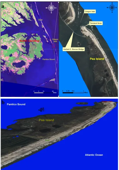
Oregon Inlet is located at the North Carolina Outer Banks between Bodie Island to the North and Pea Island to the south (Figure I-3.1). Our study area extends from the north end of Pea Island for a distance of approximately 6 miles to the south. Oregon Inlet is a naturally migrating inlet that over a period of 126 years has migrated south at an average rate of 23 m/yr and receded to the west at an average rate of 5 m/yr (Overton et al., 2004). In 1989, a terminal groin was built to stabilize the north end of Pea Island and to protect the Bonner Bridge. As to determine if the construction of the terminal groin has been increasing the rate of erosion on the downdrift side, aerial photography is taken every two months and ground surveys are conducted at several transect locations twice a year since then. Result show that no significant erosion above background rates have occurred within the first 5 miles south of Oregon Inlet (e.g., Overton and Fisher, 2004).
Figure I-3.1: Study area: a. Location; b. 3-D overview.
a
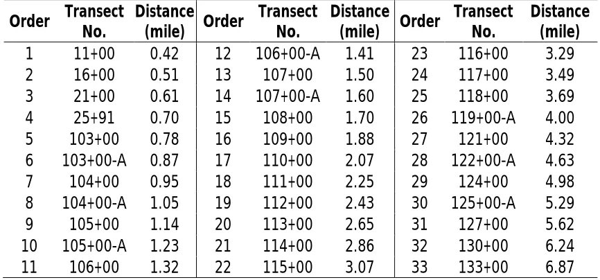
Table I-3.1: Survey transect number with corresponding order number.
Order Transect No. Distance (mile) Order Transect No. Distance (mile) Order Transect No. Distance (mile)
1 11+00 0.42 12 106+00-A 1.41 23 116+00 3.29
2 16+00 0.51 13 107+00 1.50 24 117+00 3.49
3 21+00 0.61 14 107+00-A 1.60 25 118+00 3.69
4 25+91 0.70 15 108+00 1.70 26 119+00-A 4.00
5 103+00 0.78 16 109+00 1.88 27 121+00 4.32
6 103+00-A 0.87 17 110+00 2.07 28 122+00-A 4.63
7 104+00 0.95 18 111+00 2.25 29 124+00 4.98
8 104+00-A 1.05 19 112+00 2.43 30 125+00-A 5.29
9 105+00 1.14 20 113+00 2.65 31 127+00 5.62
10 105+00-A 1.23 21 114+00 2.86 32 130+00 6.24
11 106+00 1.32 22 115+00 3.07 33 133+00 6.87
Note: the distance is referenced to the tip of the Terminal Groin of Oregon Inlet.
3.2 Data collection
The data used in this study covers the period from October 1989 to April 2009. The survey data is collected every six months by NCDOT (North Carolina Department of Transportation). Additional data used is downloaded from public domain sources and data collection agencies, such as tide station, wave gauge stations.
(1) Flight time data
The flight time associated with the shoreline is used to determine both of the wave and tide conditions. The most flights were conducted between 10am and 2pm on a survey day. For the unavailable fight time, we use 12:00pm as the default time to look up the correct wave and tide conditions.
(2)Tide data
interval of 6 min. All tide data used in this study was based on the time when the aerial photos were taken, based on MTL (Mean Tidal Level) datum in meter.
(3) Wave data
The wave data used in this study comes from two sources, which are the WIS (Wave Information Studies) data and wave gauge data, including significant wave height, peak wave period and averaged wave direction, as well as the wind speed and direction, with a constant sample rate of one hour. The WIS data is generated by numerical simulation of past wind and wave conditions, a process called hindcast. Due to the availability of WIS data, only the time period from 1989 to 1999 at Station #222 was used in this study to characterize the wave conditions, which is located at Lat/Lon of 35.92/-75.42 with a depth of 19 m. In addition to WIS data, the wave gauge data was used as a backup source and was retrieved from NOAA buoy station #44014 for the period from 2000 to 2009, for the wave gauge data does not have a good availability before 2000. This station is located at Virginia Beach in VA (36°36'40" N, 74°50'11" W) with a water depth of 47.5 m. The wave data from two sources were collected based on the time when the actual aerial photos were taken.
(4) Shoreline data
The shoreline data are retrieved from the combination of T-sheet and aerial photos in means of wet/dry shoreline, collected by NCDOT. It delineates the contact of land and the water and reflects the position of water/land contact at that moment. The shoreline data used in this study includes the historical shoreline GIS vector data from October 1989 to April 2009 in April and October for each year, which are totally 40 datasets.
(5) Beach profile data
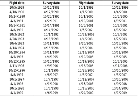
of beach surveys are approximately consistent with the airplane flight dates, with a few exceptions (Table I-3.2). It is assumed that the differences between the two dates will not result in topographic changes.
Table I-3.2 Comparison between beach survey dates and airplane flight dates
Flight date Survey date Flight date Survey date
10/5/1989 10/10/1989 10/1/1999 10/13/1999
4/18/1990 4/17/1990 4/1/2000 4/4/2000
10/24/1990 10/25/1990 10/1/2000 10/3/2000
4/3/1991 4/2/1991 4/10/2001 4/9/2001
10/14/1991 10/14/1991 10/5/2001 10/9/2001
4/8/1992 4/14/1992 4/5/2002 4/3/2002
10/3/1992 10/1/1992 10/22/2002 10/8/2002
4/28/1993 4/13/1993 4/4/2003 4/7/2003
10/4/1993 10/11/1993 9/26/2003 10/15/2003
4/14/1994 4/15/1994 4/6/2004 4/5/2004
10/28/1994 10/11/1994 12/13/2004 10/11/2004
4/5/1995 4/4/1995 4/19/2005 4/5/2005
10/12/1995 10/10/1995 10/19/2005 10/3/2005
4/11/1996 4/9/1996 4/13/2006 4/11/2006
10/15/1996 10/1/1996 10/25/2006 10/10/2006
4/8/1997 4/8/1997 4/3/2007 4/3/2007
10/1/1997 10/7/1997 10/12/2007 10/10/2007
4/1/1998 4/1/1998 4/15/2008 4/9/2008
10/1/1998 10/6/1998 10/15/2008 10/14/2008
4/1/1999 4/6/1999 4/24/2009 4/1/2009
4
Methods
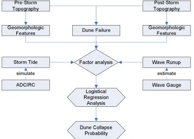
With the description and definition of shoreline above, the elevation of the wet/dry shoreline can be modeled as a function of the “real” shoreline level, tide level and wave runup level. As a result, the “real” shoreline can be exposed by removing the tide and wave runup factors. Finally, the rectified shoreline can reflect the geomorphology changes alongshore caused by the sediment transport process, but not due to wave or tide level changes.
4.1 Shoreline rectification
Figure 4-1 below provides a flow chart of the procedure to remove the horizontal displacement of the shoreline due to the presence of waves and tides at the time of the aerial photography. In order to estimate the “real” shoreline, the tide and wave effects should be removed. The tide level can be easily obtained from the records at tide stations, while the wave runup can be well estimated through the techniques of runup computation by knowing the foreshore slope and deep-water wave conditions. The total vertical shift from the “real” shoreline to the wet/dry shoreline can be assumed to be the summation of tide level (MTL) and wave runup. Finally, the “real” shoreline can be estimated by eliminating the effects of the tide level and wave runup. This methodology was applied to all transects overt the 20-year study period.
4.1.1 Tide estimation
The tide level is not a constant over time, but fluctuates from time to time due to the rotation of the earth. Since the wet/dry shoreline was digitized based on the orthophotos, we use the previous high tide level on the date before the orthophoto was taken, which is based on the Mean Tidal Level (MTL).
4.1.2 Wave runup computation
Recall the runup equation (2.8), three variables need to be obtained before it can be estimated, which are the foreshore slope, deep-water wave height (H0) and wave length (L0). The foreshore slope will be extracted from the beach profile data, while the deep-water wave height and wave length will computed via linear wave theory based on the data provided by the wave gauges.
(1) Foreshore slope
The beach profile extends from NC 12 to approximately MLW (Mean Low Water). The foreshore slope βf was computed based on the end section of the beach profile, which is approximately between MHW and MLW. The elevation were extracted and the foreshore slope was computed automatically at 33 survey transects for 40 datasets from October 1989 to April 2009.
(2) Deep-water wave conditions
The deepwater wave height H0 was computed from the collected wave data via linear wave theory, but only considered the shoaling (dispersion relation) and refraction (Snell’s Law) processes, i.e., the deep-water wave height H0 is a function of refraction coefficient KR,
shoaling coefficient KS, and wave height at reference points Href.
0 R S ref
H =K K H
The deep water wave length L0 is formulated by the equation L0 =gT2/ 2π , which is only a
function of peak wave period. Both computations of wave parameters are based on wave conditions at the flight time on the day.
(3) Wave runup estimation
Given the foreshore slope βf, deep-water wave height H0 and wave length L0, the 2%
exceedence wave runup was computed for 33 transects of total 40 time points based on the following equation (Stockdon, 2006).
2 1/ 2
0 0 1/ 2
2 0 0
[ (0.563 0.004)] 1.1 0.35 ( )
2 f f
H L
R = β H L + β +
(4.2) It is noticed that the 2% exceedence wave runup is a monotone increasing function of βf, H0 and L0, which means that higher wave height, longer wave length or steeper foreshore slope
will elevate the wave runup and cause erosion to the beach region. Finally, the estimated wave runup will be used as the wave effect on the shoreline rectification.
4.1.3 Wet/dry shoreline rectification
Finally, the computed biased term needs to be applied to all wet/dry shoreline, as to get the rectified shoreline data. Thus, Linear Referencing (LR) was applied to achieve this purpose. LR is a technique of recording geographic locations by using relative positions along a measured linear feature. In this study, we firstly define the origin at each survey transect and compute the relative location of the original shoreline to the origin. Then, apply LR technique to rectifying shoreline position along each survey transect based on the computed horizontal shoreline shift. Last, convert the relative shoreline position into ordinary position in original coordinate system. As a result, the rectified shorelines were created and wave/tide effects have been removed.
4.2 Shoreline change analysis
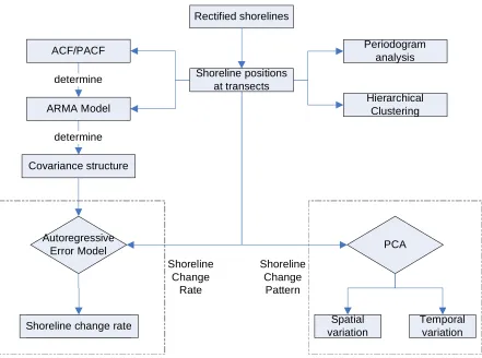
Before the shoreline change analysis can be performed, all the shoreline positions are recorded as distances measured from a fixed reference line offshore. In this case, an increase in distance indicates erosion and a decrease in distance indicates accretion. To characterize the shoreline change, both shoreline change pattern and change rate are considered in the analysis.
Rectified shorelines
Shoreline positions at transects
Autoregressive Error Model
ACF/PACF
determine
Covariance structure determine
Shoreline change rate
Shoreline change rate ARMA Model
Periodogram analysis
Shoreline Change
Rate
Hierarchical Clustering
PCA
Spatial variation
Temporal variation Shoreline
Change Pattern
Figure I-4.2: Shoreline change analysis procedure.
4.2.1 Shoreline change pattern
(1) Analysis of temporal dependency
(2) Parameterization of ARMA model
The ARMA model is usually used to model and quantify the temporal correlation existing in the residuals, though its major purpose is for forecasting data. Before an ARMA model can be applied to any time series data, its AR and MA components must determined. The most commonly used method is to compute the ACF/PACF to see whether it tails off or cut off when the lag increases. The preliminary results suggest that ACF for all transect tails off with sinuous or cosine pattern, while most of PACF cuts off after lag 1 or lag 2. As a result, AR(2) should be the most appropriate model to capture the covariance structure of the residuals. (3) Shoreline change periodicity
Periodogram analysis is used to identify the periodicity existing in the data residuals. It is necessary to perform the periodogram analysis, if the estimated ACF has shown a sinuous or cosine pattern. The temporal trend has to be removed before the periodogram analysis was performed. The spectral power was computed for each transect location and the frequencies with significant spectral power are the associated periodicities for the corresponding time series shoreline data.
(4) PCA analysis and hierarchical clustering
As to capture the shoreline change pattern, the agglomerative hierarchical clustering technique was applied to the shoreline change data. The BIC (Bayesian Information Criterion) was computed before the clustering, to decide the number of categories. The maximum BIC determines the best categories and clustering model for the data. Finally, the average linkage method was used to compute the distance between clusters, and the dendrogram was plotted as to see the structure of the hierarchical clusters.
4.2.2 Modeling shoreline change rate
5
Result
5.1 Wave runup and shoreline shift
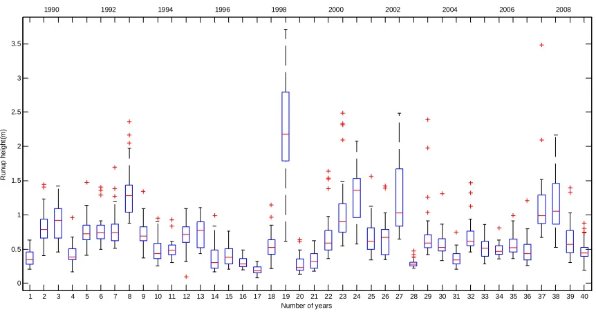
The averaged wave runup over transects for each year is shown below (Figure I-5.1). It is clear to conclude that almost all the wave runups are between 0.2 m and 2.5 m, while most of them are below 1.5 m, with the exception in October, 1998, which is due to both higher H0 and longer waver period on photo taken date. In addition, the spatial variation of wave runup over difference transects exists due to the spatial variation of foreshore slope.
Finally, the estimated horizontal shoreline shifts based on the wave runup and tide level were applied to the rectification of the shorelines. The results suggest the averaged horizontal shift of shoreline over transects for each year is between 5 m and 10 m with a few exceptions, such as October 1999, in which the averaged horizontal shift is -7.42 m, for the tide level during the flight time is relative low (-0.46 m).
Figure I-5.1: Estimation of averaged wave runup over transects for each year.
1 2 3 4 5 6 7 8 9 10 11 12 13 14 15 16 17 18 19 20 21 22 23 24 25 26 27 28 29 30 31 32 33 34 35 36 37 38 39 40 0
0.5 1 1.5 2 2.5 3 3.5
R
u
n
up
h
e
ig
h
t(
m)
Number of years
5.2 Shoreline change pattern
(1) ACF of shoreline data residuals
0 5 10 15 20 -0 .4 0 .0 0 .4 0 .8 Lag A CF
ACF of Residuals at Transect #5
0 5 10 15 20
-0 .4 -0 .2 0 .0 0 .2 Lag P a rt ia l A CF
PACF of Residuals at Transect #5
0 5 10 15 20
-0 .5 0 .0 0 .5 1 .0 Lag A CF
ACF of Residuals at Transect #10
0 5 10 15 20
-0 .2 0 .0 0 .2 0 .4 Lag P a rt ia l A CF
0 5 10 15 20 -0 .2 0 .2 0 .6 1 .0 Lag A CF
ACF of Residuals at Transect #15
0 5 10 15 20
-0 .2 0 .0 0 .2 0 .4 Lag P a rt ia l A CF
PACF of Residuals at Transect #15
0 5 10 15 20
-0 .2 0 .2 0 .6 1 .0 Lag A CF
ACF of Residuals at Transect #20
0 5 10 15 20
-0 .3 -0 .1 0 .1 0 .3 Lag P a rt ia l A CF
0 5 10 15 20 -0 .2 0 .2 0 .6 1 .0 Lag A CF
ACF of Residuals at Transect #25
0 5 10 15 20
-0 .3 -0 .1 0 .1 0 .3 Lag P a rt ia l A CF
PACF of Residuals at Transect #25
0 5 10 15 20
-0 .2 0 .2 0 .6 1 .0 Lag A CF
ACF of Residuals at Transect #30
0 5 10 15 20
-0 .3 -0 .1 0 .1 0 .3 Lag P a rt ia l A CF
(2) Shoreline change periodogram
0.2 0.4 0.6 0.8 1.0 0 1 0 000 3 0 000 frequency s pe c tr um
Periodogram at Transet #5
bandwidth = 0.0144
0.2 0.4 0.6 0.8 1.0
0 1 0 000 3 0 000 frequency s pe c tr um
Periodogram at Transet #10
bandwidth = 0.0144
0.2 0.4 0.6 0.8 1.0
0 50 00 1 50 00 frequency s pe c tr um
Periodogram at Transet #15
0.2 0.4 0.6 0.8 1.0 1 0 00 2 000 3 000 40 00 frequency s pe c tr um
Periodogram at Transet #20
bandwidth = 0.0144
0.2 0.4 0.6 0.8 1.0
0 1 000 20 00 30 00 frequency s pe c tr um
Periodogram at Transet #25
bandwidth = 0.0144
0.2 0.4 0.6 0.8 1.0
0 5 00 1 000 2 000 frequency s pe c tr um
Periodogram at Transet #30
(3) Principal components of shoreline changes a. Taking transects as variables
Figure I-5.4 shows the plot of eigenvalues, named as the scree plot, for which the PCA was performed by taking the locations as multiple variables. The scree plot suggests that the first principal component can explain the most of the variance for all years. The computation also shows that 50.9% of the total variance can be explained by the first principal component, and 75.3% of the total variance can be explained by the first four principal components.
Figure I-5.4: Scree plot for the PCA on transects of shoreline change data.
Figure I-5.5 has clearly shown that the shoreline changes oscillate intensively for the first 20 transects (about 2.65 miles from the Oregon Inlet), relative to the last 13 transects, based on the eigenvectors of the first four principal components. By looking at only the eigenvector of the first principal component, negative values indicate that the shoreline accretion dominated the whole shoreline evolution process during the past 20 years, while the first 20 transects,
0 5 10 15 20 25 30
0
20
00
4
000
6
0
00
80
00
10
0
00
1
20
00
1
4
0
00
Index
la
m
b
which are about 2.65 miles from the Oregon Inlet, had more accretion as compared with the last 13 transects.
Figure I-5.5: The eigenvectors of the first four components versus distant alongshore.
In addition to the eigen-vectors of principal components, the first principal component was also plotted as below (Figure I-5.6), which can explain 50.9% of the total variance. Four extraordinary points were marked due to some special events happened associated with them. By looking at the storm historical records, Hurricane Emily, Dennis, and Isabel, occurred in September 1993, September 1999 and September 2003 respectively. These storm events are the best indicators which can be used to explain the great shoreline recession in those years (event 1, 2 and 3, positive value means shoreline erosion). Moreover, event 4 has shown a shoreline accretion in 2004 (negative value means shoreline accretion). By looking at beach projects, nourishment project has been implemented and a huge amount of sand (1.03 million cubic yard) was placed in October 2004, which can well explain why a big shoreline accretion is detected in between 2003 and 2004.
1 2 3 4 5 6 7
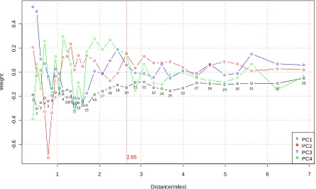
-0 .6 -0 .4 -0 .2 0 .0 0 .2 0 .4 Distance(miles) We ig ht PC1 PC2 PC3 PC4 1 2 3 4 5 67 8 9 101112 1314 15 16 17 18 19 20 21 22 23 24 25 26
27 28 29 30 31 32
33
Figure I-5.6: The geographic locations of the beach nourishment projects.
Figure I-5.7 below is showing the major beach nourishment projects implemented during the past 20 years. The horizontal lines represent the geographic region covered by the beach nourishments, measured by distance from the Terminal Groin of Oregon Inlet. The locations of beach nourishment projects are very consistent with the spatial principal components, i.e., the locations which have larger weights are the places where the beach nourishment was conducted. As a result, the beach nourishment project is one of the major factors causing the intensive oscillation of shoreline changes.
Year C omp o s it e S ho re li n e C ha n ge (m /s e m i-y e a r)
1990 1995 2000 2005
-200 -100 0 100 200 300 1 2 3 4
Figure I-5.7: The geographic locations of the beach nourishment projects.
b. Taking times as variables
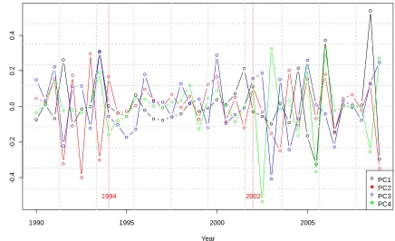
Figure I-5.8 shows the scree plot, for which the PCA was performed by taking times as multiple variables. It is clear to see that the first four principal components explain the most of the total variance, though the first principal component does not significantly explain the most of the total variance. The computation shows that 20.7% of the total variance can be explained by the first principal component, and 59.3% of the total variance can be explained by the first four principal components.
1992
1993
1995 2001 2001
2002 2003
2004 2004 2008
2009
2.65 2.65
0 0.2 0.4 0.6 0.8 1 1.2 1.4
0 1 2 3 4 5 6 7
Sa
nd
V
ol
um
e
(m
illi
on
c
ub
ic
y
ar
d)
Figure I-5.8: Scree plot for the PCA on times of shoreline change data.
Figure I-5.9 shows the eigenvectors of the first four components versus year. The magnitudes of the eigenvectors elements suggest that the variations of shoreline changes are less dependent on the period from 1994 to 2002, which means that the shoreline changes were relatively small during the period from 1994 to 2002, while that is higher before 1994 and after 2002. In addition, the shoreline changes after year 2002 were a little bit higher than that before year 1994.
0 10 20 30 40
0
1
0
00
2
000
30
00
Index
la
m
b
Figure I-5.9: The eigenvectors of the first four components versus year.
Figure I-5.10 is showing the historical records of the beach nourishment projects, as well as big storms. It suggests the volume of disposal sand is relative small during the period from 1994 to 2002, but relative high during the period before 1994 and after 2002. This result is also consistent with the temporal principal components, i.e., the years which have less weights in the principal components are the years when smaller amount of sand was nourished. Therefore, the beach nourishment projects may be the major factors causing the shoreline changes. In addition, the dates of a few big storm events are also consistent with some higher oscillations of the eigenvectors of the principal components, especially for the year 2003. As result, the storm event is probably another important factor causing the shoreline changes.
1990 1995 2000 2005
-0
.4
-0
.2
0
.0
0
.2
0
.4
Year
W
e
ig
ht
PC1 PC2 PC3 PC4
Figure I-5.10: The history records of the beach nourishment projects and storms.
(4) Shoreline changes clustering
By running model selection function (Mclust) for hierarchical clustering, we get the maximum BIC of -11699.14, which suggests “ellipsoidal, equal volume, shape, and orientation” model with 6 clusters. As a result, we divide all the shoreline change styles based transects into 6 categories. Figure I-5.11 shows the dendrogram of the cluster, which suggests that last 27 transects have similar shoreline change patterns.
1994 2002
1992 1994 1995 1998 1999 2003 2004 2005 2007 2008 2009 1991
0 0.2 0.4 0.6 0.8 1 1.2 1.4 1.6 1.8
1990 1992 1994 1996 1998 2000 2002 2004 2006 2008 2010
Sa
nd
V
ou
m
ne
(m
ill
ion
c
ub
ic
y
ar
d)
Figure I-5.11: Cluster dendrogram for the shoreline change data.
5.3 Shoreline change rate
The Figure I-5.12 below shows the shoreline change rate for each transect during the period from 1989 to 2009, in which positive rate refers to erosion, and negative rate refers to accretion. The spatial variation of shoreline change rate exposed different change patterns affected by the geomorphologic properties from the Oregon Inlet to its south. It is clear to see that the general spatial trend of shoreline change rate are quite similar derived by both OLS and AEM methods. From the Oregon Inlet to its south, the shoreline change rate increases till the transect #12, and then decreases till transect #15. From transect #16 to #23, shoreline change rate remain approximately the same. From transect #24 to #33, the shoreline change rate goes up and down. Since the positive rate means erosion and negative rate means accretion, the shoreline change pattern has a general trend of increasing erosion when it goes from the Oregon Inlet to its south. However, the estimated shoreline change rate by AEM is almost always below that by the OLS regression method, which means that OLS regression method has over estimated the shoreline erosion rate, by ignoring the temporal correlation in the shoreline data. As a result, to simply apply the OLS method to the estimation of linear rate will mislead to the wrong change pattern of the shorelines.
5 6
11 12 14 10 13 15 9 16 7 8 19 17 18 29 24 25 20 22 23 31 28 26 21 30 27 32 33 3 4 1 2
50
100
150
200
250
Cluster Dendrogram
hclust (*, "average") Transect
H
e
Figure I-5.12: The comparison of shoreline change rates between the OLS and AEM methods.
The Figure I-5.13 below shows the estimate parameters for AR terms with their associated p-values. Almost all the factors for the AR term are negative, which means the residual terms of current shoreline positions are always decreased by the previous ones, i.e., those unknown factors cause accretion to the shorelines. By looking at the p-values, the significant AR(1) process appears between the transect #5 to #10 and #20 to #25, while the significant AR(2) only appears between transect #10 to #15. Therefore, those unknown factors affected shoreline position mostly at a lag of a half year.
0 1 2 3 4 5 6 7
-3 -2 -1 0 1 2 3 4 1 2 3
4 5 6 7 8 9 10 11 12 13 1415 16 17 18
19 20 21
Figure I-5.13: The estimated parameters for the AR terms and their associated p-values.
-0.8 -0.6 -0.4 -0.2 0.0 0.2 0.4 0.6 0.8 1.0 1.2
0 5 10 15 20 25 30 35
Co
effi
ci
ent
Transect Number
6
Discussion
In this study, the shoreline change pattern and rate were analyzed by considering both wave/tide effects and statistical models. The wave runup or tide fluctuation may cause an instant water level shift, which results in wet/dry shoreline shift consequently. The statistical models have been applied to the rectified shoreline data, in order to capture the shoreline change pattern and rate, and finally can be used for prediction.
(1) Wave / tide effects
To remove the wave/tide effects, the wet/dry shoreline were firstly rectified by computing the wave runup and tide level, in which the waves result in water level raise due to wave runup, while the tide causes a water level raise directly. It is assumed that the rectified shoreline is more closed to the “actual” shoreline due to the removal of wave/tide effect. However, the estimated wave runup may not exactly reflect the actual wave runup, which results in the wet line alongshore.
(2) Capturing shoreline variation
The PCA has extracted the structure of the shoreline change variations. In the means of both spatial and temporal view, the special pattern of shoreline change variations was exposed distinctly and well explained by the beach nourishment activity and the storm events qualitatively. However, the magnitude of shoreline change variations may need to be further discussed by correlating with the beach nourishment volume and the storm index, in order to address how the beach nourishment and storm events change the shoreline quantitatively. (3) Estimation of shoreline change rate
confidence intervals for the predicted values are not correct. Second, the estimations of the regression coefficients are not as efficient as they would be if temporal dependency is taken into account. Finally, since the residuals of OLS regressions are not independent, the additional information in the residuals, temporal dependency, needs to be further extracted as to capture more data variations.
The AEM solves this problem by improving the regression model through adding an autoregressive model for the autocorrelation of the errors. As a result, both temporal trend and dependency can be captured, and the regression estimates was corrected for autocorrelation by the AEM method. In our study case, the improvement of model performance is measured by AIC (Akaike’s Information Criterion). The minimum AIC specifies the best model. Figure I-6.1 shows the decreased AIC from OLS to AEM, and their associated p-values for AR terms. The vertical blue lines indicate decreased AIC from OLS to AEM. It is clear to see that, as long as there is a decrease in AIC from OLS to AEM, the associated p-value of at least one of the AR terms will be significant (Figure I-6.1). Finally, it is suggested that AEM improves the parameter estimation for the first 3 miles.
Figure I-6.1: Increased AIC from OLS to AEM, as well as the associated p-values for AR terms.
0 1 2 3 4 5 6 7
0.00 0.05 0.10 0.15 0.20 0.25
Distance(mile)
M
a
g
n
it
u
d
e
o
f
v
a
ri
ab
les
Figure I-6.2: Comparison of modeling shoreline data: a. OLS regression; b. AEM.
a
7
Conclusion
Chapter 2 Vulnerability Analysis of Coastal Dunes due to
Short-Term Storm Effect through Geomorphology Features
Abstract