University of Windsor University of Windsor
Scholarship at UWindsor
Scholarship at UWindsor
Electronic Theses and Dissertations Theses, Dissertations, and Major Papers
2014
A case study of integrated modelling of traffic, vehicular
A case study of integrated modelling of traffic, vehicular
emissions, and air pollutant concentrations for Huron Church
emissions, and air pollutant concentrations for Huron Church
Road, Windsor
Road, Windsor
Hassan Mohseni Nameghi
University of Windsor
Follow this and additional works at: https://scholar.uwindsor.ca/etd
Recommended Citation Recommended Citation
Mohseni Nameghi, Hassan, "A case study of integrated modelling of traffic, vehicular emissions, and air pollutant concentrations for Huron Church Road, Windsor" (2014). Electronic Theses and Dissertations. 5069.
https://scholar.uwindsor.ca/etd/5069
A case study of integrated modelling of traffic, vehicular emissions, and air pollutant concentrations for Huron Church Road, Windsor
by
Hassan Mohseni Nameghi
A Dissertation
Submitted to the Faculty of Graduate Studies through Civil and Environmental Engineering in Partial Fulfillment of the Requirements for
the Degree of Doctor of Philosophy at the University of Windsor
Windsor, Ontario, Canada
2013
A case study of integrated modelling of traffic, vehicular emissions, and air pollutant
concentrations for Huron Church Road, Windsor
by
Hassan Mohseni Nameghi
APPROVED BY:
______________________________________________ Dr. Ashok Kumar, External Examiner
Department of Civil Engineering, The University of Toledo ____________________________________________
Dr. Bill Anderson, Outside Reader Department of Political Science
______________________________________________ Dr. Paul Henshaw, Department Reader
Department of Civil and Environmental Engineering ______________________________________________
Dr. Rajesh Seth, Department Reader
Department of Civil and Environmental Engineering ______________________________________________
Dr. Xiaohong Xu, Advisor
Department of Civil and Environmental Engineering ______________________________________________
Dr. Chris Lee, Co-Advisor
Department of Civil and Environmental Engineering ______________________________________________
Dr. Stephen Brooks, Chair of Defense Department of Political Science
iii
DECLARATION OF ORIGINALITY
I hereby certify that I am the sole author of this thesis and that no part of this thesis has
been published or submitted for publication.
I certify that, to the best of my knowledge, my thesis does not infringe upon anyone’s
copyright nor violate any proprietary rights and that any ideas, techniques, quotations, or
any other material from the work of other people included in my thesis, published or
otherwise, are fully acknowledged in accordance with the standard referencing practices.
Furthermore, to the extent that I have included copyrighted material that surpasses the
bounds of fair dealing within the meaning of the Canada Copyright Act, I certify that I
have obtained a written permission from the copyright owner(s) to include such
material(s) in my thesis and have included copies of such copyright clearances to my
appendix.
I declare that this is a true copy of my thesis, including any final revisions, as approved
by my thesis committee and the Graduate Studies office, and that this thesis has not been
iv ABSTRACT
The objectives of this research are to examine spatial and temporal variations in
traffic-related NO2 and benzene concentrations and to investigate the sensitivity of estimated
vehicular emissions and ambient concentrations on input parameters. The case study was
conducted for Huron Church Road (9.5 km) in Windsor, Ontario. Observed vehicle
counts and emission factors from Mobile6.2 were used to estimate vehicular emissions.
Ambient concentrations were estimated using the AERMOD dispersion model.
Results showed that traffic on Huron Church Road significantly contributes to
near-road air quality. The simulated annual mean NO2 concentration of 2008 was 27 µg/m3 at 40 m from the road, which was higher than the background concentration of 21
µg/m3. Concentrations sharply decreased with distance from the road. At 600 m from the road, the simulated annual concentration was 9% of the concentrations at a distance of 40
m from the road (=2.4 µg/m3, less than background concentration). Similar patterns were observed for benzene.
Ambient concentrations were higher during the nighttime than the daytime due to
poor mixing. Traffic counts and wind speed explained 40% of variations in the both
observed and simulated NO2 concentrations. The relationship between the truck/car
counts and NO2/benzene concentration ratios was linear.
The model-measurement comparison showed that Mobile6.2 and AERMOD
reasonably reproduced the hour-of-day variations and spatial fall-off pattern of NO2
concentrations. However, AERMOD underestimated concentrations during the daytime
potentially due to over-mixing.
v
sensitive to the choice of Vehicle Mile Traveled compositions (Ontario versus US),
followed by the choice of vehicle age distribution (Ontario versus US), and the average
speed of vehicles. In AERMOD simulations, the hour-of-day variation in emission should
be considered.
Stop-and-go movements increased the total NOx emission over the 9.5 km road
by 24% compared to the case of cruise speed of 50km/h during the morning peak hour.
Two correction (multiplication) factors were devised to adjust uniform emissions by
Mobile6.2 near signalized intersections: an upstream correction factor of 3.2 to account
for idling and acceleration emissions, and a downstream correction factor of 1.6 to
DEDICATION
ACKNOWLEDGEMENTS
I would like to sincerely acknowledge all who supported my Ph.D. research at University
of Windsor. In particular, my special thanks to my advisors, Dr. Xiaohong Xu and Dr.
Chris Lee, for supervision, financial support and giving me the opportunity to learn and
to grow, to think critically, to write professionally, and to manage the time wisely. I
would like to thank my committee for providing great insights towards my research: Dr.
Paul Henshaw, Dr. Bill Anderson, and Dr. Rajesh Seth from University of Windsor and
Dr. Ashok Kumar from The University of Toledo. I would like to thank Dr. Amanda
Wheeler from Health Canada for providing valuable and insightful suggestions and Mr.
John Wolf from City of Windsor for providing Windsor vehicle counts used in this study.
I acknowledge Health Canada for providing average NO2 concentrations at 11 sites near
Huron Church Road used for validation of fall-off patterns.
I would like to acknowledge the University of Windsor and the Ontario Ministry
of Education for scholarships. Funding for the research contained in this dissertation was
provided by Health Canada and the Natural Sciences and Engineering Research Council
viii
TABLE OF CONTENTS
DECLARATION OF ORIGINALITY ... iii
ABSTRACT ... iv
DEDICATION ... vi
ACKNOWLEDGEMENTS ... vii
LIST OF TABLES ... xii
LIST OF FIGURES ... xvi
1. INTRODUCTION 1 1.1 Background ...1
1.2 Objectives ...6
1.3 Organization of thesis ...7
2. REVIEW OF LITERATURE 8 2.1 Atmospheric dispersion models ...8
2.2 Vehicular emission models ...14
2.3 Selection of dispersion and emission models ...17
2.4 Relationship between NO2 and benzene concentrations ...18
2.5 Limitations in the current literature ...22
2.5.1 Vehicle counts ... 22
2.5.2 Vehicular emissions ... 24
2.5.3 Air pollutant concentration ... 28
3. METHODOLOGY 30 3.1 Integrated traffic and air quality modeling ...30
3.2 Vehicle count data ...31
3.2.1 City of Windsor intersection counts ... 34
3.2.2 City of Windsor hourly counts ... 34
3.2.3 DRIC mid-block counts ... 35
3.2.4 DRIC hourly counts ... 35
3.2.5 Windsor-Detroit US entry counts ... 35
3.3 Estimation of vehicle counts for spatial variations ...36
3.3.1 Adjusting City of Windsor intersection counts ... 36
3.4 Spatial and temporal distribution of vehicle counts ...39
3.4.1 Spatial distribution ... 39
3.4.2 Temporal distribution ... 41
3.5 Estimation of NOx and benzene emission factors...43
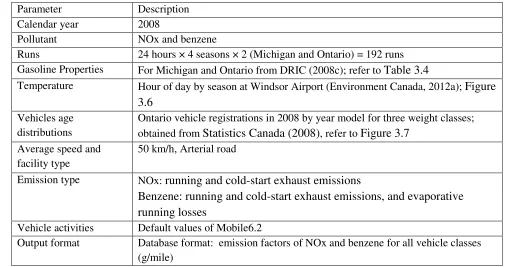
3.5.1 Mobile6.2 setup parameters ... 43
3.5.2 Fuel properties ... 47
3.5.3 Vehicle age distribution ... 50
3.5.4 Estimation of composite emission factors ... 51
3.6 Estimation of NO2 and benzene concentrations ...54
3.6.1 AERMOD simulation setup ... 55
3.6.2 Analysis of simulation results ... 61
3.6.3 Relationship between NO2 /benzene and truck/car ratios ... 70
3.7 Effects of input parameters on estimated emissions and concentrations ...72
3.7.1 Sensitivity of results to input data in a macroscopic level using Mobile6.2 and AERMOD ... 72
3.7.2 Options in AERMOD ... 86
3.7.3 Effect of stop-and-go movement in a microscopic level ... 93
3.7.3.1 Study area ...94
3.7.3.2 Description of Scenarios ...95
3.7.3.3 Spatial distribution of average speed and SAFD ...97
3.7.3.4 Vehicular emission ...107
3.7.3.5 Correction factors for NOx emissions by Mobile6.2 near signalized intersections ...112
3.7.3.6 NO2 simulation ...114
4. RESULTS OF PART I: SPATIAL AND TEMPORAL DISTRIBUTIONS OF VEHICLE COUNTS, EMISSIONS AND CONCENTRATIONS 116 4.1 Vehicle counts ...116
4.1.1 Long-term variations in vehicle counts ... 116
4.1.2 Spatial patterns of vehicle counts ... 118
4.1.3 Temporal patterns of vehicle counts ... 122
4.2 Temporal patterns of NOx and benzene emission factors ...125
4.3 NOx and benzene emissions ...127
4.3.1 Spatial patterns of emissions ... 127
4.3.2 Temporal patterns of emissions ... 129
4.4 Patterns of meteorological factors ...130
4.4.1 Annual and seasonal wind-roses ... 130
... 132
4.5 Spatial and temporal patterns of NO2 and benzene concentrations133 4.5.1 Spatial patterns of concentrations ... 133
4.5.2 Falloff patterns of concentrations ... 135
4.5.3 Temporal patterns of concentrations ... 138
4.5.3.1 Effects of meteorological parameters and vehicle types on hour-of-day concentrations ...140
4.5.3.2 Comparison of simulated and observed concentrations ..147
4.5.4 Major factors affecting NO2 concentrations ... 153
4.6 Regression models of concentrations ...161
4.6.1 Hourly concentration models ... 161
4.6.2 Annual mean concentration models ... 166
4.7 Ratio of NO2 to benzene concentrations ...168
4.7.1 Spatial distribution of NO2/bezene concentration ratios ... 168
4.7.2 Relationship between ratio of simulated NO2/benzene and truck/car ratio ... 172
4.8 Comparison of simulated and observed NO2/NOx and NO2/benzene ratios 177 4.9 Summary ...182
5. RESULTS OF PART II: EFFECTS OF INPUT DATA ON EMISSIONS AND CONCENTRATIONS 184 5.1 Effects of more-detailed input data in a macroscopic level ...184
5.1.1 Emission factors and total emission ... 184
5.1.2 Spatial distribution of concentrations ... 192
5.1.3 Temporal distribution of concentrations ... 195
5.1.4 Summary ... 202
5.2 Effects of options in AERMOD ...205
5.2.1 Effects of site characteristics ... 205
5.2.2 Options for NO2 simulation ... 210
5.2.3 Comparison of volume and area sources ... 214
5.2.4 Summary ... 216
5.3 Effects of stop-and-go traffic movements in a microscopic level ..217
5.3.1 Stop-and-go profiles ... 217
5.3.2 Vehicular emissions ... 222
5.3.2.1 Micro-emission model ...222
5.3.2.2 Mobile6.2 ...225
5.3.4 NO2 concentration ... 231
5.3.5 Summary ... 236
6. CONCLUSIONS AND RECOMMENDATIONS 239 6.1 Conclusions ...239
6.2 Recommendations ...245
REFERENCES ...249
APPENDICES ...261
Appendix A: Meteorological data source and processing ...261
Appendix B: Results of ANOVA and regression models ...265
Appendix C: Mobile6.2 – Road type and average speed ...267
Appendix D: AERMOD formulation for estimation of turbulence coefficients ...271
Appendix E: Copyright permissions ...274
LIST OF TABLES
Table 2.1: A comparison of six dispersion models ... 9
Table 2.2: A comparison of chemistry modules used in five dispersion models ... 13
Table 2.3: A comparison of evaluated methods for estimating emission factors ... 15
Table 2.4: Observed NO2/benzene ratios in previous studies ... 21
Table 3.1: Traffic data used in this study ... 33
Table 3.2: Vehicle classification by length at two traffic count stations ... 34
Table 3.3: Mobile6.2 setup parameters ... 44
Table 3.4: Average gasoline properties in Michigan and Ontario, collected in 2003 (DRIC, 2008c)... 45
Table 3.5: Average gasoline properties in Ontario and Michigan. ... 49
Table 3.6: Alignment of vehicle age distribution categories in Mobile6.2 and this study ... 50
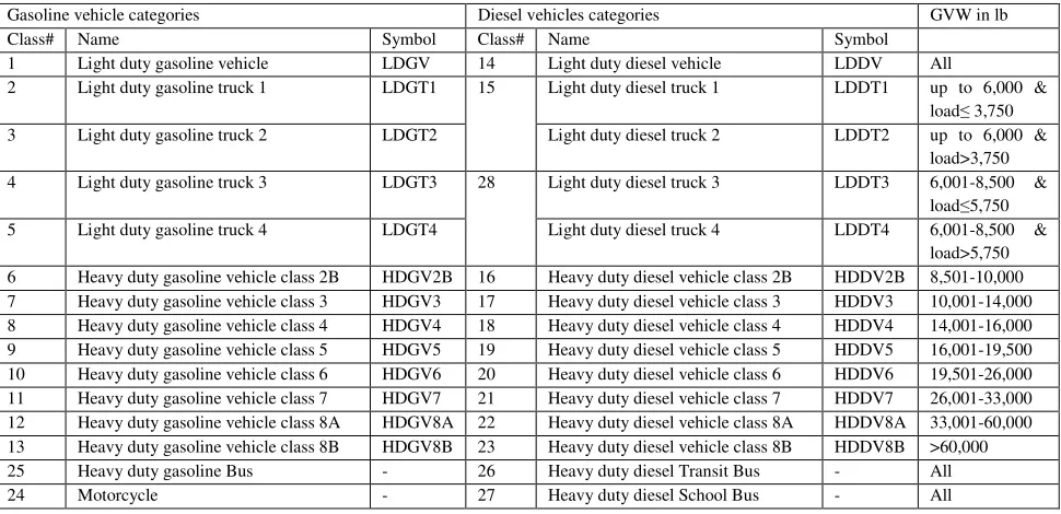
Table 3.7: Vehicle classification in Mobile6.2 (Cook and Glover, 2002) ... 51
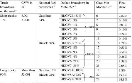
Table 3.8: Mapping car category in vehicle counts with vehicle classes in Mobile6.2 .... 52
Table 3.9: Mapping truck category in vehicle counts with vehicle classes in Mobile6.2 53 Table 3.10: Summary of model setup parameters for dispersion calculation in AERMOD ... 57
Table 3.11: Descriptive statistics of concentrations, vehicle counts and meteorological factors ... 66
Table 3.12: Predictor variables for estimation of annual mean concentrations ... 70
Table 3.13: Explanatory variables for estimation of NO2/benzene concentration ratio ... 72
Table 3.15: Setup parameters of Mobile6.2 in the Base Case ... 75
Table 3.16: Difference in emission factors – vehicle age distributions versus default values in Mobile6.2. ... 80
Table 3.17: Average fuel properties in Ontario in 2003 (DRIC, 2008c) ... 82
Table 3.18: Site characteristics in Scenarios 1-3 ... 89
Table 3.19: Scenarios used to investigate effects of stop-and-go ... 96
Table 3.20: constant and polynomial coefficients of acceleration and deceleration profiles in Figure 3.21 ... 104
Table 3.21: Regression coefficients and lower limit of emission (Source: Panis et al., 2006) ... 108
Table 4.1: Mean, standard deviation, and variance of NO2 concentrations ... 145
Table 4.2: One-way ANOVA (R2) of simulated and observed NO2 concentrations with respect to temporal factors, traffic counts, and meteorological conditions at the Windsor-West Station ... 156
Table 4.3: Pearson linear correlation coefficients between hourly NO2 concentrations at the Windsor West Station, and other factors, sample size of all factors was 2870 158 Table 4.4: Multi-factor ANOVA partitioning (R2 (adj)) of simulated and observed NO2 concentrations at the Windsor-West Station (all factor in the models are significant at p<0.05) ... 159
Table 4.5: Hourly concentration models at the receptor 40m east of the road (Equation 3.7) (p<0.001) ... 162
Table 4.6: Hourly concentration models at the receptor 40m east of the road assuming the
3.7) (p<0.001) ... 163
Table 4.7: Hourly concentration models at the receptor 40m east of the road using
normalized hour-of-day car counts (Equation 4.1) (p<0.001) ... 165
Table 4.8: Hourly concentration models at the Windsor-West Station using
Car-NOx-Equivalent counts and wind speed (Equation 3.7) (p<0.001) ... 165
Table 4.9: Estimated parameters of multiple linear regression models - NO2
concentration. All coefficients and models were statistically significant (p < 0.001).
... 167
Table 4.10: Estimated parameters of multiple linear regression models - Benzene
concentration.All coefficients and models were statistically significant (p < 0.001).
... 167
Table 4.11: Constant and coefficients of multinomial linear regression models –
NO2/Benzene concentration ratio versus truck/car counts ratio (for all models p <
0.001) ... 175
Table 4.12: Estimated background concentrations of NO2, NOx, and benzene at three air
quality stations in Windsor ... 180
Table 4.13: Observed and simulated NO2/NOx and NO2/benzene concentration ratios 181
Table 5.1: NOx and benzene emission factors of LDVs and HDVs in the Base Case ... 184
Table 5.2: Summary of results - change in emission factors, emissions, and ambient
concentrations versus the Base Case [(scenario-base case)/base case*100] ... 204
Table 5.3: Time in different driving modes and average speed on the road ... 218
Table 5.4: Total emission over the 9.5km road using the-micro emission model by
Table 5.5: Total emission over the 9.5km road estimated using Mobile6.2 by direction
and method ... 225
Table 5.6: Mobile6.2 NOx correction factors near signalized intersections by vehicle type
... 228
Table 5.7: Range and average of concentrations (µg/m3) among 550 receptors 40 m and
200 m during morning peak hours (9:00-10:00) of 2008, minimum – maximum
LIST OF FIGURES
Figure 3.1: Illustration of multi-model approach of traffic, vehicular emissions, and air
pollutant concentrations ... 31
Figure 3.2: A sketch of the Talbot and Huron Church Roads, and the location of traffic count stations ... 32
Figure 3.3: Comparisons between DRIC and City of Windsor counts - AM peak in northbound ... 40
Figure 3.4: Comparisons between DRIC and City of Windsor counts - PM peak in southbound ... 41
Figure 3.5: Hour of day car and truck counts at three road sections ... 42
Figure 3.6: Hourly-of-day temperature by season at Windsor Airport in 2008... 45
Figure 3.7: Age distribution of Ontario vehicles (Source: Statistics Canada, 2008) ... 46
Figure 3.8: Sketch of Huron Church Corridor, receptors in a buffer of 1000 m (13 thousand receptors), Note: The star mark denotes the location of the Windsor West air quality station, and the circles are two receptors for hourly simulation. ... 58
Figure 3.9: Sketch of the Huron Church Corridor and location of 50 receptors perpendicular to the road on a typical traverse with a spacing of 40 m and 32 receptors along the road located at the middle of road section and 40 m from the road. ... 58
Figure 3.10: Map of passive monitoring sites (yellow pins) near the Giradot-College road section (Source of base map: Google Earth, 2010) ... 63
Figure 3.11: Classification of receptors with respect to the distance to the road ... 69
... 79
Figure 3.13: Vehicle age distribution in Ontario, Canada, and default Mobile6.2 ... 79
Figure 3.14: Comparison of seasonal variations in temperature between Windsor
(Environment Canada, 2012a) and 100 U.S. cities (Infoplease.com, 2012) ... 81
Figure 3.15: Seasonal fuel properties (a) average of 23 US States (EPA, 1999a) (b)
Ontario (DRIC, 2008c) ... 83
Figure 3.16: Hour of day pattern of vehicle counts ... 84
Figure 3.17: Site characteristics in Scenario 4, average of four seasons. ... 90
Figure 3.18: Comparison of mixing heights between Windsor (estimated using
AERMET) and London (source of data: MOE, 2010) ... 91
Figure 3.19: Duration of intervals for through movement at each signalized intersection95
Figure 3.20: Space and time diagram for a vehicle approaching a signalized intersection
(Source: Akçelik & Besley, 2001) – Reprinted with permission (Appendix D). ... 100
Figure 3.21: Typical acceleration and deceleration profiles of vehicles near signalized
intersections (Source: Akçelik & Besley, 2001) – Reprinted with permission
(Appendix D). ... 103
Figure 3.22: Sketch of stopped vehicles behind the stop line at the end of the red interval
... 105
Figure 3.23: NOx emission rate of vehicles versus speed and acceleration (Source of data:
Panis et al., 2006) ... 109
Figure 3.24: Time distribution of speed and acceleration at three selected driving cycles
(Source of data: EPA, 1997). ... 111
Figure 3.26: Sketch of driving modes of vehicles near signalized intersections ... 113
Figure 4.1: Annual car and truck counts at Windsor border crossing from Canada to U.S. ... 116
Figure 4.2: Monthly truck counts at Windsor border crossing from Canada to U.S. in 2004-2008. (Source: BTS (2009)) ... 117
Figure 4.3: Daily car counts on Huron Church Road by month in 2008 at two traffic count stations. ... 118
Figure 4.4: Adjusted car and truck counts in 2008 during peak hours on Huron Church Road ... 120
Figure 4.5: Annual vehicle counts by road segment in 2008 ... 121
Figure 4.6: Spatial distribution of unidirectional annual vehicle counts in 2008 ... 122
Figure 4.7: Hour-of-day variations of vehicle counts in 2008 ... 123
Figure 4.8: Hour of day benzene emission factor by season from Mobile6.2 ... 126
Figure 4.9: Hour of day NOx emission factor by season from Mobile6.2 ... 127
Figure 4.10: Spatial distribution of vehicular emissions in 2008 ... 128
Figure 4.11: Hour-of-day variations in vehicle counts, and NOx and benzene emissions at the Giradot - College road section in 2008 ... 129
Figure 4.12: Seasonal variations in vehicle counts, and NOx and benzene emissions at the Giradot - College road section in 2008 ... 130
Figure 4.13: Wind-rose at Windsor Airport in 2008 ... 131
Figure 4.14: Wind-roses at Windsor Airport in 2008 by season ... 132
Figure 4.16: Annual mean NO2 and benzene concentrations in 2008 ... 134
Figure 4.17: Maximum hourly concentrations of NO2 and benzene ... 135
Figure 4.18: Fall-off pattern of annual and maximum hourly concentrations from the road
centerline – at (c) and (d), concentrations were normalized to those at 40m east of
the road... 136
Figure 4.19: Falloff patterns of simulated and observed NO2 concentrations at a transit
line perpendicular to the Giradot - College road section in May 2010 – Observed
concentrations were provided by Health Canada... 137
Figure 4.20: Hour of day NO2 and benzene concentrations at a receptor 40 m east and a
receptor 40 m west of the road ... 139
Figure 4.21: Seasonal mean NO2 and benzene concentrations at a receptor 40 m east and
a receptor 40 m west of the road ... 140
Figure 4.22: Hour-of-day concentrations at the Windsor-West Station by a unit emission
and total emission ... 142
Figure 4.23: Hour-of-day concentrations at the Windsor-West Station by vehicle type 144
Figure 4.24: Paired comparison of standard deviations among four simulation cases –
Hourly NO2 concentrations were normalized to corresponding annual mean ... 147
Figure 4.25: Comparison of hour-of-day simulated and observed concentrations at the
Windsor-West Station in 2008 ... 148
Figure 4.26: Comparison of hour-of-day concentrations by the Car Emission Case with
observed concentrations at the Windsor-West Station in 2008 ... 149
Figure 4.27: Scatter plot of hour of day simulated and observed NO2 concentrations at
were converted to ppb assuming 25°C and 1 atm thus 1 ppb=1.88 µg/m3 ... 150 Figure 4.28: Seasonal mean of all hourly observed and simulated NO2 concentrations at
the Windsor-West Station in 2008 - Simulated concentrations were in µg/m3, which were converted to ppb assuming 25°C and 1 atm thus 1 ppb=1.88 µg/m3 ... 151
Figure 4.29: Seasonal means of daily observed and simulated benzene concentrations at
the Windsor-West Station in 2008 ... 152
Figure 4.30: Comparison of day-of-week patterns of simulated and observed
concentrations at the Windsor-West Station in 2008 ... 153
Figure 4.31: Correlation of NO2 concentrations with hour of day, traffic counts, and
meteorological factors (wind speed and mixing heights) ... 154
Figure 4.32: Scatter plot of hourly simulated NO2 concentrations during daytime and
nighttime versus (a) wind speed and (b) truck counts ... 155
Figure 4.33: Seasonal mean of hourly observed and simulated NO2 concentrations at the
Windsor-West Station in 2008 – Only downwind hours were used. ... 157
Figure 4.34: Hour-of-day car counts at Huron Church Road in 2008 normalized to the car
count during 17:00-18:00 ... 164
Figure 4.35: Spatial distribution of (a) NO2/benzene and (b) truck/car ratios ... 169
Figure 4.36: Spatial distribution of (a) NO2/NOx and (b) NOx/benzene ratios ... 170
Figure 4.37: Spatial distribution of NOx/benzene ratio – Gray colors indicate relative
magnitude of truck/car ratios ... 172
Figure 4.38: Scatter plot of NO2/benezene concentration ratio at a receptor 40m east of
the road versus truck/car counts ratio at the nearest road section, the EC
Figure 4.39: Spatial distribution of annual NO2/benzene concentration ratio at receptors
40m east of the road and truck/car counts ratio on road sections ... 174
Figure 4.40: Seasonal mean concentrations and vehicle counts (Data source: DRIC,
2008b) ... 177
Figure 4.41: Hourly observed NO2 concentrations in 2008 at Windsor-West Station in a
descending order ... 178
Figure 4.42: Pollution roses of NO2 concentrations in 2008 at the Windsor-West Station
... 179
Figure 5.1: Change in emission factors (Scenario 1-Base Case) – Effect of road type and
average speed ... 186
Figure 5.2: Change in emission factors (Scenario - Base Case) ... 186
Figure 5.3: Change in emission factors (S5-Base Case) – Effect of seasonal fuel
properties... 188
Figure 5.4: Change in hour of day emission factors (S6-Base Case) ... 189
Figure 5.5: Annual emissions by road section in the Base Case ... 190
Figure 5.6: Hour-of-day emissions in the Base Case and Scenarios 4, 6, 7 and 8... 191
Figure 5.7: Seasonal variation of emissions in Scenarios 4, 7, and 8 ... 192
Figure 5.8: Spatial distribution of change in NO2 and benzene concentrations versus the
Base Case at 16 receptors, 40m east of the road ... 193
Figure 5.9: Normalized concentrations at 25 receptors perpendicular to the road – east of
the road near EC Road ... 194
Figure 5.10: Changes in concentrations in different scenarios versus the base Case at 32
Figure 5.11: Hour of day concentrations in different scenarios at a receptor 40m east and
of the road ... 197
Figure 5.12: Box plot distribution of concentrations at a receptor 40 m east of the road,
the lower edge of box is 25th percentile, the mid-line is median, top edge of box is 75th percentile, the circle with cross inside is the mean, and the stars are outliers. 199 Figure 5.13: Percentile distribution of hourly concentrations at a receptor 40 m east of the
road ... 201
Figure 5.14: Seasonal average concentrations at a receptor 40m east of the road ... 202
Figure 5.15: Hour of day mixing heights in different site scenarios ... 205
Figure 5.16: Hour of day NO2 concentrations at a receptor 40m east of the road under
different scenarios of site characteristics ... 207
Figure 5.17: Annual mean NO2 concentrations at receptor 40m east and west of the road
under different scenarios of site characteristics ... 207
Figure 5.18: Estimated hour-of-day pattern of u* and w* in 2008 in Windsor - ‘Suburb’
option ... 208
Figure 5.19: Mechanical and convective components of the lateral and vertical
turbulence coefficients in Windsor – ‘Suburb’ option ... 210
Figure 5.20: Distribution of (a) NO2/NOx ratio and (b) normalized concentrations with
distance from the road ... 211
Figure 5.21: Hour of day NOx and NO2 concentrations at a receptor 40m east of the road.
... 212
Figure 5.22: Distribution of NO2/NOx ratios with distance from the road ... 214
sources at locations 40, 200, 400, and 1000 m away from the road. ... 215
Figure 5.24: Hour-of-day difference in NOx concentrations between the area and volume
sources at locations 40, 200, 400, and 1000m away from the road. ... 216
Figure 5.25: Spatial distribution of time percentage in different driving modes ... 220
Figure 5.26: Spatial variation of fleet average speed ... 221
Figure 5.27: NOx Emission factors of LDVs and HDVs by driving modes using the
Micro-emission model – For conversion of time-based emission rates to
distance-base emission factors, average speeds of 60km/h, 40km/h and 40km/h were used for
cruise, acceleration, and deceleration, respectively. ... 222
Figure 5.28: Spatial distribution of emission by driving mode - estimated using a
micro-emission model ... 224
Figure 5.29: Spatial distribution of emission estimated by the micro-emission model .. 225
Figure 5.30: Spatial variation of NOx emission estimated using Mobile6.2 ... 226
Figure 5.31: Spatial distribution of normalized emissions by Mobile6.2 and
micro-emission model. ... 227
Figure 5.32: Spatial distribution of normalized emission near the Northwood intersection,
northbound approach ... 229
Figure 5.33: NOx emissions by the micro-emission model using the analytical method
and by cruise 60km/h with suggested correction factors ... 230
Figure 5.34: NO2 concentrations using emission by the micro-emission model at the
receptors 40 and 200m east of the road during morning peak hours (9:00-10:00) of
2008... 232
to the case of Cruise 50km/h – East of the road ... 234
Figure 5.36: Spatial distribution of NO2 concentration using the Micro-emission model
and the cruise 60 km/h with correction factors ... 235
Figure 5.37: Spatial distribution of percentage difference in NO2 concentration between
CHAPTER I
1. INTRODUCTION
1.1Background
On-road vehicles are the major source of urban air pollution which contribute to poor air
quality. On-road vehicles produce large amounts of primary pollutants such as nitrogen
oxides (NOx), volatile organic compounds (VOC), carbon monoxide (CO), and
particulate matter (PM) and some of them also contribute to production of secondary
pollutants such as ozone (O3) and secondary aerosols (EPA, 2012a). For instance, in
Ontario, NOx, VOC, and CO emissions by on-road vehicles accounted for 28%, 14%,
and 45% of total anthropogenic emissions, respectively, in 2006 (MOE, 2011). Although
strict regulations on vehicular emissions have decreased air pollutant concentrations in
North America during recent years, both the number of on-road vehicles and the distance
traveled have continuously increased (HEI, 2010).
Windsor, Ontario – located on the Canada-US border across from Detroit, Michigan
– “is known to have relatively high levels of air pollution compared to other Canadian
cities” (Health Canada, 2010a). Air pollution in Windsor originates from both local and
international sources. Local sources include local transportation, manufacturing facilities
in Windsor and Detroit, and Windsor-Detroit border crossing traffic. The Ambassador
Bridge, one of two Windsor-Detroit entry ports, has the highest number of Canada-US
border crossings (Transport Canada, 2010). In the year 2008, 2.9 million heavy duty
trucks and 4 million passenger cars crossed the Ambassador Bridge (Transport Canada,
2010). Almost all trucks and the majority of those passenger cars travel along Huron
border crossing, the Government of Canada plans to build a new Windsor-Detroit Bridge
(DRIC, 2008a). Thus, the impact of cross-border traffic on air quality in Windsor is of
great interest to the public and researchers.
Ambient air quality in Windsor is also affected by transboundary air pollution from
industrialized US states such as Michigan and Ohio. Thus, the Windsor-Detroit area has
received lots of attention during recent years. The Border Air Quality Strategy, an
agreement between the governments of the US and Canada in 2003, focused on
Windsor-Detroit Airshed (Health Canada, 2010b).
Poor air quality can affect respiratory and cardiovascular systems of the human body
(Health Canada, 2011). Many epidemiological studies suggest that cardio-respiratory
diseases and mortalities are associated with exposures to traffic-related air pollution
(Wang, 2008; Gan et al., 2011). As the awareness regarding health effects of vehicular
emissions rises, countries implement policies to reduce the human exposure to air
pollutants (HEI, 2010). These policies are generally evaluated through the use of
simulation tools which estimate traffic counts, vehicular emissions, ambient air
concentration of pollutants, and human exposure (Bell et al., 2011). As expected, the
accuracy of estimating human exposure largely relies on the accuracy of estimated
ambient air concentrations.
Currently, the following three models have commonly been used for estimation of
ambient concentrations: 1) geospatial interpolation models using observational data
collected at a few government stations, 2) regression models such as Land Use
Regression (LUR), which estimates concentrations using observed short term
e.g. traffic counts within 100m from the receptor, and 3) atmospheric dispersion models
such as AERMOD (HEI, 2010). Geospatial interpolation models are limited to the time
of observations and do not consider the emission source contribution directly. LUR
models consider variables such as traffic counts; however, the actual contribution of
traffic to air pollutant concentration “is not known or reported” (HEI, 2010). Therefore,
the LUR models may not be suitable for predicting future scenarios caused by changes in
emission factors which may occur due to vehicle technology advancement (e.g. cleaner
vehicles) or changes in traffic patterns (e.g. reduced congestion). In addition, it is costly
to monitor ambient concentrations in a dense network in order to develop regression
models.
Dispersion models simulate the air pollutant concentrations by solving mathematical
equations. These models require meteorological parameters of the study area, geometric
configurations of emission sources and receptors, and the emission rates (EPA, 2012b).
To estimate traffic-related concentrations, vehicular emissions are estimated using traffic
counts along with emission factors of vehicles, i.e. the amount of emission emitted from
each vehicle per distance traveled (mass/vehicle/distance). Emission factors of vehicles
are estimated using emission models such as the EPA mobile source emission model
Mobile6.2 (EPA, 2003).
There is a growing interest in the use of emission and dispersion models for
estimating human exposure to air pollutants. Policy makers rely on these models for
evaluating the impacts of emission reduction strategies on human exposure. Thus, it is
In urban areas, the main source of NO2 and benzene is on-road vehicles. Wheeler et
al. (2008) observed a strong correlation between observed NO2 and benzene
concentrations and suggested that NO2 could be used as a proxy of benzene for Windsor.
Because trucks (diesel vehicles) are high NOx emitters and cars (gasoline vehicles) are
high benzene emitters (Transport Canada, 2006), the truck/car and NO2/benzene ratios
are expected to be correlated. As a result, benzene concentrations could be predicted
using observed NO2 concentrations and truck/car count ratios.
Dispersion and emission models require a large amount of inputs including traffic
counts, fuel properties, vehicle type and age composition, and meteorological parameters.
It is time consuming to process the data for these models. Thus, it is worthwhile to build
the simple relationships to predict concentrations using routinely available input data. For
this purpose, it is essential to identify major factors explaining large variations in
concentrations.
Both the emission and dispersion models are sensitive to some input parameters. The
use of more-refined input data over default values of those models is desirable for
estimation of emissions and concentrations. However, collecting such data is costly.
Thus, it is important to investigate the sensitivity of simulated emissions and
concentrations to different levels of detail of input data. EPA (2002a) and Tang et al.
(2005) found that Mobile6.2 (EPA, 2003) is sensitive to vehicle age, road type and fuel
properties. However, the sensitivity of Mobile6.2 to the use of detailed and local input
data over default values was not investigated.
Vehicles produce more emissions when they stop-and-go compared to when they
acceleration emissions. However, Mobile6.2 does not sufficiently capture the stop-and-go
emissions due to the use of an average speed. Thus, it is worthwhile to develop the
correction factors using a simple approach to overcome the limitation of this model in
estimation of emissions near signalized intersections.
In summary, emissions and dispersion models play an essential role in exposure
assessment as well as the evaluation of mitigation strategies and alternative transportation
routes. Those models have been extensively validated, and several sensitivity studies
have been conducted. However, in order to improve air quality management, there is a
need to extend the knowledge and develop new tools by addressing the following
research questions:
• To what degree these models can reproduce the observed spatial and temporal
distribution of air pollutants?
• If there is a large discrepancy between observed and simulated concentrations,
what could be the reason? Is it input parameters or the model performance?
• What are the major factors contributing to the spatial and temporal variations in
concentrations?
• Can simplified relationships with fewer input variables be used to predict
concentrations instead of the complex dispersion models?
• Can one traffic-related air pollutant be used as a proxy of the other pollutant using
the truck/car ratio?
• How are the concentrations estimated by emission and dispersion models
• Can the Mobile6.2 estimated emissions be improved by using a simple approach
to taking into account the stop-and-go emissions?
1.2Objectives
The overall objective of this research is to simulate traffic-related air pollutant
concentrations using a multi-model approach and to examine the sensitivity of model
results to input parameters. The case study is Huron Church Road in Windsor, Ontario.
The specific objectives are to:
• Estimate the spatial and temporal distributions of vehicle counts, vehicular
emissions, and NO2 and benzene concentrations near Huron Church Road using
dispersion modeling.
• Compare observed and estimated concentrations in order to evaluate the
performance of the multi-model approach in both spatial and temporal scales.
• Identify major factors contributing to temporal distribution of concentrations
using statistical analysis.
• Develop simplified relationships between concentrations and a reduced number of
predictor variables
• Find a relationship between NO2/benzene concentration and truck/car count ratios
using regression techniques.
• Investigate the effects of using more detailed input data and considering
stop-and-go movement on model estimated vehicular emissions and ambient air
concentrations.
intersections where stop-and-go movement occurs.
1.3Organization of thesis
The thesis is composed of six chapters including Introduction (Chapter 1), Literature
Review (Chapter 2), Methodology (Chapter 3), Results of Part I (Chapter 4), Results of
Part II (Chapter 5), and Conclusion (Chapter 6).
Overall, the thesis includes two major parts: 1) Part I: spatial and temporal
distributions of vehicle counts, emissions, and concentrations, and 2) Part II: Effects of
input data on estimated emissions and concentrations. Methodology for Parts I and II are
explained in Sections 3.1 - 3.6 (Chapter 3) and Section 3.7 (Chapter 3), respectively.
CHAPTER II
2. REVIEW OF LITERATURE
2.1Atmospheric dispersion models
Atmospheric dispersion models have been extensively used for estimating spatial and
temporal distributions of air pollutant concentrations. They can mimic the dispersion of
air pollutants through mathematical simulation. These models predict concentrations of
air pollutants downwind of emission sources. They require meteorological parameters of
the study area, geometric configurations of emission sources and receptors, and emission
rates (EPA, 2012b). The required meteorological parameters are usually wind speed,
wind direction, ambient temperature, and stability conditions. As expected, accuracy of
estimations by dispersion models depends on input data.
Six well-known atmospheric dispersion models used for estimation of traffic-related
air pollutant concentrations were evaluated: AERMOD (EPA, 2004a), CALINE4
(Caltrans, 1998), CAL3QHC (Eckhoff and Braverman, 1995), CALPUFF (Scire et al.,
2000a), ADMS-Roads (CERC, 2010) and OSPM (Berkowicz, 2000). Advantages and
disadvantages of these methods are compared in Table 2.1. All models are based on
steady-state Gaussian plume dispersion except the CALPUFF which is based on
non-steady-state Lagrangian equations. Four of these models: AERMOD, CALINE4,
Table 2.1: A comparison of six dispersion models Dispersion
model
Methodology Advantages Disadvantages
AERMOD • Steady-state Gaussian
• Boundary layer
parameterizations
• Preferred and most
advanced model by EPA
• Consider the effects of
convective mixing.
• Time consuming to
setup model and pre-process data
CALINE4 • Steady-state Gaussian
• Concept of mixing
zone
• Easy to handle
• Can model
intersections
• Only 20 receptors
• Has no meteorological
pre-processor
CAL3QHC • Steady-state Gaussian
• Concept of mixing
zone
• Queuing and hot spot
calculations
• Model idling emission
near signalized intersections
• Limited number of links
(100) and receptors (20)
CALPUFF • Non-steady-state
Lagrangian
• Dispersion as a series
of continuous puffs
• Consider spatial
variability of wind speed and wind direction
• Estimate long-range
transport of pollutants
• Emissions can not be
temporally varied
• Not suitable for
near-road dispersion
ADAMS-Roads •
Steady-state Gaussian
• Boundary layer
parameterizations
• A Box model for street
canyon
• GIS can be linked for
visualization and analysis of emission and
dispersion
• Has been extensively
validated for many cases
• No free license is
available
• Some developed
modules, e.g. Emission inventory are for UK, not suitable for other locations
OSPM • Steady-state Gaussian
• Box model for street
canyon
• Models recirculation of
air pollutant in the street canyon
• No free license is
available
The AERMOD is the US EPA preferred dispersion model. In 2010, AERMOD was
listed as a recommended regulatory model for PM2.5 and PM10 hot spot analysis (EPA,
2010). AERMOD is a steady-state Gaussian dispersion model which incorporates
recommended dispersion model for regulatory purposes in Ontario (MOE, 2009b). The
major drawback of the AERMOD is the need for extensive input data including surface
and upper air meteorological parameters. The AERMOD did not have a line source tool
for representing roads until December 2012 (EPA, 2013a). Thus, roads were represented
by small volume sources or area sources (EPA, 2004a). This increased the simulation
load, and thus the simulation time. In this regard, Wayson (2012) proposed some
solutions such as representing road curves with irregularly shaped polygons.
CALINE4 is a line source dispersion model developed by the California Department
of Transportation (Caltrans). It can estimate ambient air quality near intersections. The
setup and the use of CALINE4 are relatively easy compared to the other dispersion
models. However, the number of receptors is limited to 20 in CALINE4. Although
CALINE needs hourly mixing heights and atmospheric stability, it has no meteorological
pre-processor (Pierce et al., 2008). CALINE4 and Mobile6.2 emission models (EPA,
2003) were used to estimate CO and PM2.5 concentrations near a section of I-75 in
Michigan (Zhang and Batterman, 2010). A General Additive Model (GAM) was
constructed using measured concentrations, meteorological parameters and traffic counts.
By comparing simulation and GAM results, it was concluded that Mobile6.2 tends to
underestimate PM2.5 emission factors.
CAL3QHC (CALine3 with Queuing and Hot spot Calculations) is the US EPA
preferred dispersion model for identifying air pollution hotspots near signalized
intersections. This model is a modified version of the CALINE3 (Benson, 1979) which
considers idling emissions in addition to free-flow emissions near signalized
at signalized intersections. The CAL3QHCR is the revised version of CAL3QHC, and
recently the input and output structure of this model was improved (Claggett, 2012).
After release of the new EPA (2009) mobile source emission model, MOVES (MOtor
Vehicle Emission Simulator), there has been a growing interest in the use of CALQ3HC.
This is because MOVES estimates modal emissions. For instance, Westerlund and
Cooper (2012) predicted air toxic concentrations near seven intersections using the
CAL3QHC and emission factors from MOVES. The MOVES regulatory manual for
hotspot analysis of PM2.5 and PM10 (EPA,2010) recommended a procedure for
estimation of idling and free-flow emission factors needed for CAL3QHC simulation.
CALPUFF is a non-steady-state Lagrangian model which assumes that the dispersion
of air pollutant takes place as a series of continuous puffs. It considers spatial variability
of some meteorological parameters such as wind speed, wind direction, temperature, and
heat flux. This is particularly important in a large area where metrological parameters
vary considerably over the space. The meteorological pre-processor of CALPUFF called
CALMET (Scire et al., 2000b) generates spatial distributions of some meteorological
parameters over the space. The CALPUFF can estimate long-range transport of air
pollutants. However, it is not suitable for near-road dispersion. CALPUFF and Mobile6.2
were used for estimation of traffic-related NO2 and NOx concentrations over the Greater
Toronto Area (Hatzopoulou et al., 2011).
ADAMS-Roads is the most advanced dispersion model in the UK. It can be linked to
GIS for visualization and analysis of emission and dispersion. It has been extensively
recirculation of air pollutant in the street canyon. However, no free license is available for
ADAMS-Roads (CERC, 2010) and OSPM (Berkowicz, 2000).
Mohan et al. (2011) compared simulated concentration by AERMOD and
ADMS-Urban (an extensive version of ADMS-Roads, which considers emissions from different
sources) with observed concentrations. They found that results by both models are
comparable. Major differences between results were because of different processing of
meteorological parameters.
Dispersion models simulate NOx concentrations using the NOx emissions. However,
if NO2 concentration is desired, there are two methods: 1) use of the chemistry module in
dispersion models for transformation of NOx to NO2, and 2) simulate NOx
concentrations with a dispersion model and then use an empirical relationship between
NO2 and NOx from a nearby air quality station.
Generally, the photochemistry of urban smog, the O3-NOx-VOC chemistry, is
composed of two main processes: ozone formation and NOx titration (Sillman, 2003).
Ozone formation occurs through the sequence of photochemical reactions; a simplified
chain is shown in Reactions 2.1-2.3 (Sillman, 2003). Volatile Organic Compounds
(VOCs) convert NO to NO2, and NO2 is broken down to radical O and NO in the
sunlight. The radical O is combined with O2 and produces O3.
VOC + NO → Secondary VOC+ NO2 (Reaction 2.1)
NO2 + Sunlight → NO+O (Reaction 2.2)
O + O2 + M* → O3 + M (Reaction 2.3)
In NOx titration, O3 is removed by reacting with NO (Reaction 2.4). This process
usually occurs during nighttime or in the vicinity of emission sources emitting a large
amount of NO (Sillman, 2003).
NO + O3 NO2 + O2 (Reaction 2.4)
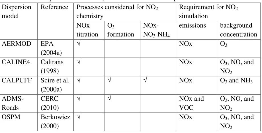
The chemistry module in dispersion models has been used to simulate NO2
concentration. The chemistry module in the five above-mentioned dispersion models was
compared in Table 2.2.
Table 2.2: A comparison of chemistry modules used in five dispersion models Dispersion
model
Reference Processes considered for NO2
chemistry
Requirement for NO2
simulation NOx titration O3 formation NOx- NO3-NH4
emissions background
concentration
AERMOD EPA
(2004a)
√ NOx O3
CALINE4 Caltrans
(1998)
√ NOx O3, NO, and
NO2
CALPUFF Scire et al. (2000a)
√ √ √ NOx O3 and NH3
ADMS-Roads
CERC (2010)
√ √ NOx and
VOC
O3, NO, and
NO2
OSPM Berkowicz
(2000)
√ NOx O3, NO, and
NO2
Because a majority of NO2 is formed by secondary chemical reactions in the
(Reaction 2.4). However, requirements for NO2 simulation differ among these three
models. The AERMOD only needs the background concentrations of O3 whereas
CALINE4 and OPSM need background concentrations of O3, NO, and NO2. This
difference in input requirements is due to the assumptions used by each model to
represent the NOx titration. The ADMS-Roads considers both NOx titration and O3
formation processes. It requires both NOx and VOC emissions. The CALPUFF considers
the NOx-NO3-NH4 process in addition to NOx titration and O3 formation processes. This
is because it is used to estimate long-range transport of pollutants.
2.2Vehicular emission models
Generally, vehicular emissions are estimated using collected or estimated traffic counts
along with emission factors of vehicles: the amount of emission emitted from each
vehicle per distance traveled (mass/vehicle/distance). Emission factors of vehicles are
determined based on vehicle types (e.g. light-duty, or heavy-duty), fuel types (e.g.
gasoline, or diesel), vehicle ages, and vehicle activities (e.g. cold start, or running), traffic
conditions (e.g. speed, acceleration, driving cycle), ambient conditions (e.g. temperature
and humidity), etc. Based on the above factors, emission factors of vehicles are
determined by testing vehicles on the dynamometers under different conditions.
Two types of models have been used for estimating emission factors of vehicles: first,
macroscopic models which calculate emission factors of vehicles based on average speed
of vehicles using different driving cycles, e.g. Mobile6.2; and second, microscopic
emission factor models which calculate emission factors based on instantaneous speed
For the estimation of emission factors, five models were evaluated: Mobile6.2 (EPA,
2003), Mobile6.2C (Vitale et al., 2004), MOVES (EPA, 2009), CMEM (University of
California, 2003) and backward spatial allocation of county-wide emission inventory
(Wang et al., 2009). These methods are compared in Table 2.3 with their advantages and
disadvantages.
Table 2.3: A comparison of evaluated methods for estimating emission factors Emission factor
model
Advantages Disadvantages
Mobile6.2 • Incorporate local fuel properties,
vehicle registration and ambient temperature
• User friendly
• Times consuming for running
and creating input/output files
Mobile6.2C • It is developed for Canada • No online version was available
MOVES • Similar to Mobile6.2,
incorporate local data
• Relational database
• Modal emission factors
• Sophisticated as it uses more
assumptions
CMEM • Consider emissions induced by
acceleration of vehicles,
particularly, heavy-duty trucks
• Trucks emission factors for
model year after 2001 is not available
• Instantaneous speed and
acceleration are not readily available
Spatial allocation of county-wide emission inventory
• High spatial coverage • Required city-wide vehicle
counts
• Not suitable for a road
Mobile6.2 released in 2003 is the EPA highway emission estimation model (EPA,
2003). It incorporates local fuel properties, vehicle age distributions, and ambient
(Moblie6.2C). Although Mobile6.2C was developed for Canada (Vitale et al., 2004), it
might be deemed not suitable for all places in Canada as vehicle age distribution and fuel
properties are different by province.
The MOVES is the most recent EPA mobile source emission model. MOVES
replaced the Mobile6.2 for regulatory purposes in 2010. In comparison to Mobile6.2,
MOVES is more comprehensive as it uses relational database and is able to estimate
modal emissions, emissions from alternative fuels and vehicles, GHG emissions, and fuel
consumption. In comparison to Moblie6.2, MOVES uses more extensive sets of default
input values. This may result in uncertainty in estimation of emissions, where local data
are not available or costly to collect.
The Comprehensive Modal Emission Model (CMEM) was developed by the
University of California in 2003. The CMEM can simulate instantaneous vehicular
emission using instantaneous speed and acceleration of vehicles. The model can estimate
emissions induced by acceleration and idling of vehicles. It has been observed that
emission rates of vehicles are higher when they accelerate compared to when they cruise
(Panis et al., 2006; Chen. et al., 2007). Acceleration and idling of vehicles are more
frequent at arterial roads, where vehicles stop and go due to facing signalized
intersections. Many studies used traffic simulation and CMEM to estimate vehicular
emissions (Kun and Lie, 2007; Boriboonsomsin and Barth, 2008). However, data
processing, calibration and validation of traffic simulation models are time consuming
and burdensome.
Wang et al. (2009) developed a method to allocate county-wide total mobile source
This allocation was carried out using some relevant surrogates such as roadway mile
traveled. Then, the census track benzene emissions are allocated to roadways using
vehicle counts as a surrogate. The backward spatial allocation of county-wide emission
inventory requires city-wide vehicle counts for road network which may not be readily
available.
An overview of emission and dispersion models used for traffic-related air quality can
be found in Fu and Yun (2010). Pierce et al. (2008) also conducted a comprehensive
review of these models, and it is suggested for further information.
2.3Selection of dispersion and emission models
The AERMOD dispersion model was selected. This is because it is the most advanced
dispersion model by EPA, and it needs the minimum requirements for NO2 simulation. It
has been used for estimation of NO2 (Chaix et al., 2006; Lindgren et al., 2009; Lindgren
et al., 2010) and benzene (Touma et al., 2007; Cook et al., 2008; Venkatram et al., 2009;
Wang et al., 2009) concentrations in several studies. For instance, Touma et al. (2007)
modeled benzene concentrations from several sources including roadways. Cook et al.
(2008) and Venkatram et al. (2009) estimated the benzene concentrations near roadways.
Wang et al. (2009) estimated benzene concentrations in Camden, New Jersey, and then
estimated personal exposure to this pollutant.
Among emission models, Mobile6.2 was selected. It has been most widely used for
estimating emissions in different studies. For instance, Cook et al. (2008) used Mobil6.2
to generate a look-up table for the calendar year 2002. The table provides emission factor
for estimation of vehicular emissions and dispersion of air pollutants (Cook et al., 2008;
Venkatram et al., 2009).
Mobile6.2 and AERMOD were used in many studies to estimate emissions and
concentrations (Sosa et al., 2012; Cook et al., 2008). Sosa et al. (2012) used Mobile6.2
and AERMOD to estimate air pollutant concentrations from border crossing traffic on the
Bridge of Americas, a major US-Mexico border. They evaluated effects of different
mitigation scenarios, and found that shifting commercial vehicles to other border crossing
and replacing them with passenger cars decreased the future level of NOx and PM2.5
concentrations. Hourly vehicle counts were collected for one-week in each of four
seasons (spring, summer, fall, and winter), and then hour-of-day emissions by season
were estimated. In another study, Cook et al. (2008) used Mobile6.2 and AERMOD to
estimate concentrations from traffic on roadways. They also considered emissions from
major industrial sources and household activities.
2.4Relationship between NO2 and benzene concentrations
NO2 and benzene are known to be traffic markers in urban air pollution. NO2 is mainly
from diesel vehicles whereas benzene is from gasoline vehicles. NO2 contributes to
formation of photochemical smog and ground-level O3 through complex chemical and
photochemical reactions with NO, O3, and VOCs. Acute short-term exposure to NO2 may
lead to change in airway responsiveness and lung function (EPA, 2012c). Long-term
exposure may lead to chronic bronchitis, and other respiratory infections. Similar to NO2,
the primary source of benzene emission is traffic. Vehicular benzene emissions are from
some aromatic compounds, and 3) evaporative losses. Short-term exposure to benzene
may cause drowsiness and headaches, and long-term exposure may cause cancer (EPA,
2012d).
The major source of NO2 and benzene in urban areas is traffic. Therefore, it is
expected that ambient concentrations of these two pollutants are positively correlated. In
this regard, several experimental studies have investigated the correlation between
ambient air concentrations of benzene and NO2 near the roadways (Modig et al., 2004;
Schnitzhofer et al., 2008; Beckerman et al., 2008) or in urban areas (Wheeler et al., 2008;
Parra et al., 2009). Some of these studies found a significant correlation between ambient
air concentrations of NO2 and benzene. This suggests that NO2 can be used as an
indicator of ambient benzene concentrations (Wheeler et al., 2008; Modig et al., 2004).
Kourtidis et al. (2002) measured ambient air concentration of NO2, benzene, and
some other pollutants in a street canyon. A strong correlation was observed between NO2
and benzene due to the fact that both were from traffic. Modig et al. (2004) conducted a
study to investigate whether “NO2 could be used to indicate ambient and personal levels
of benzene”. In this regard, personal levels of NO2 and benzene were measured for 40
participants for one week. The authors simultaneously collected ambient NO2 and
benzene concentrations at “one urban background station and one street station in the
city”. Results showed an insignificant correlation between personal levels of NO2 and
benzene (r=0.1, p=0.46). However, a strong correlation between ambient levels of NO2
and benzene was observed at both stations (r=0.7, p<0.05). Beckerman et al. (2008)
collected ambient concentrations of NO2, benzene, and some other air pollutants at two
Authors found a strong correlation between NO2 and benzene concentrations at receptors
located at one transect, MOE Station, (r = 0.94, p < 0.01), and no correlation at receptors
located at the other transect, the Bayview Station (r = 0.12, p > 0.05). The correlation was
not significant at the Bayview Station because it was located at a hilly area, and there
were some emission sources other than the Expressway such as “a major commercial
center and busy arterial road”. They concluded that “urban landscape, traffic patterns,
local topography, atmospheric chemistry and physical processes all appear to influence
the correlations between NO2 and other pollutants” (Beckerman et al., 2008).
Wheeler et al. (2008) collected ambient levels of NO2, benzene and some other
pollutants at 54 locations across Windsor, Ontario over four seasons of the year. They
observed significant correlations between NO2 and benzene concentrations (r = 0.89, p <
0.01). Parra et al. (2009) measured ambient air concentrations of VOCs and NO2 at 40
locations of Pamplona in Navarra, Spain. They found a strong correlation between the
NO2 and benzene concentrations (r = 0.59, p < 0.01), and suggested that NO2 can be used
as an indicator of benzene concentrations.
Schnitzhofer et al. (2008) measured “CO, NO, NO2, benzene, toluene and PM10 at a
motorway location in an Austrian valley” for one year. The authors found strong
correlations between heavy-duty vehicle counts and NO2 concentrations, and between
light-duty vehicle counts and CO concentrations. They also observed a strong correlation
between CO and benzene. This is because the primary source of these two pollutants is
light-duty vehicles. However, the authors did not report the correlation between NO2 and
Table 2.4 lists observed ratios of NO2/benzene concentrations in some of previous
studies. Two distinct groups of ratios were 37-39 and 25-26. Because both NO2 and
benzene are mainly from traffic, the ratio of NO2/benzene concentrations should be
similar to the ratio of NOx/benzene emissions. Using default values of Mobile6.2 and the
average speed of 60km/h, the NOx/benzene emission ratios were approximately 27 and
700 for passenger cars and heavy duty trucks, respectively. The observed ratio of 25-26
by Modig et al. (2008) and Wheeler et al. (2008) is close to the NOx/benzene emission
ratio for passenger cars. This reflects that the major traffic affecting NO2/benzene
concentration ratio was car traffic in these two studies. On the other hand, the observed
ratio of 37-39 by Schnitzhofer et al. (2008) and Beckerman et al. (2008) is higher than the
NOx/benzene emission ratios of passenger cars.
Table 2.4: Observed NO2/benzene ratios in previous studies
Study Source type Location NO2 (ug/m3) Benzene
(ug/m3)
NO2/Benzene
Modig et al. (2004)
Street station Sweden 53.0 2.1 25.2 Urban background Sweden 26.0 1.0 26.0 Schnitzhofer
et al., (2008)
Near road Austria 72.0 1.9* 37.9
Beckerman et al., (2008)
Near expressway Canada, Toronto
27.4* 0.7 39.2
Near expressway (Hilly area)
Canada, Toronto
32.9* 0.9 36.6
Wheeler et al., (2008)
Across urban area Canada, Windsor
23.3* 0.9 25.9
* Converted from ppb to µg/m3, assuming 1 ppb (NO2)=1.88 µg/m3(NO2), 1 ppb (Benzene)=3.19
µg/m3(Benzene) under standard condition
The cause of the correlation between NO2 and benzene concentrations in urban areas
can affect the correlation between NO2 and benzene concentrations as diesel vehicles are
high NOx emitters and gasoline vehicles are high benzene emitters. For example, the
NOx emission factor of heavy duty trucks is 16 times that of passenger cars (Transport
Canada, 2006). On the other hand, the benzene emission factor of passenger cars is four
times that of heavy duty trucks (Claggett & Houk, 2007).
2.5Limitations in the current literature
2.5.1 Vehicle counts
Accurate estimation of vehicular emission inventory and concentrations relies on accurate
estimation of traffic counts. Given that vehicle counts change over time, short-term data
collection does not take into account the day-to-day variation in peak-hour volume
(Hellinga and Abdy, 2008). To account for the variations in vehicle counts over time,
vehicle counts should be collected at various locations for a longer time period. The U.S.
Federal Highway Administration (FHWA) (2004) suggested that traffic counts over
several days should be adjusted to a typical day using adjustment factors. In this regard,
Kim (2003) adjusted vehicle counts collected in different survey times using the annual
average daily traffic (AADT) at each intersection.
In particular, the use of short-term data for the estimation of volume and traffic delay
may result in a large uncertainty. Some studies addressed this problem by collecting
long-term traffic counts. Capparuccini et al. (2008) evaluated the accuracy of design hourly
volume (DHV) estimated using short-term traffic counts. They collected hourly traffic
counts for a year and found that DHV obtained based on short-term traffic counts was