It is well known that cycle times in capacitated production systems increase nonlinearly with
resource utilization, which creates considerable difficulty for the traditional linear
programming (LP) models used for production planning. Clearing Functions capture this nonlinear relationship and embed it in the optimization model. In this thesis, we evaluate the
fitting methodology for clearing functions and show the importance of the fitting
methodology on the production planning. We then perform a systematic comparison of the
production planning models incorporating the clearing functions with the conventional linear
programming models for production planning under different scenarios. The computational
experiments applied to a scaled-down semiconductor manufacturing line illustrate the
by
Durmus Fatih Irdem
A thesis submitted to the Graduate Faculty of North Carolina State University
in partial fulfillment of the requirements for the degree of
Master of Science
Industrial Engineering
Raleigh, North Carolina
2009
APPROVED BY:
_______________________________ ______________________________
Dr. Reha Uzsoy Dr. Thom J. Hodgson
Committee Chair
DEDICATION
This thesis is dedicated to My Parents,
BIOGRAPHY
D. Fatih İrdem was born in Manisa, Turkey on July 3rd, 1984. He received his Bachelor of Science degree in Engineering Management from Istanbul Technical University,
Turkey. He joined North Carolina State University to pursue his Master of Science degree in
Industrial Engineering, in August 2007. During his graduate studies in the Edward P. Fitts
Department of Industrial Engineering, he worked as research assistant for Dr. Reha Uzsoy.
He has accepted a full time position with Schneider Electric in Lexington, KY, where he will
ACKNOWLEDGEMENTS
I would like to express my appreciation and thanks to Dr. Reha Uzsoy, my advisor,
for the initiation of my research and for his constant support and guidance during my studies.
I am very grateful for providing me the opportunity of pursuing my graduate studies at North
Carolina State University and working so closely with him. I would also like to thank to the
other members of my thesis committee: Dr. Thom J. Hodgson and Dr. Brian Denton for
serving on the committee, expressing interest in and reviewing my thesis.
I have also been incredibly fortunate to have made very good friends (you all know
who you are!) during my life in Raleigh, NCand I extend my sincere gratitude to you all for
your help, friendship, understanding and patience.
I am also thankful to my family in Turkey for their unconditional suppo rt, love and
trust throughout my life. To my fiancée Güler: thank you for your never ending love,
precious support and continuous motivation for six years. Words are not enough to express
TABLE OF CONTENTS
LIST OF TABLES ... vii
LIST OF FIGURES ... viii
1 INTRODUCTION ... 1
2 PREVIOUS RELATED WORK ... 5
2.1 MATERIAL REQUIREMENTS PLANNING (MRP) ... 6
2.2 LINEAR PROGRAMMING MODELS ... 7
2.3 ITERATIVE PROCEDURES ... 8
2.4 MODELS INCORPORATING LOAD DEPENDENT LEAD TIMES ... 9
3 COMPARISON OF ALGORITHMS ... 13
3.1 HUNG AND LEACHMAN (HL)PROCEDURE... 13
3.1.1 The Linear Programming Model ... 14
3.1.2 The Iterative Procedure ... 18
3.2 ALLOCATED CLEARING FUNCTION (ACF)MODEL ... 19
3.2.1 The Linear Programming Model ... 20
4 EXPERIMENTAL DESIGN ... 23
4.1 THE SIMULATION MODEL... 23
4.2 EXPERIMENTAL FACTORS... 27
4.3 THE LPENVIRONMENT ... 29
4.3.1 Capacity Adjustment in the HL Model ... 30
4.4 GENERATION OF CLEARING FUNCTIONS ... 32
4.4.1 Generation of WIP-Output Data from Simulation ... 33
4.4.2 Comparisons of Different Clearing Function Data Sets ... 39
4.4.3 Clearing Function Fitting Methodology ... 43
4.4.4 Piecewise Linearization ... 50
5 EXPERIMENTAL RESULTS ... 57
5.1 CASE 1–(SHORT,70%,CONSTANT) ... 58
5.2 CASE 2–(SHORT,70%,VARYING) ... 61
5.3 CASE 3–(SHORT,90%,CONSTANT) ... 64
5.4 CASE 4–(SHORT,90%,VARYING) ... 67
5.5 CASE 5–(LONG,70%,CONSTANT) ... 69
5.6 CASE 6–(LONG,70%,VARYING)... 72
5.7 CASE 7–(LONG,90%,CONSTANT) ... 74
5.8 CASE 8–(LONG,90%,VARYING)... 76
5.9 SUMMARY ... 79
6 CONCLUSIONS... 80
6.1 CONCLUSIONS ... 80
6.2 FUTURE DIRECTIONS... 82
LIST OF TABLES
Table 4.1 Breakdown distribution parameters for short failure case ... 24
Table 4.2 Breakdown distribution parameters for long failure case ... 24
Table 4.3 Simulation processing times and batch sizes ... 25
Table 5.1 Experimental Scenarios ... 58
Table 5.2 Standard deviation values for case 1... 61
Table 5.3 Standard deviation values for case 2... 64
Table 5.4 Standard deviation values for case 3... 66
Table 5.5 Standard deviation values for case 4... 68
Table 5.6 Standard deviation values for case 5... 71
Table 5.7 Standard deviation values for case 6... 73
Table 5.8 Standard deviation values for case 7... 76
LIST OF FIGURES
Figure 1.1 Relationship between lead time and utilization ...2
Figure 2.1 Different forms of clearing functions ...9
Figure 3.1 Flow conservation ... 22
Figure 4.1 Schematic of wafer fabrication line ... 26
Figure 4.2 Varying demand pattern for 90% utilization... 29
Figure 4.3 Varying demand pattern for 70% utilization... 29
Figure 4.4 Generation of clearing function data ... 36
Figure 4.5 [WIP,X] data for station 1 ... 37
Figure 4.6 [WIP,X] data for station 3 ... 38
Figure 4.7 [WIP,X] data for station 7 ... 38
Figure 4.8 [WIP,X] data for station 4 ... 39
Figure 4.9 Clearing function slopes for station 1 ... 41
Figure 4.10 Clearing function slopes for station 3 ... 41
Figure 4.11 Clearing function slopes for station 7 ... 42
Figure 4.12 Clearing function slopes for station 4 ... 42
Figure 4.13 Fitted F1 for station 1 ... 44
Figure 4.14 Fitted F1 for station 3 ... 45
Figure 4.15 Fitted F1 for station 7 ... 45
Figure 4.17 Fitted F2 for station 1 ... 47
Figure 4.18 Fitted F2 for station 3 ... 48
Figure 4.19 Fitted F2 for station 7 ... 48
Figure 4.20 Fitted F2 for station 4 ... 49
Figure 4.21 Linearization of the clearing function... 51
Figure 4.22 Complementary lines used in linearization ... 52
Figure 4.23 Minimization of the area between lines and curve ... 54
Figure 4.24 Clearing function with F1 for station 4 ... 55
Figure 4.25 Clearing function with F2 for station 4 ... 56
Figure 5.1 Case 1, HL model, planned vs. realized outputs ... 59
Figure 5.2 Case 1, ACF model, planned vs. realized outputs ... 60
Figure 5.3 Case 2, HL model, planned vs. realized outputs ... 62
Figure 5.4 Case 2, ACF model, planned vs. realized outputs ... 63
Figure 5.5 Case 3, HL model, planned vs. realized outputs ... 65
Figure 5.6 Case 3, ACF model, planned vs. realized outputs ... 66
Figure 5.7 Case 4, HL model, planned vs. realized outputs ... 67
Figure 5.8 Case 4, ACF model, planned vs. realized outputs ... 68
Figure 5.9 Case 5, HL model, planned vs. realized outputs ... 70
Figure 5.10 Case 5, ACF model, planned vs. realized outputs ... 71
Figure 5.11 Case 6, HL model, planned vs. realized outputs ... 72
Figure 5.13 Case 7, HL model, planned vs. realized outputs ... 74
Figure 5.14 Case 7, ACF model, planned vs. realized outputs ... 75
Figure 5.15 Case 8, HL model, planned vs. realized outputs ... 77
CHAPTER 1
1
INTRODUCTION
Meeting customer demands on time is an important issue in today’s competitive
business environment, and has motivated extensive interest and investment in production
planning systems. Production planning can be defined as the determination of future
production and inventory quantities. An important decision here is the timing of the releases
so that the output meets market demand on time. In order to do that, we have to know the
lead time of production facility, which is the time between release of work and its emergence
as finished product. The importance of production planning has motivated researchers and
practitioners to improve production planning methodology and practices over the last fifty
years. The production planning methods commonly used in industry include the Materials
Requirements Planning (MRP) discussed by Orlicky [1] and a variety of linear programming
models such as those described by Woodruff and Voss [2], Johnson and Montgomery [3] and
MRP [1] uses a backward scheduling logic for the production releases. The
production requirements are offset from delivery dates using constant lead time parameters.
The algorithm treats the lead times as exogenous parameters that do not depend on the
utilization level or the capacity of the system. However, queuing models [5, 6] have shown
that average cycle times will depend on the resource utilization, i.e. there is a highly
nonlinear relationship between the cycle times and resource utilization as reflected in Figure
1.1.
Figure 1.1 Relationship between lead time and utilization
This relationship leads to a circularity problem for traditional production planning
methods such as MRP and linear programming. In order to release work into the plant to
complete on time to meet demand, the algorithm must have some knowledge of lead times.
However, the material release decisions obtained from the planning algorithm affect the
resource utilizations, which in turn results in changes in lead times. MRP does not consider
the effect of capacity loading on work in process and lead times. Conventional linear
100%
programming models take resource capacity constraints into account to ensure that the
production plans are capacity feasible at an aggregate level and the customer demands are
met on time by using fixed lead time estimates. However, similar to MRP, they do not
consider the relationship between cycle time and resource utilization. This circularity has
been present in most production planning research since the initial work in the field in the
1950s, and is seldom addressed in the literature.
In recent years there have been a growing number of research efforts to develop
computationally tractable production planning models that address this circularity [7, 8]. In
this thesis we focus on a promising technique that has emerged recently, that of models based
on clearing functions. The basic idea of the clearing function is to define the expected
throughput of a resource over a given period as a function of average work in process
inventory (WIP) over that period. Different forms of clearing functions have been proposed
in [9, 10, 11]. Clearing function approach does not require any exogenous lead time
parameter inputs, since the clearing function models them implicitly. It has been found that at
least under some conditions, the clearing function approach represents the capabilities of
manufacturing systems more accurately than the conventional linear programming models [7,
8]. However, there are a number of open questions regarding the best way to estimate the
clearing functions representing production resources such as machines. In order to address
these questions, in this thesis we combine a variety of clearing function ideas and analyze
clearing functions have a strong dependence on the production planning procedure used to
estimate them, which would introduce a new circularity if it were to hold.
Thus, the objectives of our research can be stated as follows:
• To test the performance of production planning models using different functional
forms of clearing functions under different operating conditions. The performance of
the different models will be compared to conventional LP models as well as iterative
algorithms combining LP models and simulation, using a simulation model of a
scaled-down wafer fabrication facility as a testbed.
• To examine whether the form of clearing functions are static or dynamic.
• To develop an automated computational infrastructure that performs all the tasks to fit
the clearing function.
The thesis is composed of five chapters in addition to this chapter. The chapters are
organized as follows. In Chapter 2, we present a brief review of previous research related to
our thesis. In Chapter 3 we explain the algorithms that we use and compare in our
experiments, in detail. In Chapter 4, we present the experimental design that consists of our
simulation model of the wafer fab, the LP environment and how we generate the clearing
functions. The purpose of this chapter is to give the insights to the reader about the process of
implementing the ACF model. In Chapter 5, we present and interpret our experimental
results. We conclude the thesis with a summary of the results obtained and point out the
CHAPTER 2
2
PREVIOUS RELATED WORK
As discussed in the previous chapter, the fundamental circularity problem has been
studied in production planning research area since the 1950’s [12]. There have been three
main approaches in the literature that address this problem. The first group includes methods
that assume the lead times are exogenous parameters that are independent of resource
utilization. This category consists of the MRP [1] and most Linear Programming Models [4].
The second approach includes the of use either a detailed scheduling algorithm [13] or a
simulation model for verifying the feasibility of the production planning model [14, 15]. This
approach is good at capturing the queuing behavior of the production resources; however it
does not scale well to large and complex systems due to the computational time and data
requirements. This second approach has formed the basis for iterative methods that combine
linear programming and simulation models. The procedure by Hung and Leachman [14] is
the best known of these methods. The third approach has been to model the nonlinear
dynamics directly, using models incorporating load-dependent lead times. These approaches
inventories (WIP) to the objective function [16], and optimization models with constraints
based on clearing functions, the main topic of this thesis, which relate the expected WIP level
in a planning period to the expected output [9, 10, 11, 17, 18].
2.1 Material Requirements Planning (MRP)
MRP, which has been the basis for the most management information systems that
support production planning and control in industry, is described by Orlicky [1]. One of the
major weaknesses of MRP is that lead times are treated as resource independent parameters
in the algorithm. However, lead times are always a result of planning and cannot be defines
as given parameters. Moreover, the MRP method is unable to handle the resource capacities,
which may result in infeasible production plans.
The MRP concept has given rise to a variety of extensions that aim to overcome its
weaknesses. In order to address this, the Capacitated Material Requirements Planning
(MRP-C) was developed by Tardif and Spearman [19], which extends MRP to consider limited
capacity, and provide feedback in case of an infeasible production plan so the user can
change the production plan to achieve feasibility by adding capacity.
However, the MRP-C procedure has some drawbacks when multiple products are
considered. When a resource is used by multiple products, the capacity allocation among
2.2 Linear Programming Models
Typical goals of a production planning process are to meet the customer demands on
time and maximize the profit or minimize the costs while doing so. Linear programming is
one of the most traditional approaches to formulate this problem. Given a set of variables, the
linear programming model works by maximizing or minimizing a linear objective function
over a set of constraints. In conventional LP models, these constraints are generally on
resource capacities, inventory balance and material flows.
The constraints representing the resource capacities have usually a fixed right-hand
side value which represents an upper bound on the capacity available in a given time period
as follows:
∑
∀
≤
i it it t
C X
α , (2.1)
where αit denotes the unit capacity consumption rate of product i in period t, Xit the amount of
product i produced in period t and Ct the available capacity of the corresponding resource in
period t. In addition to constraints on resource capacities, another common constraint characterizes the inventory balance and the fulfillment of customer demand. The most
common way to apply this constraint is as follows:
it it it
it I R D
I = −1 + − , (2.2)
where Iit denotes the amount of finished goods inventory from product i at the end of period
t, Rit the amount of released material of product i into the plant in period t and Dit the
The problem with this kind of model is that the production occurs instantaneously as
the materials are released into the system, because these models assume that lead times are
less than one period. In order to handle the instantaneous production problem, Hax and
Candea [20] have proposed a linear programming model with integer time lags which
provides a relationship between the releases and output with a given lead time as follows:
L it it X
R = + , (2.3)
where L denotes the integer lead time for product i. The equation states that the released material in period t emerges as finished product in period t+L. The problem with integer lead times is that it may give an optimal solution which may be physically infeasible. Hackman
and Leachman [4] have extended this approach to a model with non-integer lead times.
However, as in MRP, none of these models can capture the nonlinear relationship between
lead times and utilization.
2.3 Iterative Procedures
As we discussed in the previous chapter, the lead times are determined by resource
utilization which is determined by the release plan, representing the planning circularity. In
the linear programming models explained above, the lead times used to model the
input-output relationship are treated as constant but will actually change depending on the starts. In
order to address the circularity problem, Hung and Leachman [14] have proposed an iterative
procedure which iterates between an LP model, which takes the lead times as input from the
from LP model. The hope is that this will converge to an optimal, although convergence is
not guaranteed. This method has a number of advantages, but does not appear to have been
tested over a range of different operating conditions due to the highly time consuming nature
of experiments. More importantly, it is questionable if this approach converges to a global
optimal solution, or in fact whether it will consistently converge.
2.4 Models Incorporating Load Dependent Lead Times
The question of how to develop a production planning model which captures the
nonlinear relationship between lead times and workload has motivated the clearing function
approach which models this relationship directly in the optimization model. Figure 2.1
illustrates some possible forms of clearing functions studied by the researchers to date.
Figure 2.1 Different forms of clearing functions Nonlinear
(Srinivasan, Karmarkar)
Combined Fixed Capacity (LP)
Constant Proportion (Graves)
Output
Graves [9] opens the discussion of clearing functions by defining a linear function
with clearing factor α, which represents the fraction of WIP that is processed in the given
period. The linear clearing function of Graves [9] is as follows:
WIP Throughput
Expected =α× (2.4)
Like MRP, this form of clearing function does not take finite resource capacities into
account; by applying Little’s Law, it is clear that the model maintains a fixed lead time even
when the machine loads change. It may also lead to infeasible solutions at high utilization
levels. This idea was extended to a nonlinear clearing function in [10, 11], which considers
finite capacity. In the nonlinear clearing function, it is assumed that throughput of the period
is a concave nondecreasing function of the average WIP level over that period. They
incorporate the clearing function into an optimization model by relating the average WIP
levels to an expected output level.
Srinivasan et al. [10] and Karmarkar [11] suggest two different functional forms for
the clearing function that can be fit to empirical data or data from a simulation model.
Srinivasan et al. [10] propose a concave exponential function of the form
0 ) 0 ( ) 1 ( ) ( 2
1 − =
=K e− f
W
f KW
(2.5) while Karmarkar [11] suggests the alternative form
In both of these forms, K1 and K2 are the parameters determined for fitting the functions to
the empirical data. K1 represents the maximum possible output, while K2 determines the
curvature of the clearing function.
The nonlinear clearing function is extended to an allocated clearing function form in
[18], which utilizes a partitioning scheme for applying the concept to multi-product
environments. The difficulty in the multi-product situation is that the products compete for
capacity at a given resource, which may cause a situation where the WIP of one product type
is delayed in the system in order to process other products with shorter lead times. The
partitioned clearing function addresses this problem by decomposing the overall clearing
function into a set of functions that represent the allocation of the expected output among the
products.
As seen in Figure 2.1, the constant proportion clearing function, proposed by Graves
[9], does not have any restriction on the level of output. The fixed capacity function
corresponds to a fixed upper bound for capacity as used in most conventional linear
programming models. However, this type of function does not consider the lead time
constraints, which results in instantaneous production. The combined form of clearing
functions represents a combination the fixed capacity and constant proportion functions.
Combined clearing function imposes an upper bound for the capacity in case of the WIP
level exceeds a point. The combined clearing functions underestimate the expected output in
Having explained the methods developed in production planning area since 1950’s,
we now have an idea of fundamental problems in this area and developed approaches to
solve these problems. In the next chapter, we will shed light on the algorithms that we will
use in our experiments. We will first start with a fixed lead time model, i.e. Hung and
Leachman (HL) procedure [14] and then give the details of the clearing function model, i.e.
CHAPTER 3
3
COMPARISON OF ALGORITHMS
In this chapter, we introduce the production planning algorithms that we compare in
our experiments. The first of these, the Hung and Leachman (HL) procedure [14], is an
iterative procedure which combines optimization and simulation. This is an example of a
fixed lead time model used in an iterative scheme with a simulation model. We compare this
iterative algorithm with an algorithm that utilizes clearing functions, which we will refer to
as the Allocated Clearing Function (ACF) Model [18]. It should be noted that the ACF model
uses a separate clearing function for each workstation in the system. The difference between
these two algorithms is that the HL procedure (fixed lead time model) uses the lead time
estimates obtained from simulation, while the ACF model takes the clearing functions as
input and determines the lead times dynamically.
3.1 Hung and Leachman (HL) Procedure
Hung and Leachman [14] have proposed an elegantly intuitive solution to production
LP model for production planning, which takes flow time estimates as inputs and determines
a profit-maximizing release pattern over the planning horizon; and a detailed simulation
model of the production facility, which takes as input the release pattern determined by the
LP model and returns estimates of the flow times that would be realized by the facility under
that release pattern. The new flow time estimates are then input into a new LP model, and the
procedure iterates until some convergence criterion is satisfied. They apply their approach to
an industrial data set, and report that the procedure converges according to their criteria.
3.1.1 The Linear Programming Model
The HL algorithm follows the conventional LP approach of dividing the planning
horizon, the time interval over which decisions are to be made, into discrete planning
periods. The production process for a product is represented as a series of operations; due to
the reentrant routings in wafer fabs, multiple operations may use the same equipment. The
model used is essentially the Step-Separated formulation of Leachman and Carmon (1992),
which requires the estimated lead times Fgl required for a lot of product g to reach operation l
after being released into the plant. However, instead of fixed lead times that remain constant
over the entire planning horizon, the authors associate values of the lead time parameters
with the start of each planning period. In the following p=0 is the start of period 1, p=1 is the start of period 2, etc., that is, a time unit is the period length. The lead time parameters Fgpl,
in the time interval Q = [(p-1)- Fg,p-1,l, p- Fgpl], assuming planning period p starts at time
(p-1). The crux of the formulation is relating the resource loading Ygp by product g in period p to
the amount of product g released over time. We shall use the following notation:
τg,p: number of working days for wafer type g from start of period 1 (time 0) until the end of
period p, p=1,2,…,P.
[τ]+: smallest index p such that τ g,p> τ.
Fg,p,l: the expected flow time from wafer release to operation l, occurring at epoch τg,p.
Fg,p: the expected flow time from wafer release to finish, occurring at epoch τg,p.
Ygpl: wafer quantity consuming machine hours at operation l for wafer type g in period p.
Ygp: wafer output quantity for wafer type g in period p.
Xgp: wafer release quantity for wafer type g in period p.
[
]
+ − − −= − l p g p g Fp τ , 1 , 1, (3.1)
[
]
+ + = − l p g p g Fp τ , , , (3.2)
There are two cases to consider here. In the first, simpler case, the time interval Q lies within a single planning period, and the amount Ygpl of product g loading resources at
operation l in period p is given by
+ + + − − − − − − − = gp p g p g l p g p g l p g p g gpl X F F Y ) ( ) ( ) ( 1 , , , 1 , 1 , , , , τ τ τ τ (3.3)
duration included in the interval Q (again assuming uniform release rates within the planning periods). This yields:
+ + + + + − − − − − − − − + − − − − − − + + − − −
=
∑
gpp g p g p g l p g p g p p gp gp p g p g l p g p g p g gpl X F X X F Y ) ( ) ( ) ( ) ( 1 , , 1 , , , , 1 1 1 , , , 1 , 1 , , τ τ τ τ τ τ τ τ (3.4)
The LP formulation maximizes profit subject to constraints on material flow and
resource capacities. An artificial final period with length equal to the longest flow time over
the horizon is added to ensure that an appropriate ending condition is achieved. We use the
following notation:
Decision Variables:
Xgp: Wafer release quantity for wafer type g in period p.
Igp: Units of product g in finished goods inventory at the end of period p.
Bgp: Units of product g backlogged at the end of period p.
Parameters:
aglk: Average machine hours of machine type k used in operation l of wafer type g.
Ckp: Hours of machine type k available in period p.
vgp: Unit revenue from product g in period p
cgp: Unit production cost of product g in period p.
hgp: Unit inventory holding cost for product g in period p.
bgp: Unit backlogging cost for product g in period p.
dgp: Demand for wafer type g in period p.
zpg: First frozen period of wafer type g. (The production rates after this period will be set
equal to the rate in this period in order to satisfy the steady-state horizon condition.)
spg: Earliest nonpositive period number in which current WIP would have started considering
the assumed flow times.
Xgp: Equivalent wafer releases generating the current WIP status of wafer type g, defined in
periods before the start of the planning horizon, p=0,-1,-2,…,- spg
gp
B : Upper bound on backlogs for wafer type g in period p.
The complete formulation is as follows:
∑∑
∑∑
∑∑
∑∑
∈ + = ∈ + = ∈ + = ∈ + = − − − G g Pp gp gp G
g P
p gp gp G
g P
p gp gp G
g P
p gp gp
B b I h X c Y v 1 1 1 1 1 1 1 1 max (3.5) Subject to: Resource Capacity: kp G g l l l gp glkY C
a g
≤
∑∑
∈ =1
p=1,…,P+1 for all k ∈ K (3.6)
Demand Equations:
∑
=
= +
− fpg
p gp gp
gp
gp I B d
Y
1
g ∈ G, p=fpg (3.7)
gp gp gp p g p g
gp I B I B d
Y + , −1− , −1− + = g ∈ G, p=fpg+1,…,P-1 (3.8)
gp gp p g
gp B B d
Variable Non-negativity:
0 ≥
gp
X g ∈ G, p=1,…,zpg (3.10)
0 ≥
gp
I g ∈ G, p=1,…,P-1 (3.11)
0 =
gp
I g ∈ G, p=P,P+1 (3.12)
gp gp B
B ≤ ≤
0 g ∈ G, p=1,…,P+1 (3.13)
3.1.2 The Iterative Procedure
Given the LP formulation above, the HL procedure performs the iterations between
LP and simulation model as follows:
Step 1: Set k = 1; MaxIT = 30; obtain initial flow time estimates 0 gpl
F . Set 0
gpl k
gpl =F
φ . In our
experiments the 0 gpl
F were obtained from a steady state simulation run with releases set equal
to period demand for each product.
Step 2: Solve the LP model using the flow time estimates k gpl
F to obtain the material release
schedule k
gp
X .
Step 3: Assuming the releases in each period are uniformly distributed over the period, use five independent replications of the simulation model to estimate the flow times k
gpl
F . The
mean of the sample values obtained from the simulation replications is used as the estimator.
lots thus generated (due to the difference between fractional and rounded values of the k gp
X )
are distributed evenly over the planning horizon to minimize their disruptive effects.
Step 4: If k < MaxIT, set k = k+1, = +(1− ) k−1 gpl k
gpl k
gpl αF α F
φ , where 0 ≤ α ≤ 1 is a u ser
-defined smoothing constant, and go to Step 2. Otherwise, stop.
The number of simulation replications was selected based on a tradeoff between the need to
obtain some statistical precision in our estimates of the flow times, while keeping the
computational burden of the overall iterative procedure within reasonable limits.
A more detailed discussion of HL procedure and detailed results obtained from application of
this procedure can be found in Irdem et al. [21].
3.2 Allocated Clearing Function (ACF) Model
The clearing function model that we use in this study is the Allocated Clearing
Function model developed by Asmundsson et al. [18]. This optimization model was
developed for a multistage multiproduct production system where each capacitated resource
is represented by constraints relating its expected throughput in a planning period to the
average WIP at that stage over that planning period. In addition to constraints representing
the relationship between output and WIP, the model also includes inventory balance
3.2.1 The Linear Programming Model
The linear programming model is formulated as a cost minimization problem. We
define the following notation for our LP model:
Decision variables:
n gp
R : Wafer release quantity for wafer type g at operation n during period p.
n gp
X : Wafer output quantity for wafer type g at operation n over period p.
gp
X : Production quantity for wafer type g over period p (Xgp=output of last operation).
n gp
W : WIP quantity for wafer type g at operation n over period p. This includes all jobs in
queue and being processed.
gp
I : Units of product g in finished goods inventory at the end of period p.
gp
B : Units of product g backlogged at the end of period p.
k gp
Z : The fraction of capacity at resource k and period p that is utilized by product g.
Parameters:
cgp: Unit production cost of product g in period p.
hgp: Unit inventory holding cost for product g in period p.
bgp: Unit backlogging cost for product g in period p.
wgp: Unit WIP holding cost for product g in period p.
dgp: Demand for wafer type g in period p.
c k
c k
β : Intercept of the linearized clearing function at segment c for resource k.
The complete formulation is as follows:
∑∑
∑∑
∑∑
∑∑
∈ = ∈ = ∈ = ∈ = + + + G g Pp gp gp G
g P
p gp gp G
g P
p gp gp G
g P
p gp gp
W w B b I h X c 1 1 1 1
min (3.14)
Subject to: WIP Flow: n gp n gp n p g n
gp W X R
W = , −1− + ∀p,g,n (3.15)
Inventory Balance: gp gp gp p g p g
gp I B I B d
X + , −1− , −1− + = ∀p,g (3.16)
Clearing Function (Output~WIP):
∑
∈ − + + ≤ K n k gp c k n p g n gp c k ngp W W Z
X α ( ) β
2 1
1
, ∀p,g,k,c (3.17)
Variable Non-negativity:
0
≥
gp
X ∀p,g (3.18)
0
≥
gp
R ∀p,g (3.19)
0
≥
gp
W ∀p,g (3.20)
0
≥
gp
I ∀p,g (3.21)
0
≥
gp
WIP (3.15) and inventory balance (3.16) constraints implement the flow conservation
which is also illustrated below in Figure 3.1.
Figure 3.1 Flow conservation
In this formulation, the decision variable n gp
W accounts for the WIP levels at the end
of period p. However, the WIP parameters which we obtain from simulation, in order to form
the clearing function, account for the average WIP levels over the corresponding period. Our
approach to this problem is to average the n gp
W variables for two consecutive periods, i.e.
) 1 , (
2
1 n
p g W n gp W
−
+ , which will give us an approximation of the average WIP level during the
period. The expected output for the corresponding period can be defined as a function of
average WIP by using this approximation.
FGI Releases
Inflow
Throughput Demand
CHAPTER 4
4
EXPERIMENTAL DESIGN
The objective of our experiments is to explore the behavior of the clearing function
models under a broad range of experimental conditions and to compare these results to the
performance of the HL algorithm. The two models explained in the previous chapter were
used to obtain production plans for a 26-week (semi-annual) planning horizon under the
different experimental conditions. Then, these plans were simulated to obtain the realized
plans and compare them with the suggested plans obtained from the optimization model. We
first describe the simulation model of the production system used as a testbed, then the
implementation of the optimization models, and finally present the design of our
experiments.
4.1 The Simulation Model
The production system was built based on the attributes of a real-world
semiconductor wafer fab environment [22]. The major characteristics of wafer fabrication,
multiple products with varying process routings are included in the model. The model was
built by defining a distinct re-entrant bottleneck representing the photolithography process.
The processing times for all other stations were scaled to the bottleneck processing time so
that no non-bottleneck station would have a utilization approaching that of the bottleneck.
The model has batching stations (Stations 1 and 2) early in the process, representing the
furnaces which perform the diffusion and oxidation processes. The minimum batch size
required is two lots and the maximum batch size is four lots. The batching stations can be
loaded with any product lot mix, that is, a batching station can run lots of one type of product
or many product types at one time. The remaining stations process one lot at a time. Table
4.1 and Table 4.2 show the distributions for the up and down time parameters for short
failure and long failure case, respectively.
Table 4.1 Breakdown distribution parameters for short failure case
Station # Alpha MTTF (in mins) Beta Alpha MTTR (in mins) Beta (Min/Max) Batch
3 7200 1 1200 1.5 2/4
7 7200 1 1200 1.5 2/4
(All MTTF and MTTR are Gamma Distributions)
Table 4.2 Breakdown distribution parameters for long failure case
Station # Alpha MTTF (in mins) Beta Alpha MTTR (in mins) Beta (Min/Max) Batch
3 14400 1 2400 1.5 2/4
7 14400 1 2400 1.5 2/4
The simulation model is made up of 11 stations, each with one server except the
bottleneck station (Station 4) that has two servers. The processing times for the stations are
lognormally distributed with the standard deviation less than or equal to 10 percent of the
mean. Table 4.3 shows the specific station processing times and batching sizes. The low
process variance is representative of automation and tight process specifications encountered
in the semiconductor industry.
Table 4.3 Simulation processing times and batch sizes
Station # Mean Std. Dev. Batch (Min/Max)
1 80 7 2/4
2 220 16 2/4
3 45 4 1
4 40 4 1
5 25 2 1
6 22 2.4 1
7 20 2 1
8 100 12 1
9 50 4 1
10 50 5 1
11 70 2.5 1
(All processing times are lognormal)
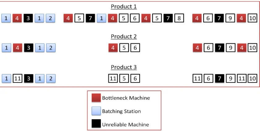
There are three products produced in the system with different complexity. Product 1
has 22 process steps including 6 visits to the bottleneck station. Product 2 has 14 process
steps with 4 visits to the bottleneck station. Product 3 has 14 process steps and does not visit
the bottleneck, but instead visits Station 11. The system is required to produce a product mix
in proportions of 3:1:1 of Product 1, 2, and 3 respectively. The workflow through the
Figure 4.1 Schematic of wafer fabrication line
Each row in the figure represents the routing of each product produced in the system.
The works flow from left to right, i.e. all products start the process at Station 1 and emerge as
a finished product after being processed in Station 10.
In the model, there are two unreliable stations that create most of the starvation at the
bottleneck. One station is visited only once by each product early in the process routings; for
simplicity, we shall refer to this station as the “Single Entry Machine”. The second
unreliable station is visited multiple times by the products and occurs later in the processing
steps. This station is representative of a Chemical Vapor Deposition (CVD) process that is
capable of producing a high output very quickly. This station will be referred to as the
“Multiple Entry Machine”. These two unreliable stations have the ability to produce a lot of
Lots are dispatched in First-in-First-Out order on all machines. The simulation model
was implemented in Arena Version 10.
the LP model using Excel and a number of Visual Basic scripts.
4.2 Experimental Factors
Our experiments were designed to examine the effects of three different factors on the
performance of the algorithms compared. These three factors are as follows:
A. Failure Pattern: We experiment with two different levels of machine failures to test the performance of algorithms under different system variabilities such as tolerable
failures and heavy failures. The numerical details of these two failure patterns are
given in Table 4.1 and Table 4.2
1) Short Failures: The machines subject to failures have mean time to failure values that are within a planning period. The machines are down more
frequently than the long failure factor, however, they are repaired quicker than
the long failure case.
2) Long Failures: The mean time to failure values are more than a period length. Basically, MTTF and MTTR values are twice as much as the values in short
failure case. Short failure and long failure cases both have the same machine
availability rates in average, however, the only difference is the frequency of
B. Bottleneck Utilization: It is well known from queuing theory that the nonlinear relationship between resource utilization and flow times becomes more severe at high
utilization levels. Hence one would expect an LP model using fixed lead time
estimates or clearing function to perform well at low utilization levels, but to degrade
in performance at higher utilization. Hence we experiment with two bottleneck
utilization values of 70% and 90%. The utilization level is achieved by varying the
demand of all products while maintaining the 3:1:1 product mix required by the
testbed, which means that the expected demand for Product 1 is three times the
expected demand levels for Product 2 and Product 3.
1) 70% Bottleneck Utilization 2) 90% Bottleneck Utilization C. Demand Profile:
1) Constant Demand: In order to test the algorithms under a favorable condition we keep the demand constant across the planning horizon of 26 weeks while
keeping the 3:1:1 product mix and yielding the targeted bottleneck utilization.
2) Varying Demand: We also use a varying demand profile in order to examine how the algorithms perform under a more complex demand scenario.
Similarly, we maintain the varying demand pattern, which is not random,
while satisfying the 3:1:1 product mix and targeted bottleneck utilizations.
Figure 4.2 Varying demand pattern for 90% utilization
Figure 4.3 Varying demand pattern for 70% utilization
4.3 The LP Environment
In our experiments, the LP models were implemented in the OPL Studio Version 5.5
modeling language by ILOG
0 15 30 45 60 75
0 10 20 30
D em and ( in uni ts ) Weeks
90% Bottleneck Utilization
Product 1 Product 2 Product 3 0 15 30 45 60 75
0 10 20 30
D em and ( in uni ts ) Weeks
70% Bottleneck Utilization
with a Intel(R) Core(TM) 2 CPU 6700 2.66 GHz processor and 2GB of RAM, under
Microsoft Windows XP Professional.
The models that we described in previous chapter were coded in OPL Studio and
supported by an Excel input file from which the optimization model reads the parameters.
4.3.1 Capacity Adjustment in the HL Model
As mentioned in section 4.1, our wafer fab has two unreliable stations which are
subject to failures. In order to represent the actual system capacity more accurately at the
optimization side, capacity adjustments were made to the right-hand side parameters of
capacity constraints. The resource capacity constraint of HL model was:
kp G g l l l gp glkY C
a g
≤
∑∑
∈ =1
for all k ∈ K, p ∈ P (4.1)
where Ckp denotes the available capacity at machine k during period p. The following
modification was made to this constraint for the experiments:
k kp G g l l l gp
glkY C Availability
a g * 1 ≤
∑∑
∈ = (4.2)where Availability = 0.8 for k=3 and k=7 (for unreliable stations) Availability = 1.0 for the other stations.
4.3.2 Transfer of LP Outputs to Simulation as Input
In order to obtain clearing function data from the simulation data or to perform
iteration between LP model and simulation model, we need to pass the release schedule data
simulation model. These release variables may be fractional, which have to be rounded to
integer values in order to be able to run the simulation model.
In addition to rounding release variables to integer values, we make an additional
change to release variables before inputting them to our simulation model. The production
planning LP model gives us release variables that represent the amount of materials released
into the system for each planning period, i.e. 1 week in the experiments. While releasing the
materials into the wafer fab in the simulation, we assume that the releases in a period are
uniformly distributed over the corresponding period. Thus, we divide the weekly release
amount by 7 and then round these daily release amounts to integer values to obtain integer
daily release amounts.
In order to apply the modifications mentioned above to release data, we use an
algorithm [23] that rounds some values up and some values down while matching the weekly
release amount in total. The algorithm starts by rounding the first value up and then checks
the difference between actual release amount and the rounded integer values. If the
cumulative difference is greater than 1, the next value is rounded down and otherwise the
next value is rounded up. As a result of applying this algorithm, we have a release schedule
that is approximately uniformly distributed and also matches the total release amount
obtained from the LP model. The mathematical representation of this algorithm is as follows:
Let the real number R(1,1,t) denote the release of product type i, to machine n, in
the materials into the system from the first machine in the route of the corresponding product
type. Suppose that the materials are released to machine 1 for Product 1. So we will explain
the algorithm with an example of rounding the R(1,1,t) values. Let the integer R(1,1,t)
denote the rounded value of R(1,1,t), which may be rounded up or down value. ∆(t)
represent the difference between actual and rounded release values. ∆Cum(t) represent the
cumulative difference between actual and rounded values. The algorithm works as follows:
Step 1: Set the cumulative difference between actual and rounded values [∆Cum(t)] to zero.
Step 2: Round the first value of R(1,1,t) up.
Step 3: Calculate ∆(t)=R(1,1,t)−R(1,1,t).
Step 4: Calculate
∑
=
∆ =
∆ t
i i
t
1
Cum( ) () .
Step 5: If the cumulative difference value ∆Cum(t) is greater than zero, then round the value
of R(1,1,t) down. Otherwise, round the value of R(1,1,t+1) up.
Step 6: Set t=t+1. Then, go to step 3.
4.4 Generation of Clearing Functions
There are two ways to generate the clearing functions. The first approach is to derive
the clearing functions analytically using queuing models. The second approach is to generate
them by taking observations from the corresponding manufacturing system and then fitting a
to take observations from the system, we use a discrete event simulation model of the wafer
fab facility described in Section 4.1. In addition to generating the clearing functions, we use
the simulation model to analyze the performance of the production plans and make
comparisons between the algorithms described in Chapter 3. In this section we explain the
process of estimating the clearing functions; which starts with generating the WIP vs. Output
data from the simulation, fitting a clearing function to this data and finally applying the
piecewise linearization to this nonlinear function, in order to obtain a form suitable for the
linear programming model.
4.4.1 Generation of WIP-Output Data from Simulation
We generate Average WIP vs. Output data for each period and every machine in the
system. We use time-weighted average WIP values that we obtain from the queues of every
machine. In order to get the time-weighted average WIP values, the simulation model records
all state changes of queues and the duration of these states. In WIP calculations, the product
being processed at the corresponding machine is counted as a part of the queue and the
number of products in the queue decreases by one when processing of that product finishes.
The formulation of time-weighted average WIP calculations is as follows:
t mik
q : Number of products of type k, in queue m, in state i during period t.
t mi
d : Duration of the state i, for queue m during period t.
t m
WIP : Time-weighted average WIP level of queue m, in period t.
We calculate t
m
∑
∑∑
∈ ∈ ∈ = I i t mi I i t mik K k t mi t m d q d WIP (4.7)We also obtain the throughput data from simulation model, which is represented as t m
X and
denotes the throughput of machine m in period t. t m
WIP and t
m
X are both in units of products
and they will form the x-axis and y-axis of our clearing functions, respectively. We collect
t m
WIP and t
m
X statistics from a 1-year (52 weeks) simulation run with 10 replications at each
run for 5 different bottleneck utilization levels (50%, 60%, 70%, 80% and 90%). So we have
a [ t
m
WIP , t m
X ] data set for each machine m that consists of 2600 data points (52 weeks * 10
replications * 5 utilization levels). Thus, each one of 11 machines in our system has a
clearing function data set with 2600 data points.
As we explained in the first chapter, one of our objectives in this thesis is to examine
whether the clearing functions have a strong dependence on the production planning
procedure used to obtain data from which they are estimated. In order to do that, we collect
the [ t
m
WIP , t m
X ] data set in three different ways and then fit clearing functions to these three
different data. We then compare the behavior of these three different clearing functions to
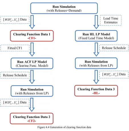
address the question above. The flowchart explaining how we generate these three clearing
function data is illustrated in Figure 4.4.
The data generation is done with three different methods. First, we generate a clearing
function data (CF1) from a simulation model with release rates equal to the demands for each
70%, 80% and 90%). We then fit the clearing functions to this data. After fitting our first
clearing functions, we run the Allocated Clearing Function LP model to obtain the release
schedules for 5 different demand levels. We then give these 5 different release schedules to
our simulation model and execute the simulation model to obtain the new [ t m
WIP , t
m
X ] data
set, which we call CF2. We now have two different clearing functions, second one obtained
by iterating on the first one. In addition to these, we also generate another clearing function
Figure 4.4 Generation of clearing function data
Figure 4.5 - Figure 4.8 present the [ t m
WIP , t
m
X ] data obtained with three different
methods (CF1, CF2 and HL) for Station1, Station 3, Station 4 and Station 7, respectively.
Run Simulation (with Releases=Demand)
[ t
m
WIP , t
m
X ] Data Lead Time
Estimates
Clearing Function Data 1
-CF1- (Fixed Lead Time Model) Run HL LP Model
Release Schedule
Run Simulation
(with Releases from LP)
[ t
m
WIP , t
m
X ] Data
Clearing Function Data 3 -HL
-Run ACF LP Model
(Clearing Func. Model)
Run Simulation
(with Releases from LP)
Clearing Function Data 2 -CF2
-[ t
m
WIP , t
m
X ] Data Release Schedule
Fitted CF1
Figure 4.5 [WIP,X] data for station 1
As explained in Section 4.1, Stations 3 and 7 are the unreliable machines which are
subject to failures, and where we expect WIP accumulation and greater variance compared to
other stations. Station 4 is the bottleneck machine, at which we can see the limit of
throughput, i.e. the capacity, is reached after a certain WIP level. Figure 4.5 also shows that
the utilization level for Station 1 is low, which results in a linear trend. Thus, basically we
expect to see the congestion behavior in a clearing function as the utilization level of the
Figure 4.6 [WIP,X] data for station 3
Figure 4.8 [WIP,X] data for station 4
As we can see from the figures above, no matter how we generate the data for
clearing function, the shape that we get is similar. We will see further evidence of the
similarity of the clearing functions derived in different ways when they are implemented in
the planning models.
4.4.2 Comparisons of Different Clearing Function Data Sets
As we explained in previous section, we collected the [ t m
WIP , t
m
X ] statistics in three
different ways in order to examine the dependence or independence of clearing functions to
production planning procedure applied. The figures showing the raw [ t m
WIP , t
m
X ] data above
procedure used. We fit two different functional forms (Srinivasan’s functional form and
Karmarkar’s functional form) to these data and then apply piecewise linearization to obtained
functions. Srinivasan et al. [10] propose a concave exponential function of the form
) 1
( )
( 2
1 e KWIP
K WIP
f = − −
(4.8)
while Karmarkar [11] suggests the following form
WIP K WIP K WIP f + = 2 1* ) ( (4.9)
The fitting methodology for these two different functional forms and piecewise
linearization is explained in detail in the next two sections. However, we will present some
charts in this section which show the slopes of the piecewise linearized clearing functions.
Figure 4.9 - Figure 4.12 present the slopes for five segments forming the clearing
functions in a comparative way for the same stations whose [ t m
WIP , t
m
X ] data presented in the
previous section. The figures have two charts next to each other: the one on the left-hand side
presents the slopes of clearing function fitted to the functional form proposed by Srinivasan
Figure 4.9 Clearing function slopes for station 1
Each different line on the charts represents different clearing function data sets (CF1,
CF2 and HL). Figure 4.9 shows the clearing function slopes for station 1 with respect to two
different functional forms which do not change significantly as the data set changes.
Figure 4.11 Clearing function slopes for station 7
Figure 4.10 and Figure 4.11 show the slopes for the unreliable stations, station 3 and
7. We still cannot see any significant difference between the slopes for three different data
sets. There is also not much difference between the two different functional form.
Figure 4.12 Clearing function slopes for station 4
As seen in Figure 4.12, the slopes for three data sets do not change significantly even
at the bottleneck station. However, we can now see a difference between the slopes of two
different functional forms, which suggest that the fitting methodology may make a difference
At this point, our evidence suggests that the form of clearing functions does not
depend significantly on the production planning procedure applied. Thus, clearing functions
are unique to the corresponding machine and no matter how we collect [ t m
WIP , t
m
X ] statistics
from that machine, it will be similar in shape.
The process of generating three different clearing function data sets is illustrated in
Figure 4.4 with a flowchart. Generating data for CF1 is the easiest of these three ways. Since
it is clear that the clearing function does not change significantly as the way of generating
data changes, we will use CF1 data in the remaining part of our thesis.
4.4.3 Clearing Function Fitting Methodology
There are two different functional forms for clearing functions in the literature.
Srinivasan et al. [10] propose a concave exponential function of the form
) 1
( )
( 2
1 e KWIP
K WIP
f = − −
(4.10)
while Karmarkar [11] suggests the alternative form
WIP K WIP K WIP f + = 2 1* ) ( (4.11)
In both of these forms, K1 and K2 are the parameters determined for fitting the
functions to the empirical data set of [ t m
WIP , t
m
X ]. K1 represents the maximum possible
output, while K2 determines the curvature of the clearing function. K1 is determined from the
empirical data and K2 is estimated by using Least Sum of Squares method. In order to
curve-fitting (data-curve-fitting) problems by minimizing the sum of squared errors. In the remainder of
this thesis, we will use (4.8) for the concave exponential functional form (Eq. 4.8) and
“Functional Form 2” (F2) for the alternative form (Eq. 4.9).
4.4.3.1 Functional Form 1 (F1)
As mentioned above, the data set CF1 was used to fit F1 with the lsqcurvefit function in MATLAB. Figure 4.13 - Figure 4.16 present the fitted clearing functions for stations 1, 3,
7 and 4, respectively.
Figure 4.13 Fitted F1 for station 1
For machine 1 we see a very good fit, because the data does not have high variance.
The curve passes through the middle of the data set, which represents the relationship
Figure 4.14 Fitted F1 for station 3
Figure 4.14 and Figure 4.15 show the fits for the unreliable stations, at which fitting
the functional form to the data is more difficult than for station 1. However, we can say that
these fits are also very good and represent the average WIP – output behavior at these
machines in a sensible way.
Figure 4.16 Fitted F1 for station 4
When we fit F1 to our bottleneck machine data, we observe that the curve does not
track the data in the congestion area, i.e. 10 < WIP < 20, which may result in capacity
overestimation problems in the ACF LP model. Since the functional form F1 tries to make
the right-hand side of the function linear after a certain WIP level is exceeded, it cannot track
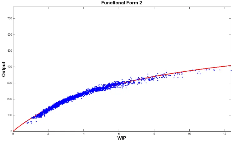
4.4.3.2 Functional Form 2 (F2)
In this section, we present the fitted F2’s for the same machines. Figure 4.17 shows
the fitted F2 for station 1. Like F1, this functional form tracks machine 1’s data very well and
is very similar to F1 results presented in the previous section.
Figure 4.17 Fitted F2 for station 1
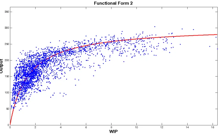
Figure 4.18 and Figure 4.19 show the fitted F2’s for the unreliable machines, which
appear to be fitted reasonably. Both functions seem to track the high-variance data by passing
Figure 4.18 Fitted F2 for station 3
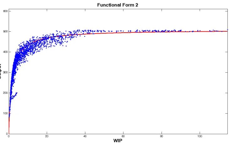
Figure 4.20 Fitted F2 for station 4
When we look at the fitted F2 for the bottleneck station, shown in Figure 4.20, we can
say that the function tracks the bottleneck machine data much better than F1. In addition to
visual interpretation, as a numerical comparison criterion, we use R2 values, which is a
descriptive measure between zero and one. The R2 value for F1 is 0.7902, while it is 0.9369
for F2, which also supports that F2 tracks the data better than F1 statistically. In this form,
the congestion area behavior of expected WIP and output appears to be represented more
accurately. In addition, it also follows the data for high WIP levels where the resource is
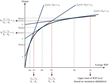
4.4.4 Piecewise Linearization
In order to use the clearing functions in our linear programming model of the ACF
formulation, we need to approximate the fitted concave curves by applying outer
linearization method. Thus, the clearing function can be represented by a set of linear
constraints in our production planning LP model.
We must first determine the number of lines (segments) that we will use to
approximate the clearing functions before piecewise linearization. There is a tradeoff
between the computational time for optimization model and accuracy of the approximation as
we increase the number of the lines. Turkseven [23], conducted experiments with different
number of segments at the clearing functions. It was found out that 3 lines would be
sufficient to express a clearing function, because the improvement in solution quality
(minimized area that is the difference between clearing function curve and line segments) is
minimal when the number of segments is increased. For that reason, we will use 3-segment
![Figure 4.5 [WIP,X] data for station 1](https://thumb-us.123doks.com/thumbv2/123dok_us/1424896.1175005/48.612.133.504.148.384/figure-wip-x-data-for-station.webp)
![Figure 4.7 [WIP,X] data for station 7](https://thumb-us.123doks.com/thumbv2/123dok_us/1424896.1175005/49.612.132.504.152.374/figure-wip-x-data-for-station.webp)
![Figure 4.8 [WIP,X] data for station 4](https://thumb-us.123doks.com/thumbv2/123dok_us/1424896.1175005/50.612.133.502.145.384/figure-wip-x-data-for-station.webp)