Electronic Theses and Dissertations Theses, Dissertations, and Major Papers
2012
An Exploration of the Feasibility of FPGA Implementation of Face
An Exploration of the Feasibility of FPGA Implementation of Face
Recognition Using Eigenfaces
Recognition Using Eigenfaces
Vinod Anbalagan
University of Windsor
Follow this and additional works at: https://scholar.uwindsor.ca/etd Recommended Citation
Recommended Citation
Anbalagan, Vinod, "An Exploration of the Feasibility of FPGA Implementation of Face Recognition Using Eigenfaces" (2012). Electronic Theses and Dissertations. 8122.
https://scholar.uwindsor.ca/etd/8122
This online database contains the full-text of PhD dissertations and Masters’ theses of University of Windsor students from 1954 forward. These documents are made available for personal study and research purposes only, in accordance with the Canadian Copyright Act and the Creative Commons license—CC BY-NC-ND (Attribution, Non-Commercial, No Derivative Works). Under this license, works must always be attributed to the copyright holder (original author), cannot be used for any commercial purposes, and may not be altered. Any other use would require the permission of the copyright holder. Students may inquire about withdrawing their dissertation and/or thesis from this database. For additional inquiries, please contact the repository administrator via email
Implementation of Face Recognition
Using Eigenfaces
by
Vinod Anbalagan
A thesis
Submitted to the Faculty of Graduate Studies the Department of Electrical and Computer Engineering
in Partial Fulfillment of the Requirements of the Degree of Master of Applied Science at the
University of Windsor
Windsor, Ontario, Canada
I hereby declare that I am the sole author of this thesis. This is a true copy of the thesis, including
any required final revisions, as accepted by my examiners.
Biometric identification has been a major force since 1990's. There are different types of
approaches for it; one of the most significant approaches is face recognition. Over the
past two decades, face recognition techniques have improved significantly, the main
focus being the development of efficient algorithm. The state of art algorithms with good
recognition rate are implemented using programming languages such as C++, JAVA and
MATLAB, these requires a fast and computationally efficient hardware such as
workstations.
If the face recognition algorithms could be written in a Hardware Description Language,
they could be implemented in an FPGA. In this thesis we have choose the eigenfaces
algorithm, since it is simple and very efficient, this algorithm is first solved analytically,
and then the architecture is designed for FPGA implementation. We then develop the
Verilog module for each of these modules and test their functionality using a Verilog
Simulator and finally we discuss the feasibility of FPGA implementation.
Implementing the face recognition technology in an FPGA would mean that they
would require relatively low power and the size is drastically reduced when compared to
the workstations. They would also be much faster and efficient, since they are
There are several people who deserve my sincere thanks for their generous contributions
to this project. First and foremost I would like to express my deepest gratitude and
appreciation to Dr. Jonathan Wu and Dr. Mohammad Khalid, my supervisors for their
invaluable guidance, encouragement and support over the years. Their generosity,
wisdom, empathy and professionalism helped me complete this thesis, would also like to
thank Dr. Tepe and Dr. Zhang for their invaluable advice.
Secondly, I would like to express my gratitude to Dr. Nihar Biswas, who
personally helped me overcome my personal difficulties. Also I am very thankful to Mrs.
Andria Ballo, for always being there for me and for all the engineering souls in distress,
assisting them with her guidance, support and friendly approach.
Next, I would like to thank my senior and friend Mohan Thangarajah, for
constantly encouraging me and helping me whenever I was in need. His company
through the university years would be cherished, especially our 7/11 and Tim Hortins
coffee breaks whilst staying up all night for working on our projects in our office, lab and
library.
Finally, I would like to thank my parents A. Premalatha and R. Anbalagan, my
brother A.Vivek, for all their understanding, support and sacrifices over the past couple
Fifi Dyne, Lorena Marie, James 0. Lepp, Steven O. Lepp, Jeni Robertson, Ricki Oltean,
Kirsta and Chris Konrad, Gina, Chelsea and Gerry Lepp, your support, motivation and
Abstract iv
Acknowledgment v
Dedication vii
List of Figures xiii
List of Tables xvi
List of Abbreviations xvii
1 Introduction 1
1.1 Face Recognition 1
1.2 Eigenfaces 2
1.3 Problem Statement 3
1.4 Objectives 4
1.5 Motivation 4
1.6 Thesis Organization 5
2 Biometric Recognition 7
2.1 Introduction 7
2.2 What is Biometrics? 7
2.3 Need for Biometric System 8
2.4 Types of Biometric Recognition 9
2.5 Application of Biometric Systems 10
2.6 Advantages of Biometric Systems 11
3 Face Recognition 13
3.3 Disadvantages of Other Biometric Systems 14
3.4 Advantages of Face Recognition System 14
3.5 Evolution of Face Recognition 15
3.6 Applications of Face Recognition 18
3.7 Face Detection 18
3.7.1 Face Detection Scenarios 19
3.7.2 Face Detection Methods 20
3.7.2.1 Knowledge Based Methods 20
3.7.2.2 Template Matching 20
3.7.2.3 Appearance Based Method 21
3.8 Face Extraction 21
3.9 Face Classification 22
3.10 Different Approaches in Face recognition 23
3.10.1 Appearance Based Approach 24
3.10.1.1 Linear Analysis 24
3.10.1.1.1 Principal Component Analysis 25
3.10.1.1.2 Linear Discriminant Analysis 25
3.10.1.1.3 Independent Component Analysis 26
3.10.1.2 Non-Linear Analysis 26
3.10.2 Model Based Approach 26
3.10.2.1 2D Approach 27
3.10.2.1.1 Elastic Bunch Graphing 27
3.10.2.1.2 Active Appearance Model 28
3.10.2.2.1 3D Morphable Models 28
3.10.3 Piecemeal / Holistic Approach 29
3.10.3.1 Hidden Markov Model 29
3.11 Face Recognition Database 30
3.12 Difficulties in Face Recognition 30
4 Eigenfaces 32
4.1 Introduction 32
4.2 Principal Component Analysis 32
4.3 Background Mathematics 33
4.3.1 Standard Deviation 33
4.3.2 Variance 34
4.3.3 Co-Variance 34
4.3.4 Eigenvectors and Eigenvalues 35
4.4 PCA Example Calculation 36
4.5 PCA in Face Recognition 43
4.6 Eigenfaces 44
4.7 Eigenfaces Approach 46
4.8 Assumptions in EA 49
4.9 EA 49
4.10 Face Space 54
5 Proposed Architecture for FPGA Implementation of EA 57
5.1 Introduction 57
5.2 Data Representation 58
5.4.1 Phase I 62
5.4.1.1 RAM Controller 64
5.4.1.2 RAM Blocks 67
5.4.1.3 Controller to Control Location and Position 69
5.4.1.4 Pipelining 71
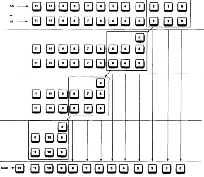
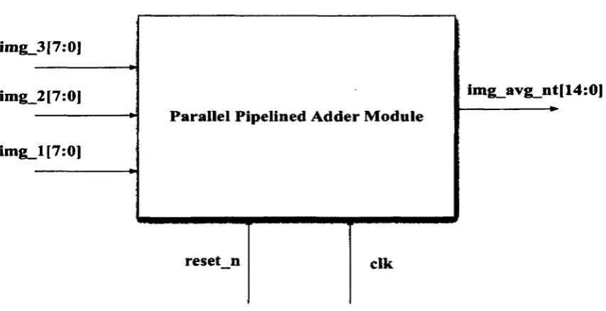
5.4.1.5 Parallel-Pipelined Adder 73
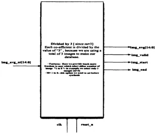
5.4.1.6 Divider Module 75
5.4.1.7 Bit Check Module 81
5.4.1.8 Pipelined Adder 82
5.4.1.9 Multiplier 85
5.4.1.10 MATLAB Module 88
5.4.2 Phase II 90
5.4.2.1 Multiplier 92
6 Simulation and FPGA Implementation Issues 103
6.1 Introduction 103
6.2 Simulation 103
6.2.1 Basic Simulation Flow 103
6.2.2 Simulation Result 105
6.2.2.1 Parallel-Pipelined Adder Module 105
6.2.2.2 Divide by - 3 Module 106
6.2.2.3 Read and Write Address Generator Module 107
6.2.2.4 Read and Write Data to RAM Module 107
7 Conclusion and Future work 111
7.1 Dissertation Summary Ill
7.2 Future Work 112
References 113
1.1 Eigenface 2
2.1 Types of Biometric Recognition 10
3.1 Sub-Routines in Face Recognition System 18
3.2 Face Recognition Approaches 24
4.1 Plot of Original Data 37
4.2 Mean Adjusted Data 38
4.3 Mean Adjusted Data with Eigenvectors 39
4.4 Final Data with Eigenvectors 40
4.5 Comparison between Original Data and Final Data 42
4.6 PCA in Face Recognition 44
4.7 Flowchart - Eigenfaces 48
4.8 Eigenfaces Concept 49
4.9 Face Images from AT&T Database 50
4.10 Average Face 51
4.11 Difference Face 51
4.12 Eigenfaces 53
4.13 Image Space and Face Space 55
4.14 Different Possibilities of Face Space and Face Class 56
5.1 Proposed Architecture for Eigenfaces 61
5.3 RAM Controller 66
5.4 RAM Blocks 67
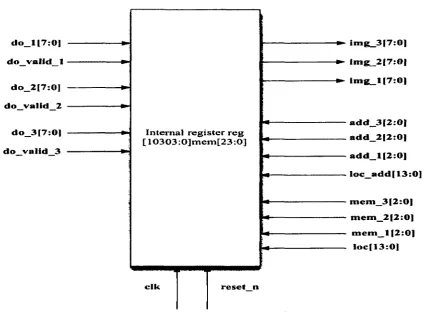
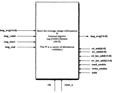
5.5 Internal Register 69
5.6 Controller to Control the Address Location and Position 70
5.7 Pipelined Addition of'Two' 12bitData 72
5.8 Parallel-Pipelined Adder 73
5.9 Divide by - 3 Module 76
5.10 Average Information Module 77
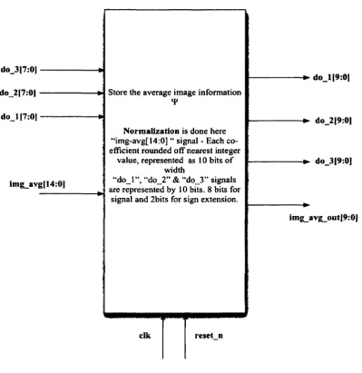
5.11 Normalization Module 78
5.12 Controller to Control the Address Location and Position 79
5.13 Bit Check Module 82
5.14 Pipelined Adder 83
5.15 Difference Face 83
5.16 Multiplier Module - ('A' Matrix and 'AT' Matrix) 86
5.17 L Matrix - Normalization Module 86
5.18 MATLAB Module 89
5.19 Architecture Data Flow - Phase II 90
5.20 Multiplier Module - ('A' matrix and Eigenvectors Vi,V2and V3) 92
5.21 Internal Register - ('U' and 'UT' Matrix) 93
5.22 Bit Check Module 96
5.23 Parallel-Pipelined Adder - (Average Face and Unknown Face) 97
5.24 Parallel-Pipelined Adder - (Average Face and known Face) 98
5.27 Pipelined Adder for Weight Vector 101
5.28 Compare and Display Module 101
6.1 Basic Simulation Flow 104
6.2 Parallel-Pipelined Adder Interface Module 105
6.3 Divide by 3 - Interface Module 106
6.4 Read and Write Address Generator Module Interface 107
4.1 Original Data 36
4.2 Mean Adjusted Data 37
4.3 Final Data 40
5.1 RAM Controller - Port Names and Description 64
5.2 Internal Register - Port Name and Description 68
5.3 Parallel-Pipelined Adder - Port Name and Description 75
5.4 Divide by - 3 Module - Port Name and Description 75
The notation used in this thesis is as follows. In general, a scalar element of a vector is denoted as
v, e v, Which is read as " the i4 element of vector v with indexing of vectors starting at i = 1
and ranging to the length of the vector. All vectors are assumed to be column vectors. Some
commonly used operators, symbols and abbreviations are listed below.
Abbreviations Definition
(•)
T Transpose OperatorN x N Height (N) and Width (N) of an Image
X Mean of x
I Identity Matrix
D Dimension
SD Standard Deviation
V Variance
Cov Covariance
C Covariance Matrix in Eigenfaces Algorithm
L Dimensionality Reduced Covariance of Eigenfaces Algorithm
U Eigenvector of Covariance Matrix 'C'
V Eigenvector of Covariance Matrix 'L'
X
Eigenvaluen
Weight Vector£rec Smallest Euclidean Distance
0
rec Heuristically Chosen Valuer
An Image in the Database® Difference face vector
M Total Number of Images in the Database
K Top Most Significant Eigenfaces
MATLAB Matrix Laboratory
HDL Hardware Description Language
FPGA Field Programmable Gate Array
ID Identification
E-Passport Electronic Passport
DOD Department of Defense
MIT Massachusetts Institute of Technology
FERET Face Recognition Technology
DARPA Defense Advanced Research Product Agency
FVRT Face Recognition Vendor Test
PCA Principal Component Analysis
LDA Linear Discriminant Analysis
ICA Independent Component Analysis
FBG Face Bunch Graphing
AAM Active Appearance Model
HMM Hidden Markov Model
FRGC Face Recognition Grand Challenge
AT&T American Telephone & Telegraph
CAS-PEAL Chinese Academy of Science - Pose, Expression, Accessory and Lighting
PICS Psychological Image Collections
RMA Royal Military Academy
RAM Random Access Memory
LSB Least Significant Bit
MSB Most Significant Bit
EA Eigenfaces Algorithm
Introduction
1.1 Face Recognition
Face recognition in humans has always been an enigma, for we can recognize a face with
facial hair, occlusion, even after several years of separation and in worst possible lighting
conditions. For two decades now researchers, not only from the field of computer vision
but also psychologists and neurologists, have been trying to emulate this ability using
machines, so far we only know that the temporal lobe in the brain is partly responsible for
face recognition, damage to this region would result in a person losing his ability to
recognize faces, and this condition is called prosopagnosia. Even after this condition has
occurred, the perception of face remains unchanged because the human mind would use
its hearing ability and cognitive ability to analyze the voice and gait of a person for
recognition, so emulating such an ability will be an herculean task even with the latest
available technology. This challenge is one reason why face recognition has caught the
1.2 Eigenfaces
The concept of eigenfaces is similar to Fourier decomposition, which is one of the most
fundamental ideas in mathematics and signal processing. A Fourier series decomposes
periodic signals into sum of (possibly infinite) set of simple oscillating functions namely
sine and cosines.
Eigenfaces technique represents a face as linear composition of the base images
also known as 'eigenfaces' or 'eigenpictures', these eigenfaces are basically a set of
eigenvectors used in computer vision problem, they are generated by performing a
mathematical procedure called 'Principal Component Analysis' [Joll 02] on a large set of
human face images. In mathematical terms, we are finding the eigenvectors of the
covariance matrix of a set of faces, where these faces are treated as a vector in a high
dimensional space. The characteristic features from each face contributes to the
eigenvectors, which can be represented as a ghostly face as show in Figure 1.1, we call
this as an eigenface.
The approach of using eigenfaces for recognition was developed by Sirovich and Kirby
(1987) at Brown University [Kirb 87], later was expanded and developed by Matthew
Turk and Alex Pentland [Turk 91] [Pent 91], which was considered as the first successful
model of automated face recognition technology.
1.3 Problem Statement
Face recognition techniques have improved significantly. The focus of face recognition
has been to develop the most efficient algorithm; researchers have been striving to
develop this elusive algorithm with highest recognition rate. Face recognition algorithms
require computationally efficient and fast hardware with high storage capabilities such as
mainframes, workstations and server desktop computers.
If we deploy face recognition technology; we would require the best and efficient
workstations stationed at every entry points under human supervision, this could be very
costly and is not feasible in places like a huge organizations, storage facilities,
multistoried parking areas, residential complexes, warehouses, etc. The majority of the
areas would go uncovered and vulnerable since they would have many entry points. In
this thesis we explore the feasibility of implementing face recognition technology in a
FPGA, which would drastically reduce the size and would only require relatively low
power without compromising on recognition rate or speed. The reduction in size would
imply that it could be used in places where we would normally hesitate to use a
1.4 Objectives
The work presented in this thesis has the following objectives.
1. Investigate new and existing algorithms and choosing a computationally efficient,
simple and accurate method.
2. Propose a feasible architecture for FPGA implementation based on the chosen
algorithm.
3. Developing Verilog HDL module for each individual module and test its
functionality using a Verilog simulator.
1.5 Motivation
Biometric signature is very distinct in verifying identities of an individual; they cannot be
guessed, stolen, forged or lost.
Biometric identities are derived from physiological characteristics such as face,
fingerprint, finger geometry, hand geometry, iris, palm, vein, retina and voice. Behavioral
traits such as gait, signature and keystroke dynamics can also be used in establishing
biometric identity.
Face recognition seems to offer several advantages over other biometric methods;
also face recognition can be done passively, where the subject need not even raise their
finger, but the face recognition technologies [Cogn 10] [Ayon 10] [Auro 08] that are
available now, require computationally efficient workstations and servers, since the
algorithm used are very complex and computationally intensive, along with the power
recognition rate. This hurdle could be crossed if we could implement face recognition
algorithm on an FPGA.
Currently face recognition algorithms are implemented programming languages
such as C++, JAVA, MATLAB, Python and Mathematica. They are yet to be written in a
Hardware Description Language (HDL). This thesis aims at exploring the feasibility of
FPGA implementation of face recognition using the best and the most efficient algorithm
implemented using Verilog HDL.
1.6 Thesis Organization
Developing from the introduction in Chapter 1, Chapter 2 summarizes the biometric
systems, types of biometric system, applications and advantages of biometric system.
Chapter 3 covers face recognition technology's development though history, face
detection, extraction and classification process, popular face recognition approaches, the
difficulties involved in implementing face recognition technology and the available
database for face recognition.
Chapter 4 of this thesis provides a thorough background, mathematical
conceptualization and algorithm of principal component analysis and eigenfaces. The
chapter continues with a discussion on the assumptions and the steps involved in the
algorithm by presenting a detailed analysis of eigenfaces calculations using a small
example.
Chapter 5 builds on the foundation laid in Chapter 4; it proposes a flexible
architecture for implementing eigenfaces, each and every module from the architecture
Chapter 6 presents the ModelSim Simulation results of the functionality of the
architectural blocks and discusses the feasibility of FPGA Implementation and related
issues.
Biometric Recognition
2.1 Introduction
Biometrics consists of methods for uniquely identifying individuals based on physical
and behavioral traits. This Chapter begins by discussing the history of biometrics and the
need for biometrics. We also discuss the different types of biometrics and finally the
advantages and applications of biometrics.
2.2 What is Biometrics?
The term "Biometrics" is derived from the Greek word "Bio" (life) and "metrics" (to
measure). Automated biometric system [Coun 06] has only been available over the last
few decades due to significant advances in technology.
Biometric recognition, however fancy the name sounds, was conceived before
thousands of years ago. In the earliest civilizations the cave walls were said to be adorned
with paintings and alongside these paintings there were numerous handprints, which were
believed to be tamper proof signature, by its creators. Face recognition was used by the
early civilizations to categorize an individual between known and unknown. Human to
patterns such as voice and gait. These physiological and behavioral patterns recognition
were collectively known as biometric recognition.
2.3 Need for Biometric Systems
During the mid 1800s there was rapid growth of cities due to industrial revolution. As
more and more people were migrating towards the cities, unrest and chaos was a common
scene, this made it more and more difficult for the justice system, to keep track of the
repeated offenders. They used a formal system that recorded the offences along with the
identity trait of the offender; this marked the birth of the official biometric system.
Personal security is being treated with utmost importance these days and rightly
so, since the identity thefts are on rise. Unconventional recognition techniques such as
password and ID card are based on "what you know?" and "what you have?" In contrast
Biometric technology is based on "who you are?" It is derived from physiological traits
such as face, fingerprint, iris, palm-print, voice and behavioral traits such as signature,
gait and keystroke. This technology is extremely difficult to duplicate, steal, copy,
misplace or forge.
Since the advent of Internet, everything has gone online, including our day-to-day
activities such as online banking, social networking, online shopping etc. All our online
activities start with logging in and logging off the network with our user ID and
password. These could be easily hacked, stolen and guessed. Once this information falls
anyone. Therefore to avoid such situations a good solution is to implement an effective
biometric system.
2.4 Types of Biometric Recognition
There were two approaches to the early biometric system, the first approach was called as
Bertillon System of Measuring Various Body Dimensions, and this originated in France.
These measurements were written on cards that were sorted by height, weight, arm's
length etc., this field was called anthropometrics. The second approach was the method of
taking fingerprint from the index finger; this was introduced in Asia, Europe and South
America by 1800s. This method was based on the ridges and the finger print pattern on
the index finger.
The later half of the 20th century saw the much more advanced phase of biometric
system, which was helped by development in Computer Systems and Technology, the
biometric system could be categorized [Saw 11] into two groups, Physiological
characteristic and Behavioral characteristics, different methodologies have been
jC
Figure 2.1: Types of Biometric Recognition
2.5 Applications of Biometric Systems
The following are some of the applications of biometric systems.
1. Biometric Fingerprint Identification Systems are widely used in forensics for
criminal identification.
2. Biometrics are widely used for Physical Access Control
3. Logging into Computers
7. To verify customers during transactions via telephone and Internet.
8. E-passports are a work in progress for issue in near future, which has an
embedded chip containing the holder's facial image and other traits.
2.6 Advantages of Biometric Systems
The following are some of the advantages of biometric systems
Uniqueness:
It is impossible for two people to share the same biometric data, so biometric
systems are designed around an individual and unique characteristic.
Cannot be Lost:
A Biometric data could never be lost, unless the individual is involved in a
terrible accident.
Cannot be Copied or Guessed:
Biometric data cannot be forged or shared or guessed, since the biometric data are
physiological attributes.
The fact that biometric system needs "You" to authenticate that the subject is you is the
Face Recognition
3.1 Introduction
Face recognition is a form of biometric identification, which uses facial features as the
basis for identification. This chapter covers face recognition, its development through
history and the different areas of application. It also talks about the steps involved in face
recognition; such as face detection, feature extraction and face classification. Finally, it
describes the different types of approaches for face recognition, list of available face
databases and the difficulties in face recognition.
3.2 Primary Tasks of Face Recognition
Face recognition is used for two primary tasks, which are as follows
Verification: (one to one matching)
When an individual presents an identity, the system verifies whether the
individual is who he claims to be.
Identification: (one to many matching)
If an image of an unknown individual should be identified, the system verifies the
3.3 Disadvantages of Other Biometric Systems:
When using other biometric systems, there are a few disadvantages, which are as follows
1. Finger print of people working in chemical industry can be affected
2. Voice recognition system would fail when a person has a sore throat and also
voice of a person would change with age, which would complicate the system.
3. For people with diabetes, the eyes would get affected resulting in failure to
authenticate, also iris recognition is very costly to implement.
4. Digital Signatures could be modified or forged.
The above disadvantages could be overcome by using face recognition method with an
effective algorithm.
3.4 Advantages of Face Recognition System:
Face recognition system is advantageous over other biometric systems; some of the
advantages are as follows,
1. Almost all of the biometric systems require the user to perform an action like
placing their hand or finger for finger print reading, speaking into the microphone
for voice recognizer etc. However face recognition does not require any explicit
action from the user.
2. Face recognition technology is cheaper when compared to other biometric
systems.
4. Face recognition system does not cause any health risk to the user, whereas other
biometric technology that requires multiple users to use the same equipment can
potentially expose them to germs from previous users.
3.5 Evolution of Face Recognition
Face recognition technology has been extensively researched over the years. Researchers
are still working on algorithms that can provide high accuracy and portability. Face
recognition is a challenging task because of factors like change in expression, scale,
location, occlusion, pose and lighting conditions.
Many algorithms have evolved over the years [Coun 06] The Earliest Work on
Face Recognition was from the Field of Psychology during the 1950s. "The perception of
people, a handbook of social psychology" [Tagi 54] by J.S Bruner and R. Tagiuri.
Engineer's interest in face recognition resulted in the first semi automated face
recognition system during the 1960s. Woodrow W. Bledose and other researchers
developed the first semi automated face recognition system at Panoramic Research Inc.,
in Palo Alto, California [Bled 66]; the US Department of Defense (DOD) funded this
work. This system required human interference to locate the feature points such as eyes,
nose and mouth in photographs and the distance and ratios are calculated so that it can be
later compared to test image for recognition.
During the 1970s face recognition moved forward from semi automation. A. J.
compared. In 1973 face recognition with template matching was introduced. Martin A.
Fischler and Robert A. Elschlager [Fisc 73] measured the similar features as in the earlier
papers but they made it automatically, they described an algorithm that used local feature
template matching approach. In the same year Kanade developed the First Fully
Automated Face Recognition system [Kana 73]. Kanade used pattern classification
technique to match test faces to a known set of faces, this was a purely statistical
approach. Template matching technique was improved during the 1980s. Mark Nixon's
[Agua 02] Eye spacing measurement improved template-matching approach by
introducing 'deformable templates'.
The first semi-automatic facial recognition system was deployed during 1988.
The Lakewood division of Los Angeles county sheriffs department began using
composite drawings of suspects to conduct a Mug shot database search using this system.
In the same year eigenfaces technique was developed for face recognition. L. Sirovich
and M. Kirby [Kirb 90] applied Principal Component Analysis, a linear algebra technique
on face images, they represented an image in a lower dimension as principal component
vectors without losing much information, and then reconstruction them.
In 1991 face detection technique was mastered, making real time face
Recognition was possible, Matthew Turk and Alex Pentland of MIT [Turk 91] [Pent 91]
extended the work on eigenfaces technique and made this a state of art face recognition
technique; this was the first successfully available industrial application, this paved way
for a new era in Face recognition systems. In 1993 FacE REcognition Technology
(FERET) program was initiated. The Defense Advanced Research Products Agency
Technology (FERET) [Phil 97] in an effort to develop face recognition algorithm and
technology to commercialize the product. Face Detection based on Neural Networks was
introduced in 1988. Henry A. Rowley, Shumeet Baluja and Takeo Kanade [Rowl 98]
came up with face detection technique using Neural Networks.
Face Recognition using Elastic Bunch Graph Method was introduced in 1999,
Laurenz Wiskott, Jean-Mark Fellous, Norbert Kruger, Christoph Von Der Malsburg
[Wisk 97] presented a system for recognizing human faces using Gabor wavelets
transform on images. A face graph is created from an image, it consists of sparse
collection of jets at the edges where eyes, nose mouth are located, the face bunch graph
has a stack like structure and combines graphs of individual sample faces. Comparing the
similarities between the graphs can recognize a new face.
In 2000 First Face Recognition Vendor Test was held. Multiple US Government
agencies sponsored the Face Recognition Vendor Test (FVRT) [Phil 03], this served as
the first open large-scale technology evaluation of multiple commercially available
biometric systems.
In the following decade face recognition systems has seen several changes and is being
3.6 Applications of Face Recognition
There are numerous areas where face recognition could be employed; a few are outlined
below.
1. Criminal Justice system - Mug shot database, witness face reconstruction, video
surveillance and Forensics reconstruction of face from remains.
2. Network security - User authentication, database access, e-commerce and online
banking.
3. National Security - National IDs, Voter Registration, Border Crossing, etc.,
4. Personal Security - Home Video Surveillance, Driver Monitor system.
5. Access Control - Access control in areas like Warehouse, Seaports and Airports.
6. Entertainment - PlayStation, Digital cameras, etc.
3.7 Face Detection
Facial Recognition System [Grgi 07] is a whole package that consists of steps such as
face detection, feature extraction and face classification. Figure 3.1 illustrates the steps
involved a face recognition system
Face Detection Feature
Extraction Face Classification
Figure 3.1: Steps in Face Recognition System
The first step in any face recognition system is the detection of faces in images, since the
recognition algorithm would not require to detect faces in images, since the images are
normalized and fit to size according to the need of the algorithm, incase if the image is
too complex and is not normalized then we might have to detect the face from the image,
these images are mostly taken under uncontrolled environments, the following are the
factors that challenge face detection
1. Pose variation
2. Facial Expression
3. Background Environment
4. Occlusion
3.7.1 Face Detection Scenarios
There are two basic scenarios in face detection, first is when an image is taken under
controlled condition; the face is detected using edge detection technique. Second scenario
is when an image is taken under uncontrolled condition [Leun 95], if it is a color image
[Naka 96] then the skin color [Kend 96] could be used to identify the face, incase if it's a
grey scale image then the position of features like eyes, nose and mouth could be
3.7.2 Face Detection Methods
Face detection methods [Ahuj 02] are detected in to four categories, which are as follows.
3.7.2.1 Knowledge Based Method
In knowledge-based method [Teka 98] we try to apply a set of rules, which are derived
from our knowledge of faces, some of the rules are, a face usually has two symmetrical
eyes, the distance between the eyes, the color difference between the cheeks and the area
under the eyes, etc., while making these rules we have to make sure that they are not too
vague (generalized), if they are then there would be many false positives, on the other
hand false negatives would be generated if the rules are too fine (detailed). This method
of face detection has its own limitations and the detection rate depends on the rules
applied for this method.
3.7.2.2 Template Matching
Template matching [Pogg 92] method tries to define a face as a function; each feature
such as eyes, nose, mouth and ears can be defined independently in a face. Face contour
and relationship between different templates are identified as patterns, these standard
patterns are compared to images to detect faces, this type of detection is very simple to
implement, but these methods are limited to faces that are frontal and un-occluded,
3.7.2.3 Appearance Based Method
Appearance based/ View based [Lew 96] [Pogg 98] method rely on techniques from
statistical analysis and machine learning methods, Appearance based method is said to
have a probabilistic nature, such that it finds if an image vector would belong to a face or
not, it depends on the discerning ability to identify a face class from a non face class.
Comparing with the other two face detection methods, appearance based method
has higher detection rate, few tools [Mite 96] that are based on appearance-based
methods [Turk 91] [Pent 91] [Sama 93] [Guo 00] [Phil 99] [Osun 97] [Sebe 02] are
listed below
1. Eigenfaces
2. Neural Networks
3. Hidden Markov Models
4. Naive Bayes Classifier
5. Support vector machines
3.8 Feature Extraction
Facial features [Craw 06] [Yow 97] are the essence of a face, for they make a face
distinct from one another, many face recognition algorithms incorporate feature
extraction, this must be optimized so that it takes much less memory and has reduced
An input face image is reduced to a feature set; this feature set is reduced to a
subset by discarding the non-relevant features and choosing the best of the feature set, the
following are few methods [Rowl 98] of feature extraction.
1. Generic method based on lines, curves and edges
2. Principal Component Analysis
3. Template based method
4. Neural Network based method
5. Self Organizing Maps
The number of features that are to be extracted from a face should be carefully chosen, if
it is too low, this might lead to loss in accuracy, if it is too high, then it might result in
more false positives and might take more memory and processing time.
3.9 Face Classification
Face classification is the step that follows feature extraction; classifiers when used in
combination with other classifiers outperform individual classifiers.
The basic classifier [Jain 00] is the one that classifies face based on similarity, it
classifies the similar class from the non-similar class, and an example of such classifier is
Euclidean Distance Classifier [Mite 96], some feature extractors could also be used as a
classifier, following are the list of few of the classifiers
1. Euclidean Distance Classifier
2. Vector Quantization
3. Self Organizing Maps
Since a classifier could be used in combination with other classifiers [Roli 01] [Kitt 98],
we can use a classifier to recognize the eyes, another classifier to recognize the nose and
another classifier to recognize the mouth, all these classifiers could be combined [Tuly
08] [Wang 03] [Heis 03] for an effective classification, these combinations could be
divided into three types
1. Parallel - All the classifiers are executed independently, and then they are finally
combined together.
2. Serial - Classifiers run one after another, where each classifier would refine the
previous classifier result.
3. Hierarchical - Classifiers are arranged in a tree like structure.
Choosing the best classifier impacts the processing speed and the accuracy, choosing a
very simple classifier would produce less accurate but a quicker result, whereas choosing
a complex classifier would produce a more accurate result but it takes more processing
time, so its important to strike the right balance to choose the best classifier.
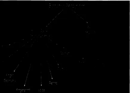
3.10 Different Approaches in Face Recognition
Face Recognition methods [Arab 09] [Rose 03] evolved over time, it can be seen as a
process, which includes many steps. These steps could overlap or change their order to
Figure 3.2: Face Recognition - Approaches
3.10.1 Appearance based Approach
An Image is considered to be a point in high dimensional vector space; an appearance
based or view based approach uses statistical technique to analyze the distribution of
image vector in the vector space and classifies the essential features for efficient
recognition. The Appearance based method can be divided into Linear and Non-Linear
Analysis.
3.10.1.1 Linear Analysis
Three of the widely used linear analysis classifications are
1. Principal Component Analysis (PCA)
3. Independent Component Analysis (ICA)
3.10.1.1.1 Principal Component Analysis
PCA is one of the most widely used classifiers; it is based on Karhunen-Loeve
transformation [Kirb 87] [Pent 97] [Turk 01]. PCA performs a dimensionality reduction
by extracting the principal components of high dimensional data, these principal
component vectors defines the face space, which is a subspace in the image space.
The face images are projected onto the face space and their weights are identified,
and the test image is projected onto the face space, the weight coefficient of the test face
image is compared with the weights of the face images from the database, using a
distance classifier will give us the closest possible match to the test face.
3.10.1.1.2 Linear Discriminant Analysis
Linear Discriminant Analysis [Belh 97] finds the vector in the underlying space that best
discriminates the classes, for all samples of all classes the between-class scatter matrix
and within-class scatter matrix are defined.
LDA is closely related to PCA, it explicitly attempts to model the difference
between the classes of data; PCA on the other hand does not take into account any
3.10.1.1.3 Independent Component Analysis
Independent Component Analysis [Bart 02] [Como 92] [Liu 99] minimizes both second
order and higher order dependencies in the input data and attempts to find the basis along
which the data are statistically independent. ICA is generalization of PCA.
3.10.1.2 Non Linear Analysis
The face manifold in subspace need not be linear; kernel methods are a generalization of
linear methods.
Linear analysis are not very sensitive to relationships among multiple pixels in an
image, to extract the non linear features of the image linear analysis methods was
extended to non linear analysis [Yang 02] such as Kernel PCA [Scho 98] [Zhou 04],
Kernel ICA [Jord 02] and Kernel LDA.
3.10.2 Model based Approach
A model of human face is constructed to capture the features, facial variations and texture
of a face.
Prior knowledge of facial features are used to construct a model, a model based
approach [Lani 95] derives distance and relative positions from the placement of facial
elements such as eyes, nose, ears and mouth, a constructed model is often called as
Morphable Model, a model based approach is divided into two types
1. 2D Approach
3.10.2.1 2D Approach
Two-dimensional approach can be divided into two categories
1. Elastic Bunch Graphing
2. Active Appearance Model
3.10.2.1.1 Elastic Bunch Graphing
A face is represented as a graph, considering the fact that all human faces have the
similar topographical structure, the graph is constructed with nodes positioned at eyes,
nose edge, mouth, etc., these positions are called as fiducial points, the edges are labeled
with a 2D distance vector, with these vectors a face graph is constructed.
The face bunch graph has a stack like structure and it combines graphs of
individual sample faces, it is crucial that the individual graphs all have the same structure
and that the nodes refer to the same fiducial points.
A jet is a condense and robust representation of a local grey value distribution, it
is based on Gabor Wavelet Transform, which is a convolution with a family of complex
gabor wavelets having the shape of plane waves restricted by Gaussian envelope
function. All jets referring to the same fiducial points, for example, all the right eye jets
are bundled together in a bunch, the right eye bunch might contain a male eye, a female
eye, both closed and open etc., from which we can select any jet as an alternate
description. To recognize a new face by elastic bunch graph matching [Wisk 97] [Kela
between the graph of this face and the graph of every face stored in Face Bunch Graph
(FBG).
3.10.2.1.2 Active Appearance Model
An Active Appearance Model (AAM) [Tayl 01] [Walk 00] is an integrated statistical
model, which combines a model of shape variation with a model of the appearance
variation in a shape-normalized frame.
The Active Appearance Model is constructed based on a set of labeled images,
where landmark points are marked on each example face at key positions to describe the
facial features, models are combined together by using linear analysis method such as
PCA. Matching to an image involves finding model parameters; AAM fitting is applied
to seek a set of model parameters, which minimize the differences between the image and
a synthesized model example projected into the image.
3.10.2.2 3D Approach
Human face is a surface lying in the 3D space, thus a 3D model is more suitable for
representing faces. Once such method based on 3D approach [Zhan 09] [Bron 04] is 3D
Morphable Model.
3.10.2.2.1 3D Morphable Models
3D models have stronger ability to minimize the problems of head, pose and illumination,
The Morphable face model is based on a vector space representation of faces,
which is constructed such that any convex combination of shape and texture vectors of a
set of examples describes a realistic human face.
3.10.3 Piecemeal/Holistic Approach
Faces can be identified with minimal information; some algorithms would require only
the independent information for face recognition unlike other algorithms that uses the
whole face or the relationship between individual features and the face. Early researchers
tried to use very little but relevant features [Mais 92] for face recognition. Although
feature processing is important, relation between features is also important. This is one of
the reasons why most face recognition follow holistic approach, one such model that is
based on holistic approach [Nixo 85] is Hidden Markov Model (HMM)
3.10.3.1 Hidden Markov Model
Hidden Markov Models [Sama 93] [Nefi 98] [Raja 98] are a set of statistical models used
to characterize the statistical properties of a signal. Faces are intuitively divided into
regions such as eyes, nose, mouth etc., these regions can be associated with the states of a
Hidden Markov Model, since HMMs require a one dimensional observation sequence
and images are two dimensional, the images should be converted into one dimension
3.11 Face Recognition Database
Face recognition algorithms keeps on evolving, the best way to test and benchmark an
algorithm is to use a standard test data set, there are many standard databases [Dela 11]
[Grou 97] available, we choose the one that suits our application, in our thesis we have
faces from AT&T database [Camb 02] for the figures, a list of available face database is
as follows
1. The FacE REcognition Technology Database (FERET)
2. Face Recognition Grand Challenger Database (FRGC)
3. AT&T Database of Faces
4. The Yale Face Database
5. CAS -PEAL Face Database
6. BioID Face Database
7. Psychological Image Collection at Stirling (PICS)
8. 3D RMA Database
9. Texas 3D Face Recognition Database
10. Natural Visible and Infrared Facial Expression Database
3.12 Difficulties in Face Recognition
Face Recognition involves more than one dimension, and there could be many faces in an
image and there is also the structures that resemble faces, along with this we have to take
the external conditions into account, the external conditions account for noise when we
project the image in an low dimensional space, all these conditions makes face
1. Lighting - Difference in lighting conditions could cause error in recognition. This
could be avoided to an extent by using a standard grey scale image. But this might
not be of any help for algorithms that works with color images.
2. Pose & Expression - The orientation of the head and the expression can affect the
recognition rate, this could be avoided by having multiple images for a single
person with different poses and expression
3. Occlusion - Facial hair, glasses, headgear could occlude the face resulting in poor
recognition rate.
4. Ageing Problem - A face would undergo major changes with time, especially
during the age group of 10-25 years and also during 40-50 years, this affects the
accuracy of the algorithm, and this could be avoided by constantly updating the
database with the latest face images.
5. Image Quality - The images used for the database should be of a good quality.
The best result could be obtained, if the background of the image could be
Eigenfaces
4.1 Introduction
This chapter discusses Principal Component Analysis (PCA) and the related
mathematical concepts. It then proceeds with an example calculation that clearly
illustrates the concept of PCA and its role in face recognition. It also thoroughly
examines eigenfaces approach and its procedure. Lastly, face space is defined and
different possible cases of where an image could lie in the face space are discussed.
4.2 Principal Component Analysis
Invented by Karl Pearson in 1901, PCA is a powerful tool for analyzing data. It is
considered as one of the most valuable tools used in mathematics and computer vision.
PCA is widely used as a tool in exploratory data analysis and for making predictive
models. It is very simple and has a non-parametric method of extracting relevant
information from complex datasets.
PCA is the simplest of the true eigenvector based tools for multivariate analysis. It
has the ability to reveal the internal structure of the data in a way that best explains the
dimensional space is given to PCA, it can show us the equivalent lower dimensional
picture that is easier to understand.
PCA is a mathematical procedure that uses an orthogonal transformation to
convert a set of observations of possibly correlated variables into a set of values of
uncorrelated variables called principal components. The number of principal components
is less than or equal to the number of original values, so we can say that PCA is a
statistical method for reducing the dimensionality of a dataset while retaining the
majority of the variations present in the dataset [Joll 02].
4.3 Background Mathematics
To understand PCA [Smit 02] [Shle 05] [Rorr 04] better, we use a small example dataset.
We begin with some definitions.
4.3.1 Standard Deviation
Standard deviation (SD) is a widely used measure of variability, which shows how much
variation exists from the average, it tells us how spread out the data is.
For a uni dimensional data set, SD is given by Eq. (4.1)
n
4.3.2 Variance
Variance is a measure of how far the data set is spread out; it is almost identical to
standard deviation.
2>,-3C)2
V = —
(w_1) (4.2)
Variance is the square of standard deviation
4.3.3 Covariance
Covariance is the measure of how much two random variables change together. With
variance we can measure one-dimensional dataset, but if we have two or more
dimensions, we use covariance. This tells us whether there is any relationship between
the dimensions.
The covariance between x and y is given by Eq. (4.3)
n
Cov(x,y) =
»-l (4.3)
If covariance is positive, it signifies that both the dimensions increase together. If
covariance is negative, then as one-dimension increases, other dimension decreases. If the
If we have a dataset with more than two dimensions, for example (x, y, z), then
we calculate Cov (x, y), Cov (y, z) and Cov (z, x). The best way to represent this is to put
it into a matrix as shown in Eq. (4.4)
Cov (x,y,z) =
Cov(x,x) Cov{x,y) Cov(x,z)
Cov(y,x) Cov(y,y) Cov(y,z)
Cov(z,x) Cov(z,y) Cov(z,z)
y3*3 (4.4)
In the above matrix, we can notice that along the diagonal, the covariance value is
between one dimension and itself; this gives the variance of that dimension. The
covariance matrix is symmetrical about the main diagonal, since
Cov(a, b) = Cov(b, a) (4_5)
4.3.4 Eigenvectors and Eigenvalues
The Eigenvectors of a square matrix are the non-zero vectors that after being multiplied
by a matrix, remains parallel to its original vector.
For each eigenvector the corresponding eigenvalue is the factor by which the
eigenvector is scaled when multiplied by the matrix, the mathematical expression of this
idea is as follows.
If 'A' is a square matrix, a non-zero vector V is an eigenvector of 'A' if there is a
scalar A, such that
1. Eigenvectors can only be found for square matrix and not every square matrix has
eigenvectors.
2. If a given n x n matrix does have eigenvectors, then there are 'n' of them.
3. All eigenvectors are perpendicular.
4. Eigenvectors and Eigenvalues always come in pairs.
In order to keep the eigenvectors standard, we scale all the eigenvectors to a length of 1.
4.4 PCA Example Calculation
The above-discussed mathematical concepts are enough to understand PCA. The
following example calculation and graphs will help us to understand PCA even better.
Consider the data shown in Table 4.1.
Table 4.1: Original Data
X Y
10 20
35 60
40 80
11 10
5 90
6 4
50 15
22 45
The above data is plotted in a graph, which is shown in Figure 4.1. This graph does not
convey any relationship between the elements in the data set.
100 •
90 '
SO
70 •
60
30
20 •
10 • 0
OrigifudOftU
10 15 20 25 50 35 40 45 50
X Axis
Figure 4.1: Plot of Original Data
The mean of the variable x and variable y are found and they are represented by x and y
respectively. Then we subtract the mean value from the original value, and the result is
shown in Table 4.2.
Table 4.2: Mean Adjusted Data
X X
Y-F
-13.88 -23.77
11.11 16.22
16.11 36.22
-12.88 -33.77
-18.88 46.22
-17.88 -39.77
The above mean adjusted data is plotted in a graph shown in Figure 4.2.
Y-Ybtr axis
Mmti Adjusted dflU
X - Xbara>
-25 -20 -10 -5
-10
-20
-30
-40
-50
Figure 4.2
10 is
Mean Adjusted Data
20 2S 30
The covariance matrix of x and y is found using the formula from Eq. (4.3)
Cov(x,y) = ' 250.09 103.53 ^
103.53 946.39
(4.7)
The Eigenvectors and Eigenvalues are calculated from the given covariance matrix.
Eigenvalues are: 235.02, 961.45
Eigenvectors are: v± = , v2 = [ig 99] (4-8>
The mean adjusted data is plotted along with the eigenvectors, which are represented by
70
• ~> Eigenvectors vl,v2 (represented by dotted lines) 60 50 40 30 20 10 Y-Ybar
Mean Adjusted data with Bgenveciors
x —
x
X
X-Xbar
25 -20 -15 -10 -5 5 10 IS 20 25 30
-10
-20
x
--30 X
_ * -40
-SO
-60
-70
Figure 4.3: Mean Adjusted Data with Eigenvectors
A feature vector is formed from the obtained eigenvectors. The eigenvectors are
concatenated together based on their eigenvalues, the eigenvector with the highest
eigenvalue is added first, then the eigenvector with second highest value and so on.
Feature vector = (eigenvector1( eigenvector eigenvector^n) (4.9)
Feature vector = (~°£9 ~^) (4.10)
The final data is obtained using Eq. (4.11)
Final data =
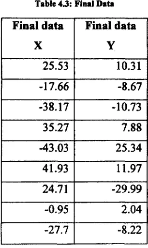
Table 4J: Final Data
Final data
X
Final data
Y
25.53 10.31
-17.66 -8.67
-38.17 -10.73
35.27 7.88
-43.03 25.34
41.93 11.97
24.71 -29.99
-0.95 2.04
-27.7 -8.22
The final data shown in Table 4.3 is plotted in a graph as shown in Figure 4.4. The
eigenvectors are represented as black dots in Figure 4.4.
Final d«u pkx with B«cnvKtors u thtir Axes
• — >Bgamcton vj.vj
I Eigenvector 1
Eigenvector 2
The Eigenvectors form the axes for the final data as shown in Figure 4.4. Incase we have
more eigenvectors; we would have more than two axes. The axes of eigenvectors are
always perpendicular which makes it more efficient to express the data set.
Fundamentally we have transformed our data set so that it is expressed in terms of
patterns between them. The patterns are the lines that can efficiently describe the
relationship between the data.
Comparing the original dataset with the final data set, as shown in Figure 4.5,
Comparing original data with the final data
Original Data
10 2S 30 45 SO
X Axis
Final data plot with Eigenvectors as their Axes
+ — >Bgenvtctors vj,v2
{Eigenvector 1
Eigenvector 2
X
Figure 4.5: Comparison between Original Data and Final Data
We can see that representing the data set in terms of their eigenvectors can efficiently
describe the relationship between the elements in the dataset. It clearly describes the
elements that do not give us any indication about the relationship between the elements.
This type of data analysis technique from PCA is used in eigenfaces method to classify
the image vectors.
4.5 PCA in Face Recognition
PCA is a statistical dimensionality reduction tool, Kirby and Sirovich (1990) [Kirb 87]
applied PCA for representing faces, Turk and Pentland (1991) [Pent 91] extended PCA to
recognize faces. To understand the role of PCA in face recognition, we should first
consider the representation of images.
Images are represented as a matrix of pixels. Consider an image of dimension
N x N\ this can be represented as N2 dimensional vectors by concatenating all the rows
into a single column. Similarly for 5 different images, each of dimension N x N, we will
have 5 different image vectors. Then we concatenate all these vectors together to get a
matrix. We then apply PCA on this matrix, which gives us the original data in terms of
eigenvectors. Once we get the test image, we project the test image on the image space.
Then we find the difference between the test image and the images in the database using
a distance classifier. This effectively discriminates the images in the database that
resemble the test image. Figure 4.6 illustrates the role of PCA and distance classifier in
Training Pha»« Twt Phaw Database of Training Image*
[*v*2.i3...jg
'*1' *2* *3— *r>!
[yi.y2.V3-Vn) lXl.K2.*3-*nI
Distance:**
: i*1« *2* *3"* *n»
Eigenfaces are obtained after scaflng ami projecting Eigenvector*
Feature \fector of "tart knag*
RESULT
Best Match tor Teat Image la Image 2
(with leaat distance between the feature vectors)
Figure 4.6: PCA in Face Recognition
PC A is a statistical analysis tool. To personalize PCA for face recognition, we need a
new algorithm. The EA developed by Turk and Pentland [Turk 91] [Pent 91] is one such
algorithm.
4.6 Eigenfaces
An Input image consists of many characteristic features. PCA is a mathematical tool that
we use to highlight and differentiate these features. Once we have these features for a set
of images, we find their feature vectors or eigenvectors. These eigenvectors are also
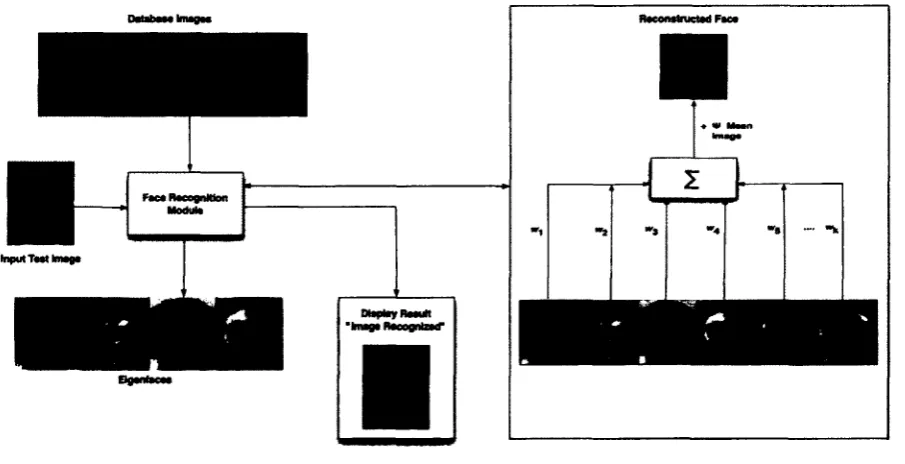
Once we have a set of eigenfaces for the database of images, we find the weights
that are required for the eigenfaces to reconstruct each image in the database. When we
are presented with a test image, we find the weight vector of the test face by projecting it
into the eigenfaces. We then compare the weight of the test face with the weight of the
images in the database using a distance classifier. This tells us how closely each
particular image in the database resembles the test image. This procedure is an extension
of PC A called as eigenfaces.
Sirovich and Kirby's efficient representation of faces using PC A was the
motivation for the concept of eigenfaces. Turk and Pentland extended PCA and arrived at
a method "that would build up the characteristic features by experience over time and
recognize a particular face by comparing the feature weights needed to (approximately)
reconstruct them with the weights associated with the known individuals" [Turk 91] [Pent
91].
With EA the individual images could be represented compactly as eigenfaces
based on their features. From these eigenfaces we can also reconstruct an image from the
database, since all we need are only the eigenfaces and since it is very compact,
eigenfaces would use very less memory.
Since the publication of eigenfaces many new algorithms have been proposed.
4.7 Eigenface Approach
The steps used in EA [Turk 91] [Pent 91] [Triv 09] [Carm 09] for face recognition are as
follows:
1. Initialization - The Images that constitute the database are assimilated
2. Calculation - The eigenfaces are calculated from the images in the database. The
M eigenvectors that correspond to the highest eigenvalues are kept. They
constitute the face space, and this is constantly updated as we obtain more images
for the database.
3. Finding Weights - The weight vectors of the known images are found by
projecting them into the face space. These weight vectors can be used to
reconstruct a face in the database using the eigenfaces.
The process mentioned above is done offline (back end process); we are required to
calculate the weights only when the database needs to be updated. The following are the
steps for recognition process; they used to be done online (front end process) whenever
the test image is produced.
1. When the test image is produced for identification, the weight vectors associated
with the test image are found by projecting them on the face space.
2. Once we have the weight vector of the test image, we compare it with the weight
vectors of the known images in the database, so that we can ascertain whether the
test face is a known face or an unknown face.
3. If the weight vector lies with in the face space, we can conclude that the given
Once we find the closest neighbor and if it satisfies the threshold condition, we
can say that the face is a know face from the database and its identity can be
established.
4. The eigenfaces and weight pattern are updated once we get new images for the
database. If there is an unknown face that is seen constantly, it could be labeled as
a known face and added to the database.