Computer-aided nonlinear modelling of continuous near-Markov processes.

University of Windsor University of Windsor

Scholarship at UWindsor

Scholarship at UWindsor

Electronic Theses and Dissertations Theses, Dissertations, and Major Papers

6-1-1971

Computer-aided nonlinear modelling of continuous near-Markov

Computer-aided nonlinear modelling of continuous near-Markov

processes.

processes.

Gary Arlo Tench University of Windsor

Follow this and additional works at: https://scholar.uwindsor.ca/etd

Recommended Citation Recommended Citation

Tench, Gary Arlo, "Computer-aided nonlinear modelling of continuous near-Markov processes." (1971). Electronic Theses and Dissertations. 6701.

https://scholar.uwindsor.ca/etd/6701

COMPUTER-AIDED NONLINEAR MODELLING OF CONTINUOUS NEAR-MARKOV PROCESSES

by

GARY ARLO TENCH

A thesis submitted in partial fulfilment of the requirements for the degree of

MASTER OF APPLIED SCIENCE

at the

UNIVERSITY OF WINDSOR

Department of Electrical Engineering Windsor, Ontario

UMI Number: EC53110

INFORMATION TO USERS

The quality of this reproduction is dependent upon the quality of the copy

submitted. Broken or indistinct print, colored or poor quality illustrations and

photographs, print bleed-through, substandard margins, and improper

alignment can adversely affect reproduction.

In the unlikely event that the author did not send a complete manuscript

and there are missing pages, these will be noted. Also, if unauthorized

copyright material had to be removed, a note will indicate the deletion.

®

UMI

UMI Microform EC53110

Copyright 2009 by ProQuest LLC.

All rights reserved. This microform edition is protected against

unauthorized copying under Title 17, United States Code.

ProQuest LLC

789 E. Eisenhower Parkway PO Box 1346

ABSTRACT

The implementation of a computer-aided

modelling technique is considered for continuous stationary ergodic near-Markov physical processes encountered in

practice. A procedure is given for the generation of a near- Markov process on an analogue computer. This process results

from the solution of an ordinary differential equation derived from a stochastic.differential equation defined in the sense of Ito. The stochastic differential equation describes a diffusion process to which the solution is a Markov process.

Methods for estimating the autocorrelation function and conditional incremental statistics of a near-Markov

process are illustrated. The conditional incremental statistics associated with a physical near-Markov process are analagous to the conditional incremental moment functions associated with a diffusion process. The statistical quantiti of a near-Markov process are of such a nature that a digital computer is required to compute their estimates from

sampled-data information.

For engineering ease of utilization the physical model takes the form of an ordinary differential equation. The modelling technique is illustrated for a specific near- Markov process generated on an analogue computer. This modelling technique has applications in the areas of simulation, filtering and identification.

ACKNOWLEDGEMENTS

The author would like to express his sincere gratitude to his supervisor Dr. W.C. Miller for his

guidance and continued inspiration throughout the course of the research.

The author is indebted to the National Research Council of Canada for financial support of the research in the form of a scholarship.

TABLE OF CONTENTS

Ppge

ABSTRACT i i

ACKNOWLEDGEMENTS iii

LIST OF FIGURES vi

CHAPTER 1 INTRODUCTION 1

.1.1 ' Random Processes in Engineering 1

1.2 Continuous Markov Processes 3

1.3 Diffusion Processes and Physical Models 3

1.4 Purpose and Contents 5

CHAPTER 2 ITO'S STOCHASTIC DIFFERENTIAL EQUATION 7

2.1 Introduction - 7

2.2 Stochastic Processes 7

, 2.3 Markov Processes 8

2.4 Processes with Independant Increments 9 2.5 Ito's Stochastic Differential Equation 10

2.6 Summary 13

CHAPTER 3 NEAR-MARKOV PROCESSES 14

3.1 Introduction 14

3.2 Ordinary and Stochastic Differential Equations 15 3.3 The Estimation of a Physical Model 18 CHAPTER 4 A COMPUTER-AIDED MODELLING TECHNIQUE 20

4.1 Introduction 20

4.2 Formation of the Near-Markov Process 21 4.3 Generation of the Near-Markov Process 26 4.4 Estimation of the Process Statistics 38

4.5 The Modelling Procedure 50

4.6 Summary 53

CHAPTER 5 CONCLUSIONS 55

REFERENCES 58

APPENDIX A - PAPER TAPE CODE CONVERSION PROGRAM 59 APPENDIX B - AUTOCORRELATION FUNCTION, PROBABILITY DENSITY

FUNCTION, CONDITIONAL FIRST- ’AND SECOND-ORDER

INCREMENTAL STATISTICS PROGRAM 63

APPENDIX C - ‘DISCRETE FOURIER TRANSFORM PROGRAM APPENDIX D - CALCOMP PLOTTING PROGRAM

LIST OF FIGURES Figure 4-1 4-2 4-3 4-4 4-5 4-6 4-7 4-8 4-9 4-10 4-11 4-12 4-13 4-14 4-15 Page The Scaled Analogue Computer Diagram used to

Generate the Near-Markov Process, V^(t) 24 The Block Diagram of the Experimental Apparatus used in the Generation of the (t) Process and in the Calculation of the Process Statistics 25 The Estimate of the Probability Density Function

of the Noise Generator's Attenuated Output,

•l z (t ) 28

The Estimate of the Autocorrelation Function of the Noise Generator's Attenuated Output, .lz(t) 31 The Estimate of the Power Spectrum of the Noise Generator's Attenuated Output, .lz(t) 34 The Estimate of the Autocorrelation Function of

the V^(t) Process 36

The Estimate of the Power Spectrum of the V^(t)

Process 37

The Sampling Procedure used for the Estimation of the Conditional Incremental Statistics of

the v ^(t) Process 40

The Estimate of the Probability Density Function

of the V^(t) Process' 41

The Estimate of the Conditional First-Order

Incremental Statistic of the V^(t) Process 43 The Estimate of the Conditional Second-Order

Incremental Statistic of the V^(t) Process 45 Photographs Taken from an Oscilloscope Connected to the AXO8-Laboratory Peripheral. Various

Statistics of the (t) Process and the Noise

Generator are shown 46 & 47

The Fitted Polynomial Approximation for the

Estimate of K p(v p) 48

The Fitted Polynomial Approximation for the

Estimate of K^(V^) 49

The Fitted Polynomial Approximation to P(U^) Computed from the Estimates of the K.(V,) and

K 0 (V^) functions 51

4 - 1 6 The Pitted Polynomial Approximation to Q(U,) Computed from the Estimates of the K,(V,) and K2 (Vx) functions

CHAPTER 1 INTRODUCTION

^ Random Processes in Engineering

Many systems encountered in engineering practice are random in nature. Examples of these are such items as flow meter outputs and noise corrupted communications

signals. In dealing with signals of this nature, it is necessary to utilize the theory of stochastic processes.

Miller (1969) gives the following definition of a stochastic process. A stochastic process is a math­ ematical abstraction of a physical phenomenon whose

development proceeds according to probabilistic laws. The theory of stochastic processes is related to that part of probability theory which deals with the interdependence and limiting behaviour of random variables. In many cases, the complex nature of the proofs for basic theorems relating to stochastic processes makes the transition from a math­ ematical abstraction to a useful engineering technique difficult.

be related to a special type of stochastic process called a diffusion process. This relationship and the contents of this thesis are easier to understand if the classification of

random processes is first considered.

A continuous random process may be classified according to the order of the probability density function necessary to characterize it. For a purely random process, all the information about the process is contained in the first-order probability density function. This is the simplest kind of random process. Unfortunately, a purely random process can only be considered as the limiting case of any continuous random process. A purely random process, frequently called white noise, has uncorrelated samples no matter how small the sampling interval is made. Any

process encountered in practice will have correlated samples if the sampling interval is made small enough.

The next more complicated random process has all the information necessary to characterize it in a

statistical sense contained in the second-order probability density function. A process having this characteristic

is the Markov process named after the mathematician A.A. Markov Other random processes characterized by higher order probability density functions exist but due to their math­ ematical complexity they are beyond the scope of this thesis.

pianatory; therefore, not too much difficulty should be encountered.

1.2 Continuous Markov Processes

Gaussian white noise plays an important role in explaining the properties of a certain class of continuous Markov processes called diffusion processes. Kolmogorov in

1931 has derived two important equations relating the con­ ditional probability density function of a diffusion process to the incremental moment functions of the process.

His second equation is commonly called the Fokker- Plank equation.

Diffusion processes are defined by stochastic differential equations. One precise definition of such an equation has been given by Ito (1951). The scalar form of his equation for a stationary diffusion process is written as

dx = f(x)dt + g(x)dy (1.1)

where y(t) is a Wiener process. It is important to note that equation (1.1) cannot be solved by the ordinary rules of

calculus. One advantage of equation (1.1) is that there is a simple relationship between it and the corresponding .

Fokker-Plank equation.

To solve equation (1.1), techniques such as those used by Stratonovich (1966, 1968) must be employed.

1.3 Diffusion Processes and Physical Models

4.

Most physical processes have a definite smoothness? whereas,

diffusion processes are not even differentiable. Thus, physical processes are at best near-Markov. Miller (1969) points out that if the noise source associated with the

random physical process has a short correlation time relative to the system, the physical process may possibly be near- Markov and hence can be modelled by a diffusion process. The exact ratio of correlation times necessary is dependant upon the particular system.

Stochastic differential equations cannot be solved using ordinary calculus techniques; however, it is often desirable to implement the modelled process as an analogue computer. This situation could arise if a new filter were being designed for a particular process. The modelled process could be generated on the analogue computer and used on-line to investigate the effects of various parameter changes in the filter. However, in order for the modelled process to be

generated on the analogue computer, the model must take the form on an ordinary differential equation.

Processes defined by stochastic and ordinary

differential equations can be related by computing their in­ cremental statistics. The incremental moment functions for a diffusion process can be estimated when the time interval

the process is sufficiently higher than the highest frequency component of the process. This criterion insures that the

physical process has sufficient Markovian properties to justify the diffusion model approximation.

The ordinary differential equation which corresponds to Ito's stochastic differential equation (1.1) is given in

equation (1.2)

™ = F (X) + G (X) z (t) (1.2)

at

z(t) is a physically realizeable Gaussian dis­

tributed noise source with a short correlation time, compared to that of X(t), and with an intensity coefficient of unity.

The functions g(x) and f(x) in equation (1.1) can be related to the incremental moment functions of the x(t) process. Similarilv in equation (1.2), G(X.) and F (X) can be related to the incremental statistics of the X(t) process. The incremental properties of the x(t) and X(t) processes can be equated to

determine the relationship between the functions in equations (1.1) and (1.2). This technique enables one to determine the appropriate diffusion model of the ordinary differential equa­ tion (1.2) or vice versa.

1.4 Purpose and Contents

In a practical situation equation (1.2) would not be known^and as stated in section 1.3, it is of greater engineering interest to have a model in terms of an ordinary differential equation.

for a near-Markov process. This is detailed in Chapter 3. He successfully demonstrated the modelling technique for three examples of near-Markov processes generated on a digital com­ puter. Using'Miller's (1969) modelling technique, the work in this thesis shows that it is possible to formulate a model for a physically realizeable continuous stationary ergodic near- Markov process based on sampled-data information. This is an

attempt to more nearly simulate an actual application of the modelling technique to a physical process.

The process is generated by solving a specific ordinary differential equation on an analogue computer. This equation has the same form as equation (1.2). Sampled data is taken from the process and a model based on first-order ordinary differential equation is formed. This model is again of the same form as equation (1.2).

Chapter 2 contains a discussion of Ito's stochastic differential equation as this is essential to the modelling technique.

Chapter 3 outlines the modelling technique itself while Chapter 4 gives the results of a model formulated for the near-Markov process generated on the analogue computer.

CHAPTER 2

ITO’S STOCHASTIC DIFFERENTIAL EQUATION

2.1 Introduction

This chapter is concerned with tthe concepts of

stochastic and Markovian processes. It deals with a stochastic differential equation, defined by the mathematician Ito (1951), to which the solution is a continuous Markov process. The incremental moment functions are developed for the process

defined by Ito's stochastic differential equation. Kolmogorov's foreward and backward equations are then given to show the

relationship between the incremental moment functions and the conditional probability density function of the process.

Processes with independant increments are discussed since they are basic to the understanding of Ito's stochastic differential equation.

2.2 Stochastic Processes

A stochastic process can be defined in the following manner as given by Gendenko (1966).

Let U be the set of elementary events and t a con­ tinuous parameter. The function of two arguments

<f(t) = 0 (e , t) (e C U) (2.

is called a stochastic process.

event), 0(e,t) depends only on t and is thus an ordinary

function of one real variable. Each such realization is called a realization of the stochastic process <£(t). If both e and t are variables, £(t) forms a collection of realizations and if e and t are both fixed £(t) is a single number.

A random process may be interpreted either as a

collection of random variables £(t) depending on the parameter t or as a collection of realizations of the process £(t). In order to define a process it is necessary to assign a probability measure in the function space of its realizations.

2.3 Markov Processes

A continuous Markov process is a special type of stochastic process and is often called a process without aftereffect. According to Papoulis (1965) , a process is Markovian in nature, in a loose sense, if the past has no in­

fluence on the statistics of, the future under the condition that the present is known. This can be stated in terms of conditional probabilities. For any n and t^ > t^ .... > t , the condition Pjx(t, ) < x, lx(t„) = x„ x(t ) = x } = Pj x(t,)<

* 1 1 2 2 n n ’ ' 1

XjJx(t2 ) = X2 l' is true for a Markovian processes. Their statis­ tics are completely determined if one knows merely their second- order probability density function.

2.4 Processes with Tndependant Increments

An explanation of processes with independant incre­ ments as adapted from Miller (1969) is given in this section.

If y(t) is a process with independant increments and y (t^) , Y (t2) , . . . y (tn ) ; t^< < . . . (n > 3) are realiza-tions of the process at times t.., , , ... t , the differences

c 1 2 n

[y(t2 ) - y (t 1 > ], [y(t3 ) - y ( t 2 )], ..., [y(tn ) - y ( t n _ 1 )] (2.2)

are m u tually independant. If the di s t r ibution y (t+At) - y(t) depends only on At, a process with independant increments is said to have stationary increments also.

Since processes with independant increments are specified by the distribution of the increments, the random variable of the process of interest is really y (t ) -

To avoid this situation, y(o) is defined as zero with probability one.

The Browian motion process has independant increments and properties that y (t+At) - y(t) is real and normally dis1- tributed with

E{y (t+At) - y(t)} s 0

E{[y (t+At) - y (t)]2 \ = a 21Atl (2.3)

where a 2 is the variance parameter. E { \ indicates the expectation of the quantities enclosed in brackets.

When the variance parameter of the Browian motion process equals one, the process is often referred to as a Wiener process. The Wiener process is especially important

Ito (1951). its solution is a continuous Markov process.

Another feature of the Browian motion process is that it is not differentiable. That is, dy(t)/dt cannot be finite for as Doob (1942) pointed out, since the variance of the

increments is proportional to t, the standard deviation is

I'

of the order (At) 2 . This results in equation (2.4).

y(t+At) - y ( t ) ~ (At)% (2.4)

This result is also important in the discussion of Ito's stochastic differential equation occurring in the next section.

2.5 Ito's Stochastic Differential Equation

Ito has formulated a stochastic differential equation which defines a continuous Markov process. The scalar form of this equation is given by equation (2.5)

dx (t) = f[x(t), t] dt + g[x (t) , t]dy(t) (2.5) where y(t) is a Wiener process with the following properties.

E{y(t2 ) - y (t1)| = 0

(2.6)

E i[y(t2 ) “ 55 Jt2 “ t l l

It is tempting to try to solve equation (2.5) by dividing-through by d t ‘and using conventional calculus tech­ niques; however, as shown in the previous section dy(t)/dt is not finite. Equation (2.5) can be solved by defining a special

7

Since the solution to equation (2.5) is a continuous Markov process, for certain conditions imposed upon the functions

f(x(t),t) and g(x(t),t), it is of interest to solve for the in­ cremental properties of the process defined by equation (2.5). The incremental moment functions of x(t) may be determined by taking the expectations of both sides of equation (2.5) then

dividing by At and taking the limit as At approaches zero. Performing these operations gives

E{x(t+At)~ x(t) f = E{f [x(t) ,t]dtf

+ g[x(t),t] E{y (t+At) - y(t)| (2.

£ M |x(t) = < } - f[Ct] . (2.6

Equation (2.8) is evident in light of equation (2.4). Squaring dx(t) and performing the same operations as in equation (2.7) gives

E{dx2 (t)| = E {(f [x (t) ,t]dt) 2 + 2 (f [x (t) ,t]dt) (g[x (t) , t]dy (t)

+ g2[x(t),t] [dy (t)] 2 }

lim p ([x(t+At) - x(t)]2 , ... _ l

At->0 5t lxit'

~ ^

= Ati

o

- g2K , h

(2.io

The conditional first- and second- order incremental moment functions are' defined by equation" (2.8) and (2.10) respec­ tively. The i-th order conditional incremental moment function of the x(t) process is defined by

For the x(t) process defined by Ito's stochastic differ­ ential equation.

_ . k^(x,t) = 0; i > 3 (2.12) as is true for a continuous Markov process or diffusion process.

Kolmogorov's equations (2.13) and (2.14) give a

relationship between the conditional probability density and in­ cremental moment function of a continuous Markov process.

dp (x,t I x ,t ) d p (x,tlx ,t ) --- 5 t T ^ = - f (x0 , tQ ) ---

gj---g2(xo ,to ) d2p(x,tlx0 ,tQ ) * 2

ox

(2.13)

d p ( x , t lx ,t ) . ...

---5t--- " = " 3 x

(Xrt^

2

[g2 (x,t) p (x, 11 x , t )] (2.14)

* d x 0

The second Kolmogorov equation is also known as the

Fokker-Plank equation after the physicists who first developed it. The conditional probability density function is shown in equation

(2.15).

p(x,x ;tft )

p(x,tlx ,t ) = 7----7— --- /O 1 C \

o' o p(xQ ,to ) (2.15)

In a steady state condition, that is, as t-t approaches infinity, the occurance at t is essentially independant of the

occurance at t Q and equation (2.1) reduces to

lim p(x,tlx ,t ) — p(x,t) (2.16)

which is the first-order probability density function and is usually of more interest.

2.6 Summary‘

Ito has defined a stochastic differential equation whose solution is a continuous Markov process. The solution to this equation is not obtainable using ordinary calculus techniques.

The incremental moment functions for the process defined by Ito's stochastic differential equation are developed and their relationship to the conditional probability density function is given in Kolmogrov's foreward and backward equations.

When a physically relaizeable process with near-Markov properties is considered, one is concerned with the infinitesimal properties of equations (2.17), (2.18) and (2.19) rather than the

incremental moment functions of equation (2.8) and (2.10).

E {x (t+At) - x (t) j x (t)| = f (x (t) , t)At + r?( At) (2.17)

E { [x (t+At) - x (t) ] ^ Ix (t)} = g^ (x (t) , t ) A t + rf(

At)

E {[x (t + A t ) - x ( t ) ] n |x(t)f = rj(At) (2.19) The reason for this will be discussed in Chapter 3 where the

relationship between Ito's stochastic differential equation

CHAPTER 3

NEAR-MARKOV PROCESSES 3.1 Introduction

If for a given continuous Markov process the incremental moment functions are known, then the defining stochastic differential equation, in the sense of Ito, may be deduced. These incremental moment functions are exactly specified by equations (2.8) and (2.10) when the evaluating time interval approaches zero. For a finite time interval, the incremental moments may be approximated by utilizing equations (2.17) and (2.18).

Since physical processes encountered in nature are at most near-Markov, their incremental properties only approximate those of diffusion processes.

It is possible to estimate quantities analagous to the incremental moment functions of a diffusion process from sampled-data information taken over a finite sampling interval from a near-Markov process. These quantities are referred to as the conditional incremental statistics. For a physical process, there will be a range.of sampling

intervals over which these incremental statistics can be evaluated and still be of a useful accuracy.

O n c e these conditional incremental statistics have been computed, the stochastic differential equation, in

15.

In Engineering work, diffusion processes are usually only of academic interest. Since it is often

desireable to model the process on an analogue computer, it is necessary to obtain an ordinary differential equation whose solution is a near-Markov process with statistical properties similar to the near-Markov process being modelled. In order to estimate the specific functions appearing in the ordinary differential equation chosen as the model, it is

necessary to relate the estimates of the incremental properties of the process to those functions.

3.2 Ordinary and Stochastic Differential Equations

This thesis is concerned with modelling a continuous stationary ergodic near-Markov process with a first-order ordinary differential equation of specified form. First

however, the relationship between an ordinary and a stochastic differential equation will be considered.

One might be tempted to formulate an ordinary differential equation by dividing through in equation (2.5) by dt and replacing dy(t)/dt by a realizeable Gaussian band-limited noise source z (t). This result is shown in equation (3.1).

shown that as z(t) approaches white Gaussian noise, in general, the solution to equation (3.1) does not converge to that of the diffusion process defined by Ito's stochastic differential equation.

The relationship between the stochastic and ordinary differential equation is much more complex. Consider the

first-order ordinary differential equation given in equation (3.2).

= F(X) + G (X) z (t) (3.2)

X(t) is a near-Markov process and z(t) is a stationary Gaussian distributed noise source with zero mean value and having a

very short correlation time. The correlation time of the noise and the intensity coefficient, which is equal to unity in equation 3.2, are defined by equations (3.4) and (3.5) respectively. Both equations involve the autocorrelation function of the noise. This is given in equation 3.3 for a stationary ergodic noise source.

T

0

= E{z(t+r) z(t)} (3.3)

00

■ 'o o r (2) = 3t / IBzZ (r)ldri = R Z Z (0) < M )

Vo.

+ 00

O.-(a) =

f

1

J zz

— oo

17.

Kx (X) w F (X) + j G(X) ( 3 . 6 )

K2( X ) « g2( x ) (3.7)

These equations are only valid if Ch (z) is equal to unity. K^(X) and K 2 (X), computed from an ordinary differential equation, are functions analagous to the incremental moment functions of a diffusion process and are called the conditional incremental statistics.

The form of the stochastic differential equation, in the sense of Ito, that defines a diffusion process with corresponding incremental moment functions k-^(x) and ,k2 (x) is given in equation (3.10).

Stratonovich has thus been able to show the relationship between a stochastic and a first-order ordinary differential equation. He also gives the conditions under which the

s o lution to equation (3.10) has .statistical properties

sufficiently close to the near-Markov process to form a satisfactory model. A detailed treatise of this portion of Stratonovich's work is given by Miller (1969).

k^ (x) = F (x) + ~ G (x) (3.8)

k 2 (x) = G 2 (x) (3.9)

3.3 The Estimation of a Physical Model

The theory so far has dealt with finding the

appropriate diffusion model for a near-Markov process defined by a given ordinary differential equation. However, the

problem is to formulate a model in terms of a first-order ordinary differential equation based on estimates taken from a physical near-Markov process.

If a stationary near-Markov process is encountered that can be modelled by a first-order ordinary differential equation such as (3.2),

= p (X ) + G (X) z (t) (3.2)

then the results of section 3.2 are useful. The functions P(X) and G(X) can be computed from a knowledge of the conditional incremental statistics K. (X) and K„ (X). This

u. Z

can be shov?n by rearranging equations (3.6) and (3.7) as follows:

n (X)'

F (X) = K 1 (X) - f (3.11)

G (X) =

t

For these latter two equations to be valid, z (t) in equation (3.2) must have a small correlation time and a unity intensity coefficient. As pointed out by Miller (1969), the condition that the ratio of the upper frequency component of the noise source to that of the process generated by equation

(3.2) is large will also ensure that the solution to equation (3.2) is near-Markov.

differential equation (3.2), whose solution is a near-Markov process, may be formulated from a knowledge of the conditional incremental statistics, computed from sampled-data, and the use of equations (3.11) and (3.12). This model has the same statistical properties as the process itself but it is important to note that the terms of the ordinary differential equation have no correspondance to anything generating or involved with the process itself.

Once the correct form of equation (3.2) has been deduced, there appears to be no way to check its accuracy other than solving it on a computer and comparing its

statistical properties with those of the original process. This problem has been avoided in this thesis by solving an ordinary differential equation of the form given in equation (3.2) on an EAI 580 analogue computer. The process is sampled

and analogue-to-digital conversion is performed by an AX08- Laboratory Peripheral under control of a PDP-8/I digital computer. The estimates of the conditional, incremental statistics are computed, as outlined in Chapter 4, and estimates of the functions F(X) and G(X) are computed from equations (3.11) and(3.12). These functions are then

compared with those of the original equation implemented on the analogue computer in order to obtain an estimate of the

CHAPTER 4

A COMPUTER-AIDED MODELLING TECHNIQUE

4.1 Introduction

This chapter describes a computer-aided modelling technique for obtaining diffusion or1 physical models of

physical processes. A diffusion model is formulated using a stochastic differential equation whereas a physical model is formulated using an ordinary differential equation. In this thesis, a physical process is considered a process for which a satisfactory stationary diffusion model based on a scalar stoch­ astic differential equation of the type defined by Ito can be formulated. For a suitable diffusion model to be found,

the physical process must be near-Markov in nature.

The statistical properties of a Markov diffusion

process are defined by the incremental, moment functions. These are defined as the time increment approaches zero.

No physical process encountered in practice is strictly Markov; therefore, the incremental properties do not exactly

characterize it. However, if the process is sufficiently near- Markov, its analogous incremental properties can be evaluated using a non-zero time interval. These properties are referred to as the conditional incremental statistics of the process.

In order to evaluate the conditional incremental

with a short correlation time, then the smallest sampling interval, according to Miller (1969), should not be less than the .correlation time of the noise source. As can be seen from equations (2.17), (2.18) and (2.19), the larger At is the

larger the error. An upper bound on At is set by the process correlation time. The optimum sampling interval,At, lies some­ where between the noise and process correlation times as given in equation (4.1),.

rd o r ^ ^ < rcor^V l^ (4.1)

In order to verify the modelling procedure introduced in Chapter 3, a continuous near-Markov process is generated on an analogue computer. This is done by solving a given first- order ordinary differential equation whose driving function is a random noise source. A physical model is then formulated based on sampled-data information obtained from the process. The form of this model is a first-order ordinary differential equation of the same form as the equation used to generate the process. The accuracy of the model is then checked by comparing corresponding functions in the two equations.

4.2 Formation of the Near-Markov Process

The first step in the modelling procedure is to generate a continuous near-Markov process. T h e •first-order ordinary

differential equation implemented on the analogue computer to generate the near-Markov process is derived from work done by Astrom (1965) on the scalar stochastic differential equation

(4.2) defined in the sense of Ito.

The corresponding Kolmogorov equations are:

ap(Tj_,t(v ,t ) ap(v1,tlvo ,to) 2 a2p(vl'tlvo'to ) ,, ,, --- ~ x --- ^--- _ (1+V )---7j v 4 . J J

o ° dvo 1 dvc2

dp(v ,tlv , t ) v , s2 ~

= _ (-vl)p(v1,t.!vo ,to) + 2 — 2 2(l+v1) p(vr tlvo ,tc

i dv^

. (4.4)

The steady state solution of equation (4.4) .for the probability density function is:

O

lim p(v1 ,tl v0 ,tQ ) = w(v1) = (l+v1) exp[-l/(l+v1)] t~t— ^►00

0

(4.5) As can be seen from equation (4.2), the incremental

moment functions of the process are given by:

kl^Vl^ = -V1 (4.6)

k2 (vl} = 2(vi+ 1 ^2 (4 ‘? )

Us ing equations (3.10) and (3.11) and setting (V^)

kf (Vf) and ^ ( V ^ ) = ^2^V 1^ one °ktains ^ le functions.

F(V1) = -2V1-1 (4.8)

G ^ ) = V 2 -’(V1+1) (4.9)

Thus the ordinary differential equation whose solution is a continuous near-Markov process with statistical properties similar to those of the diffusion process defined by equation

(4 . 2) is dV^ (t)

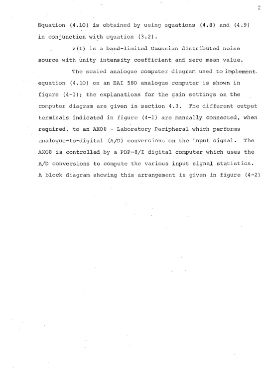
Equation (4.10) is obtained by using equations (4.8) and (4.9) in conjunction with equation (3.2).

z(t) is a band-limited Gaussian distributed noise source with unity intensity coefficient and zero mean value.

The scaled analogue computer diagram used to implement- equation (4.10) on an EAI 580 analogue computer is shown in

figure (4-1); the explanations for the gain settings on the

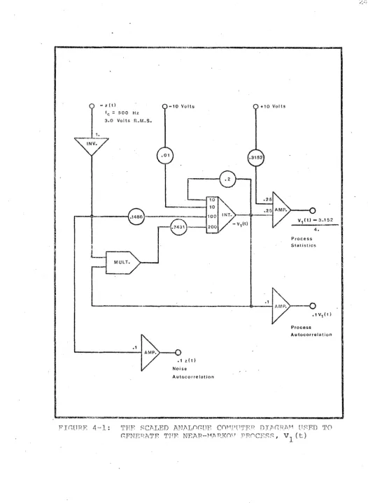
computer diagram are given in section 4.3. The different output terminals indicated in figure (4-1) are manually connected, when required, to an AX08 - Laboratory Peripheral which performs

f q = 5 0 0 H z 3 . 0 V o l t s F i . M . S ,

I N V .

. 3 1 5 2

2 5

A M P . . 2 5

1 0 0

. 1 4 8 6

200

1 . 7 4 3 1 1~

P r o c e s s S t a t i s t i c s

M U L T

— o AMP.

Process

A u t o c o r r e l a t i o n

A M P .

N o i s e

A u t o c o r r e l a t i o n

W |.r i|iill i iinwri'Mh'uifimiiii iiij.i i iii11rin i iiiiiT tn rn nBr w m m ru m n i ru m m ~ in n ~ m m riin w n i[iim u iiim m n iiirJ L iriirT irT

P U N C H / R E A D E R .

T E L E T Y P E N O I S E

GE NE R AT OR

OSCILLOSCOPE DI SPLAY

A X 0 8 -L A B O R A T O R Y P E R I P H E R A L

P D P - 8 / 1 D I G I T A L C O M P U T E R E A I 5 8 0

A N A L O G U E C O M P U T E R

4.3 Generation of the Near-Markov Process

Equation (4.10), whose solution is a continuous

near-Markov process, is not as easily implemented on the analogue computer as one might at first think. Problems occur because of the random nature of the process and because the random driving function, z (t), in equation (4.10) has to have certain specific characteristics. Measurements must be made on z(t)

to ensure that correlation time, bandwidth and probability density function requirements are met. Measurements are also necessary to determine the proper analogue potentiometer and amplifier gain settings to ensure that the noise source has an effective unity, intensity coefficient.

The noise generator, designated -z (t) in figure (4-1), had its gain adjusted to produce an output signal of 3.0 volts R.M.S. with zero offset voltage. From sampled-data information taken at the point in figure (4-1) labelled .lz(t), the noise probability density and autocorrelation functions can be

computed. -z (t) is attenuated before.sampling occurs because of the voltage restrictions on the A/D converters in the AX08.

Since the exact attenuation factor is known, .1, this can be accounted for in all calculations.

The exact method used to calculate the noise probability density function is given in section 4.4 when measurements of

assembler language PAL III is given in Appendix B. The changes necessary to the program to make it capable of

calculating the noise probability density function are indicated in the program.

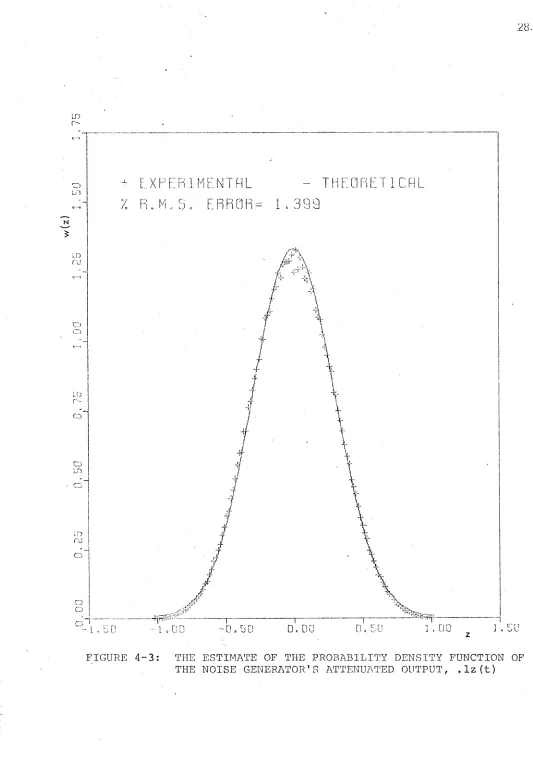
Figure (4-3) shows the estimated and theoretical, w(Vj), noise probability density functions. The estimated

noise probability density function was computed from sampled- data information obtained from the .lz(t) terminal in figure

(4-1). The R.M.S. error based on the difference between the plotted theoretical and estimated values and expressed as a percentage of the maximum theoretical value is 1.3 99 percent. All other error calculations performed in the thesis are

calculated in a. similar manner. These results indicate that the noise probability density function is reasonably Gaussian distributed with zero mean value as it should be.

Figure (4-3) was plotted using a Calcomp plotter connected to an IBM 360 Model 65 digital computer; however,

in order to achieve this end result a few intermediate steps were necessary.

The data for the experimental probability density

function, formulated from the sampled-data information, was avai­ lable on punched paper tape output by the PDP-8/I in ASCII

paper tape code. A computer program was then written for the

PDP-8/I which accepted paper tape with the ASCII code and punched out an output paper tape containing the same information but punched in an IBM code. This newly punched tape was then

28.

ID

r-L X P E n l M E N T H r-L

u

D. DC *J1.

0 0 r: '!

2y.

plotted on the Calcomp plotter by the IBM 360 using a plotting subroutine written in the language Fortran. This same procedure was -followed for most of the figures in the thesis. A copy of the Fortran plotting subroutine, as well as a copy of the, PAL III assembler language program which converts ASCII coded paper tape to IBM coded paper tape, is given in Appendices D and A

respectively.

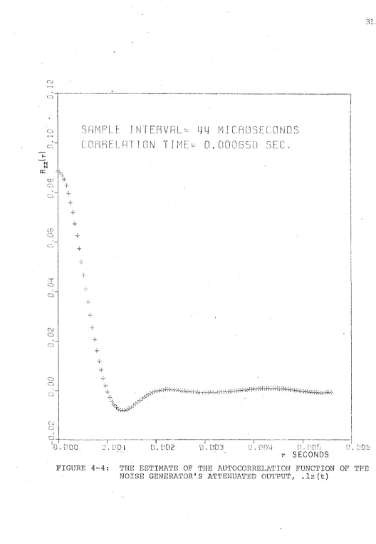
In order to obtain bandwidth, correlation time, and intensity coefficient measurements concerning the noise, it is necessary to estimate the autocorrelation function of the noise. For the stationary ergodic process, V^(t), autocorrelation is defined as in equation (4.11).

T

l'vi (t+r)V1 l

= E(vi (t+r)V1 (t)( (4.11)

Equation (4.11) can be implimented. on the digital computer for a finite record length using the formula given, in equation (4.12).

i N

Ry

y

1 1 n=o

At is the time between samples; N is the number of samples taken; and NAt is the record length.

labelled .lz(t) in figure (4-1). These are stored in successive core locations in the PDP-8/I computer. The first sample in the array is then successively multiplied by the contents of the same array and each product is added again successively to a second array of 12 8. The second array is initially set to zero and is used to accumulate the partial sums of the products

at the various delay times. The first array is used only as a buffer for each new array of 128 sampler.

To compute the estimate of the noise autocorrelation, the contents of the second array have only to be divided by the number of times an array of 12 8 samples has been taken. Figure^

(4-4) shows the noise autocorrelation estimate after 20,000 samples have been used to estimate each plotted point. This was considered a sufficient quantity to ensure an accurate

estimate of the autocorrelation function without causing any quantization error. A listing of the program written in PAL III assembler language used to calculate autocorrelation function

estimates is given in Appendix B. .

From the estimate of the autocorrelation function, other process properties are easily obtainable. For instance, the noise intensity coefficient can be obtained using equation

(4.13).

N

c. (z) = 2 V R (iAt)At; N = 128 _ r (4.13)

o

N N

( X

RLE I N T E R V A L

C O R R E L A T I O N TIN

44 M I C R O S E C

.0.000650 SEC

CD

n*

C\J

■4--n , hp

::■_}

----0. 0 00; 0 , D D L D. 00 2 CL DO 3 c l no3 n.nos

t S E C O N D S

n . ft nr

calculated. ‘This is given in equation (4.15)

az (t) a2R (r) ( 4 . 1 4 )

a

zz

1

(4.15)

In order to properly solve equation (4.10) an analogu computer diagram is first drawn assuming ~z (t) has the required intensity coefficient. The appropriate loop gains are then adjusted by 'a'. For the configuration given in figure (4-1), the noise source, -z(t), has a value of 3.0 volts R.M.S. and 'a has a value of 105.1. It is important to note in figure (4-1) that most of the noise amplification is done at the integrator input. This means that the amplified noise signal is never formed explicitly and amplifier overloading is avoided. Final adjustments to the gain are made using the appropriate

potentiometers.

of a function switch on the noise generator. As indicated earlier in Chapter 3, it is desireable to have this cutoff frequency as high as possible; however, the main criterion is that the ratio of noise bandwidth to system bandwidth be high. Later this will be shown to be true^

next switch position of lKHz, the estimate of the noise intensity coefficient would be adversely effected. This is due to both hardware and software restrictions placed on the time for an A/D conversion. This results in not as many points being available on the non-zero position of the

The noise signal was band-limited to 500 Hz by means

autocorrelation function. Even with faster A/D conversion, higher amplifier gains would be required to obtain a unity noise intensity coefficient. The required gain was to appear at the integrator inputs and was unfortunately of such a

magnitude that it was necessary to increase all integrator inputs and not just those associated with the noise. To compensate for the undesired gain at certain terminals,

attenuating potentiometers must be included in series with these inputs. Only a limited amount of attenuation is possible before all accuracy is lost.

It is necessary to examine the spectral properties of the noise to ensure that it has a relatively large bandwidth compared to that of the process. A Fortran subroutine was

therefore "written to calculate the discrete Fourier transform (DFT) of sampled-data information. This DFT is based on the fast Fourier transform algorithm as discussed by Brigham and Morrow

(1967). A listing of the program as well as a short

description of the theory of the fast Fourier transform is given in Appendix C .

According to Papoulis (1965), the power spectrum of a process is given by the Fourier transform of its autocorrelation function. Thus, the noise power spectrum was estimated by

taking the DFT of the estimate of the noise autocorrelation functic This is shown plotted in figure (4-5). The magnitude is plotted in d& which was obtained by calculating twenty times the

M

A

G

N

IT

U

D

E

d

B

CD I

CO

Q'J

LJT

fn

o O

S P E C T R U M C R L C U L R T E D FROM DFT

GF N

I

F R UTGCGRRELflTIDN

+

0 0.0 PUO.n >4 G 0.0 BOD'. 0 OOCJ.O 1000,0 10

F R E Q U E N C Y Hz

obtained from the abscia value in figure (4-5) when the noise power spectrum magnitude was 3 dB less than the maximum value.

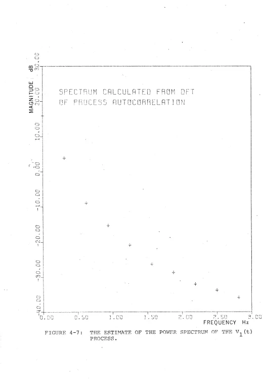
Ficjure (4-6) shows the estimate of the autocorrelation of the process, corrected for attenuation, as calculated from

sampled-data information taken from the terminal in figure (4-1) labelled .lV^(t). This is done in the same way as for the noise autocorrelation. The process power spectrum in figure (4-7) shows the bandwidth to be approximately 0.1 Hz. Thus, the ratio of noise to process bandwidth is 5,000.

The computational formula for the noise correlation time is given by equation (4.16); the process correlation time ' is calculated in the same manner.

N

rc o r (z) = F T o r X l R „ (iAt)|At (4*16)

zz

.r

0

Both the ratio of bandwidths and correlation times are large indicating that the noise is sufficient in this

respect to be used reliably in equation (4.10). Either of the ratios would have been sufficient since they give similar

information but both were computed as a cross-check. One is estimated from time domain information; whereas, the other is estimated using frequency domain information.

The measurement of the noise statistics is then

complete. The noise is shown to have the necessary properties as outlined in Chapter 3, to be used in equation (4.10) to generate the near-Markov process. All that remains is to

>_r—H >

£ X (

r\.i

O O

i.r.3

r--LD rj

O

S A M P L E I NTERVRL. =

HIL L I S E C O N D S

C O R R E L A T I O N T I M E -

SEC.

T._f

‘-r

t,,

•rn

'n:-p.

r-p__i

1

•'ivrr 0T( 5U 1r, 00 iT5o zToo /U 3

r S E C O N D S

F I G U R E 4 - 6 : T H E E S T I M A T E O F T H E A U T O C O R R E L A T I O N F U N C T I O N O F

MA

G

NI

TU

DE

;

d

B

0 * 7 O / .

V-J

O

O-ro

o O OJ

o 'O CD.

r ' ?? * *o

q "

o Q Q

O Q

O o o CO.

'—I

3 4.

S P E C T R U M C f l L C U L P i T E D F R O M D P T

GF P R G C E S S A U T O C O R R E L A T I O N

F R E Q U E N C Y Hz

4.4 Estimation of the Process Statistics

In order to construct a model for the V^(t)

process,

it is necessary to estimate the conditional incremental statistics of the process. The estimate of the conditional first-order incremental statistic, Kp(v q)f anc^ the estimate of the conditional second-order incremental statistic, K^CV^),- of the (t) process have been computed using the relationships given in equations (4.17) and (4.18).

. V. ( (n+1) A t ) - V (nAt) .

= E {— --- ^ ---- - IV'1 (nAt)| (4.17)

'[V,((n+l)At) - V ,(nAt)] 2

k 2 (Vx) = E i — --- 1---IV^CnAt)} (4.18)

These equations are basically equations (2.17) and (2.18) with the last terms omitted.

The estimates of these functions were computed from sampled-data information taken from the V-, (t) process using

the configuration shown in figure (4-2). Samples were taken from the terminal labelled (V^ (t)-3 .152)/4 in figure (4-1); this

scaling was done to accommodate the hardware limitations of the A/D converters in the AX08 and was accounted for in the program. • Three arrays of storage, each with 128 locations, were allocated for computation of the process statistics; these

arrays were initially set to contain all zeros. The range between the maximum and minimum values of V^(t) of interest is divided up into 128 equal intervals. Each of the 128 intervals is associated with one of the storage locations in each array. When the

which corresponds to this interval has its value increased by one.

A second sample is taken At seconds later and the

incremental change, ((n+1)At) ~ V^(nAt), is calculated. This added to the contents of the storage location in the second

array which is determined, as before, by the magnitude of V 1 (nAt) . The second array is used to sum the values of the incremental changes of the V^(t) process. This sampling procedure is shown graphically in figure (4-8). The time between successive increments, T, is determined by program

instruction time and is immaterial to the incremental calculations. The third array is used to sum the values of the square of the incremental changes. A s 'in the case of the second array, the appropriate storage location in the third array has its

value increased by [V^ ( (n+1)At - V^ (nAt)]^

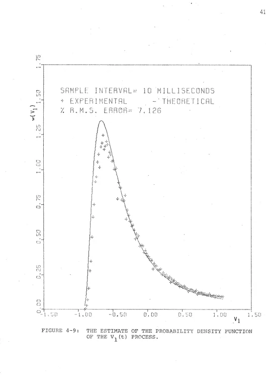
This procedure is continued until 1,000,000 samples have been taken. The magnitude of the probability density

function which corresponds to the mid-point value of the k-th interval is calculated by dividing the number contained in the storage location in the first array associated with the k-th increment by the product of 1,000,000 with the interval size. The estimate of the probability density function of the Vj(t) process is shown in figure (4-9) along with the theo­ retical probability density function, w(V^), for the corres­ ponding diffusion .process. There is a 7.126 percent R.M.S. error between the two.

For a suitably chosen At, the estimates of the

V-j( ( n + 1 ) A t ) - V ^ ( n A t )

rViC ( n + O ^ t + T ) - V-| ( n A t + T)

(n + l ) A t

nA t nAt + T (n + 1) A t + T

41.

Lf>

I''

-S A M P L E I N T E R V A L

+ E X P E R I M E N T A L

X R . M . S . E R R O R =

T H E O R E T I C A L

+jT'

Q

O

42.

of the incremental moment functions, k^(V^) and k^CV^), associated with the diffusion model for the (t) process. Based on a knowledge of the noise autocorrelation function and suggestions made by Miller (1969) concerning this process, At was chosen to be 10 milliseconds.

Using equation (4.17), the condition first-order incremental statistic, was estimated. This was done using the contents of the first two arrays. A plot of the estimate of (V^) along with the theoretical value of the conditional first-order incremental moment function, k^(V^), of the corresponding diffusion process is given in figure

(4-10). ^ ( V ^ ) ^as the f°rm given in equation (4.19).

kl (Vl} = ~V 1 (4.19)

Both functions are plotted over the range -0.912 to +1.104; this was considered adequate as 92 percent of the V^(nAt) values fell in this range.

The R.M.S. error between the estimate of k q_(v j_) and the theoretical value of k (V., ) is 31.9 percent. This

1

value at first appears quite large but is. in fact realistic when the probability density function of the (t) process is

examinedj The estimate of the function, K^(V^), in the range

-0.8 < V'1 (nAt)<0.5 is made using approximately 38.5 percent of the samples; however, in a similarly sized interval 0.7<V^(nAt) < 1.0 where the dispersion is high only 3.1 percent of the 1,000,000

samples were used in estimating K^(V^).

An estimate of the conditional second-order

in

o

> 1— !

r;j o ro

o o

OJ

c

o

o o o

c.:j

o

S A M P L E INTERVAL^

+ E X P E R I M E N T A L

X R.M.S.

ERR!

10 M I L L I S E C O N D S

- ' T H E O R E T I C A L

+

p T p

T.

T

+

1. . 00 -0. 5 0 oVoo D, 50 iVocT '1 FIGURE 4-10: THE ESTIMATE OF THE CONDITIONAL FIRST-ORDER

44.

and third arrays. A plot of the estimate of K 2^V 1^ al°n9 with the theoretical value of the conditional second-order

incremental moment function, ^2^V 1^' t'ie corresPon'^;*-n9 diffusion process is given in figure (4-11). k 2 (V^) has the form given in equation (4.20).

k 2 (V1 ) = 2(1+V1 )2 (4.20)

The R.M.S. error between the estimate of K^(V^) and the theoretical value of k2 (V^) is 3.571 percent. It is evident that the dispersion of the values for K 2 (V^) is quite small compared with the dispersion of the values of K^(V^). Miller (1969) found that this was always the case for the

»

discrete physical processes he investigated. The reason for this has not been successfully explained.

Photographs taken of the various process statistics are shown in figure (4-12). These photographs were taken from an oscilloscope connected to the display terminals of the AX0 8 as shoitfn in

figure (4-2).

45-o o

ZT T~H

C .j o C\J.

<NJ

zc

o o

o.

o

o o

o o

r.1J

O o

cj"

o o o

S A M P L E INTERVAL:

+ E X P E R I M E N T A L

X R „M .S . E R R O R

-10 M I L L I S E C O N D

• T H E O R E T I C A L

3, 571

- 1 , D 0

FIGURE 4-11

0. DC

r t\-n _'iH

FIGURE 4-12a:

SAMPLE OUTPUT FROM THE NOISE GENERATOR.

SCALES:

HOR. - 10.0 MILLISECONDS/CM VERT. - 0.2 VOLTS/CM

FIGURE 4-12b:

THE ESTIMATE OF THE PRO­ BABILITY DENSITY FUNCTION OF THE NOISE GENERATOR'S ATTENUATED OUTPUT, .lz(t). SCALES:

HOR. - 0.02/CM VERT. - 0.02/CM

FIGURE 4-12c:

THE ESTIMATE OF THE AUTO­ CORRELATION FUNCTION OF THE NOISE GENERATOR'S ATTENUATED OUTPUT, .lz(t). SCALES:

HOR. - 1.0 MILLISECOND/CM VERT. - 0.02/CM

FIGURE 4-12d:

THE ESTIMATE OF THE AUTO­ CORRELATION FUNCTION OF THE V,(t) PROCESS.

SCALES:

HOR. - 0.5 SECONDS/CM VERT. - 0.25/CM

FIGURE 4-12: PHOTOGRAPHS TAKEN FROM AN OSCILLOSCOPE CONNECTED TO THE AXO8-LABORATORY PERIPHERAL. VARIOUS

FIGURE 4-12e:

SAMPLE OUTPUT OF THE V,(t) PROCESS.

SCALES:

HOR. - 0,5 SECONDS/CM VERT. - 1.0 VOLT/CM

FIGURE 4-12f:

THE ESTIMATE OF THE PRO­ BABILITY DENSITY FUNCTION OF THE V.(t) PROCESS. SCALES:

HOR. - 0.25/CM VERT. - 0.2/CM

FIGURE 4-12g:

THE ESTIMATE OF THE C O N ­ DITIONAL FIRST-ORDER INCREMENTAL STATISTIC OF THE V,(t) PROCESS. SCALES:

HOR. - 0.25/CM VERT.- 0.5/CM

FIGURE 4-12h:

THE ESTIMATE OF THE CON­ DITIONAL SECOND-ORDER INCREMENTAL STATISTIC OF THE V.ft) PROCESS.

SCALES:

HOR. - 0.25/CM VERT. - 2.0/CM

M

V

i

)

O Cj

ro

-

F I T T E D

- . T H E O R E T I C f l i

% R « M . S . E R R O R - 1 4 . 3 2

rj_

T R E G R E T I C f l L

30Q

>

E R R O R

_ r

4.5 The Modelling Procedure

In order to smooth the estimates of K^ V 1^ anc^ K 2^V 2^' a standard least-squares curve fitting technique is used to ap­ proximate these statistics by a first and second-order polynomial respectively.

The polynomial approximations to K^(V^) and K 2 (V^) are shown in figures (4-13) and (4-14) respectively. The theoretical values of the incremental moment functions k^(V^)

and 1&2 (V^) are also plotted for comparison. The R.M.S. error

between K^(V^) and k^(V^) is 14.32 percent while between and k2^V l^ ^ 3,2 percent. The plotted polynomials for K f ^ f ) and K2 (V^) are given in equations (4.21) and (4.22).

K1 (V1 ) = °*138 ~ 0.907 V x (4.21)

k2 (Vi) - 1.82 + 3.72 V, + 1.92 V± 2 (4.22)

Using the conditional incremental statistics of

equations (4.21) and (4.22) and the relationships in equations (4.23) and (4.24) the model for the V-^ft) .process, the U ^ t ) process, can be formulated.

1 bK (U )

P(U1 ) = K1 (U1 ) - ~ — (4.23)

Q(UX ) = ± V k2 (U2r (4.24)

P(U1) = -0.792 -1.87U1 (4.25)

Q(U3 ) = V l . 8 2 + 3 .72U1 + 1.92U12 (4.26]

o Cj

rj

P- I T T E [J

ro

Q.

R « M , 5

-

T H E O R R T I C R !

R= 7 . 3 1 3

— r j (

----"0,'jC! D . C i O D . U U

'1 FIGURE 4-15: THE FITTED POLYNOMIAL APPROXIMATION TO P(U,)

Q

C

U

i

)

52,

o O

+ F i T ' l T l J '/

R . M . S .

F R f

T H F Q R F T I C R L

:i 319

[ip

u

The random forcing function r(t) has the properties outlined in Chapter 3 for z(t).

Equation (4.27) is identical in form to equation (4.10) which is used to generate the V^(t) process. Therefore, a

measure of the accuracy of the modelling technique can be assessed by a functional comparison of the experimental values of P and Q

from equation (4.27) and the original values of F and G used in equation (4.10).

These comparisons are shown in figures (4-15) and (4-16) respectively. The R.M.S. error between P and F is 7.31 percent while between Q and G it is 2.3 2 percent.

4.6 Summary

This chapter describes a computer-aided modelling technique whereby physical or diffusion models are estimated for near-Markov physical processes encountered in practice.. Problems associated with generating a near-Markov physical process on an analogue computer are discussed as well as those problems associated with the digital equipment involved. The

success of the modelling procedure can -be evaluated by determining how closely the model compares to the generated process. This is accomplished by comparing corresponding functions in the first-order ordinary differential equation used to generate the process and that used to model the process.

CHAPTER 5 CONCLUSIONS

Certain Markov processes can be precisely defined by a stochastic differential equation. Near-Markov physical process have been defined by a specific ordinary differential equation in­ volving the transformation of a realizeable noise source. Research has been primarely concerned with obtaining a diffusion model for a near-Markov physical process defined by a given ordinary dif­ ferential equation. This type of problem is associated with the relationship between ordinary and stochastic differential equations.

The incremental properties of a diffusion process can be related to the form of the stochastic differential equation de­ fining the process. Correspondingly, the incremental properties of a near-Markov physical process can be related, in an approximate fashion, to the form of the ordinary differential equation defining the process.

The statistical properties of a diffusion process are

exactly specified by the incremental moment functions of the process. For a sufficiently near-Markov physical process, functions anala- gous to the incremental moment functions can specify its statistics to a useful accuracy.

The incremental properties of a diffusion and a near-Markov

process can be equated to determine the r e l a t ionship between the

functions appearing in the corresponding stochastic and ordinary differential equations. This technique enables one to determine the appropriate diffusion model for a physical process defined by a given ordinary differential equation. When this technique in

conditional incremental statistics from sampled-data information allows both diffusion and physical models to be formulated.

This thesis has described the modelling procedure asso­ ciated with a continuous stationary ergodic near-Markov process. A model based on a first-order ordinary differential equation has been formulated using estimates of the incremental statistics of the process. These estimates have been computed by a digital com­ puter using on-line sampled-data information. The ordinary dif­

ferential equation of the model formulated was of the same form as that of the equation used to generate the near-Markov process on the analogue computer. In order to gain a measure of the accuracy of the modelling procedure, the corresponding functions in the two equations were compared. When the final estimates of F (V^) and G(V^) were computed, there was found to be a 7.3 and a 2.3 percent R.M.S. error respectively.

This thesis deals only with modelling techniques involving scalar near-Markov processes. More work needs to be done with

physical processes to determine if this is generally sufficient. The modelling technique could logically be extended to a multidimen­

sional near-Markov process but the mathematics becomes much more involved.

reason-able estimate based on those results■given in Chapter 4 and those given by Miller (1969).

To determine if a suitable sampling rate is being used requires a great deal of computation. The physical model must be formulated based on estimates taken from the process. The physical model must then be solved on either a digital or analogue computer

and measurements taken on its statistical properties. These statis­ tical properties are then compared to the statistical properties of the original process to obtain an indication of the accuracy of the model at the chosen sample interval.

There is another point which should also be mentioned.

It is possible that a process is ergodic with respect to some of its statistical properties and not to others. The modelling technique described in this thesis assumes that the estimated statistical properties utilized are ergodic, and they can be obtained from

sampled-data information from one finite length sample record of the physical process.

Applications of this computer-aided modelling technique are mainly in the areas of simulation, filtering and system iden­ tification. A system could be excited with a realizeable noise source and an equation of the type shown in equation (5.1) could be formulated to describe the system.

dX _out ._ (t ) _{- . ,r ...} r ^ *11_(5.1)

f i x * . ) + g t e j x . (t)

dt out y out in

This could only be done if (t) were near-Markov in nature.

Although it is not known how many physical processes are near-Markov, it is not logical to assume none are. The fact that a near'-Markov .process can be successfully generated on an analogue computer suggest