A scope of implementation of Parallel Algorithms using Parallel Computing Toolbox

(1)

International Journal of Advanced Research in Computer Science

REVIEW ARTICLE

Available Online at www.ijarcs.info

A scope of implementation of Parallel Algorithms using Parallel Computing Toolbox

Priyanka G. Gonnade

Lecturer, Computer Science and Engineering Rajiv Gandhi College of Engineering and Research

Nagpur, India [email protected]

Pooja B. Aher

Lecturer, Computer Science and Engineering J.L. Chaturvedi College of Engineering

Nagpur, India [email protected]

Abstract: Parallel computing techniques can help reduce the time it takes to reach a solution. A high-level language like Matlab helps in implementing the parallel algorithms. In this paper, some of the salient features of : Parallel Computing Toolbox™ and Distributed Computing Server™ are highlighted and provide insight into the motivations, rationale, and eventual design decisions that went into the feature implementation. The MathWorks extensions to the MATLAB language: Parallel Computing Toolbox™ and Distributed Computing Server™ software helps in flexible implementation.

Keywords: Parallel Computing Toolbox™, Distributed Computing Server™, Parallel computing, Simulink, Distributed Arrays

I. INTRODUCTION

MATLAB is popular mathematical software that provides an easy-to-use interface for scientists and students to compute and visualize various computations. Computation intensive MATLAB applications can benefit from faster execution. This technical computing language and development environment is used in a variety of fields, such as image and signal processing, control systems, financial modeling, and computational biology[1,2]. MATLAB offers many specialized routines through domain specific add-ons, called “toolboxes”, and a simplified interface to high-performance libraries. These features appeal to domain experts who can quickly iterate through various designs to arrive at a functional design more quickly than with a low-level language such as C.

Advances in computer processing power have enabled easy access to multiprocessor computers, whether through multicore processors, clusters built from commercial, off-the-shelf components, or a combination of the two. This created demand for desktop applications such as MATLAB to find mechanisms to exploit such architectures [2,3]. This paper focuses primarily on The MathWorks extensions to the MATLAB language: Parallel Computing Toolbox™ and Distributed Computing Server™ software.

Parallel Computing Toolbox™ allows solving computationally and data-intensive problems using multicore processors, GPUs, and computer clusters. High-level constructs such as parallel for-loops, special array types and parallelized numerical algorithms is used to parallelize MATLAB® applications[3]. The toolbox with Simulink® to run multiple simulations of a model in parallel. The toolbox provides twelve workers (MATLAB computational engines) to execute applications locally on a multicore desktop. Without changing the code, we can run the same application on a computer cluster or a grid computing service (using MATLAB Distributed Computing Server™).

MATLAB Distributed Computing Server is available for all hardware platforms and operating systems supported by MATLAB and Simulink[3]. It includes a basic scheduler and directly supports Platform LSF®, Microsoft® Windows® Compute Cluster Server, Microsoft Windows HPC Server

2008, Altair® PBS Pro®, and TORQUE schedulers. Other schedulers can be integrated using the generic interface API.

In this paper, some of the salient features are highlighted and provide insight into the motivations, rationale, and eventual design decisions that went into the feature

implementation. The paper is organized as follows: section 2 describes some parallel computing concepts, section 3 describes program development steps and section 4 and 5 describes various key features of toolboxes and running a parallel simulation.

II.PARALLELCOMPUTINGCONCEPTS

A. Job

A job is some large operation that we need to perform in our MATLAB session[4]. A job is broken down into segments called tasks. We decide how best to divide a job into tasks. We can divide a job into identical tasks, but tasks do not have to be identical.

B. Client session

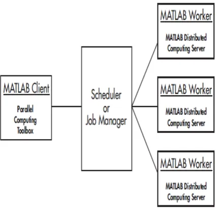
The MATLAB session in which the job and its tasks are defined is called the client session. Often, this is on the machine where you program MATLAB [4, 5]. The client uses Parallel Computing Toolbox software to perform the

definition of jobs and tasks. The MATLAB Distributed

Computing Server™ product performs the execution of your job by evaluating each of its tasks and returning the result to your client session. Parallel Computing Toolbox™ software allows you to run as many as 12 MATLAB workers on your local machine in addition to your MATLAB client session.

C. MATLAB job scheduler (MJS)

(2)

computing configuration is shown in Fig 2.1. The MJS distributes the tasks for evaluation to the server's individual MATLAB sessions called workers. Use of the MJS is optional; the distribution of tasks to workers can also be performed by a third-party scheduler, such as Window HPC Server (including CCS), a Platform LSF scheduler, or a PBS Pro scheduler.

The optional MJS can run on any machine on the network. The MJS runs jobs in the order in which they are submitted, unless any jobs in its queue are promoted, demoted, canceled, or destroyed. Each worker receives a task of the running job from the MJS, executes the task, returns the result to the MJS, and then receives another task. When all tasks for a running job have been assigned to workers, the MJS starts running the next job with the next available worker.

A MATLAB Distributed Computing Server network configuration usually includes many workers that can all execute tasks simultaneously, speeding up execution of large MATLAB jobs. Fig 2.2 shows multiple parallel computing sessions.

A large network might include several MJS sessions as well as several client sessions. Any client session can create, run, and access jobs on any MJS, but a worker session is registered with and dedicated to only one MJS at a time. Fig 2.3 shows multiple MJS processes

As an alternative to using the MJS, you can use a third-party scheduler. This could be a Microsoft Windows HPC Server (including CCS), Platform LSF scheduler, PBS Pro scheduler, TORQUE scheduler, mpiexec, or a generic scheduler. Choosing between a Scheduler and MJS depends on the application.

Figure 2.3 Configuration with Multiple Clients and MJS Processes

Figure 2.4 Life Cycle of a Job

(3)

D. mdce Service

If we are using the MJS, every machine that hosts a worker or MJS session must also run the mdce service [7, 8]. The mdce service recovers worker and MJS sessions when their host machines crash. If a worker or MJS machine crashes, when mdce starts up again (usually configured to start at machine boot time), it automatically restarts the MJS and worker sessions to resume their sessions from before the system crash.

E. Life Cycle of a Job

When we create and run a job, it progresses through a number of stages [9]. Each stage of a job is reflected in the value of the job object’s State property which can be pending, queued, running, or finished. The fig 2.4 below illustrates the stages in the life cycle of a job. In the MJS (or other scheduler), the jobs are shown categorized by their state.

III.PROGRAMDEVELOPMENTUSINGPARALLEL COMPUTINGTOOLBOX

A typical Parallel Computing Toolbox client session includes the following steps:

A. Identify a cluster

Your network may have one or more MJS available (but usually only one scheduler). The function you use to find an MJS or scheduler creates an object in your current MATLAB session to represent the MJS or scheduler that will run your job.

parallel.defaultClusterProfile('local'); c = parcluster();

Here, parallel.defaultClusterProfile indicate we are using the local cluster and parcluster is use to create the object c to represent this cluster.

B. Create a Job

You create a job to hold a collection of tasks. The job exists on the MJS (or scheduler's data location), but a job object in the local MATLAB session represents that job.

Create job j on the cluster by using following syntax.

j = createJob(c)

C. Create Tasks

You create tasks to add to the job. Each task of a job can be represented by a task object in your local MATLAB session. Create as number of tasks we want within the job j. In this example, each task evaluates the sum of the array that is passed as an input argument.

createTask(j, @sum, 1, {[1 1]}); createTask(j, @sum, 1, {[2 2]}); createTask(j, @sum, 1, {[3 3]});

D. Submit a Job to the Job Queue for Execution

When your job has all its tasks defined, you submit it to the queue in the MJS or scheduler. The MJS or scheduler distributes your job's tasks to the worker sessions for evaluation. When all of the workers are completed with the job's tasks, the job moves to the finished state.

submit(j);

E. Retrieve the Job's Results

The resulting data from the evaluation of the job is available as a property value of each task object.

wait(j)

results = fetchOutputs(j)

In this example, it gives result as- results =

[2] [4] [6]

F. Destroy the Job

When the job is complete and all its results are gathered, you can destroy the job to free memory resources.

delete(j)

IV. KEYFEATURESOFTOOLBOXES

A. Parallel for-loops with parfor Keyword

A parfor (parallel for) loop is useful in situations that require many loop iterations of a simple calculation, such as a Monte Carlo simulation. To run parfor we use the Parallel Computing Toolbox. matlabpool sets up a task-parallel execution environment in which parfor loops can be executed interactively from the MATLAB command prompt. The iterations of parfor loops are executed on labs. A lab is an independent instance of MATLAB that runs in a separate operating system process. Commonly, labs execute in headless mode, i.e., they do not have a GUI front end attached to them any of their interaction with the rest of the system happens through messages exchanged through the operating system kernel or a network interconnect. Like threads, labs are executed on processor cores, and the number of labs does not have to match the number of cores. Unlike threads, labs do not share memory with each other. As a result, they can run on separate computers connected via a network.

B. Single Program Multiple Data (spmd)

(4)

execution by each parallel core but each core has its own data to operate on. Unlike parfor loops, spmd blocks (the code between spmd and its corresponding end) require much larger mental leap from sequential loops. The reason is that any code executed inside spmd can behave differently on each core.

C. Distributed Arrays

Distributed arrays are implemented as MATLAB objects where each lab stores a piece of the array. Each piece of this array, in addition to storing the data, also stores information about the type of distribution, the local indices, the global array size, blocking, the number of worker processes, etc. Distributed arrays support two data distributions—one-dimensional distribution and two-distributions—one-dimensional block cyclic distributions. Users have access to various parameters to specify data distributions for their distributed arrays. With MATLAB distributed arrays, users can change distributions as they see fit by redistributing data. Users can even create distributions on the fly by, for example, reading arbitrary portions of data from a file and concatenating individual pieces to construct distributed arrays. Certain operations and math functions can also change data distribution. For example, in the extreme case, the gather operation brings all the data onto a single lab (provided it fits) leaving the rest of the pieces on other labs empty.

D. The Parallel Command Window

A parallel command window (pmode) provides a command line interface to an SPMD programming model with interrupt capability and also displays output from all the computational processes. This interface allows both prototyping and development of SPMD algorithms and interactive use of the distributed array language features. In fact, all the code in the distributed array was developed using the parallel command window. The parallel command window is a relatively simple use of the control layer, where simple evaluation request messages are sent to all labs when a user types a command in the parallel command window. All display output from the labs is streamed back to the client machine using observed return messages (messages are returned from remote processes, received by the I/O infrastructure and are then passed on to designated ‘observers’ for further processing). The parallel command window has display features that allow this output to be viewed in several different ways. Interrupt and other control requests can be sent as messages that are out-of-band and affect all the labs. The only relatively difficult part is ensuring that the state of all the labs remains consistent when a user types a command that might affect one lab differently from others.

V. RUNNINGPARALLELSIMULATIONS

A. Calling sim from within parfor

The MATLAB parfor command allows to run parallel Simulink simulations. Calling sim from within a parfor loop is often advantageous for performing multiple simulation

runs of the same model for different inputs or for different parameter settings. For example, you may save significant simulation time performing parameter sweeps and Monte Carlo analyses by running them in parallel. Running parallel simulations using parfor does not mean decomposing your model into smaller connected pieces and running the individual pieces simultaneously on multiple workers. Normal, Accelerator, and Rapid Accelerator simulation modes are supported by sim in parfor. Specifically, the simulations need to create separately named output files and workspace variables; otherwise, each simulation will overwrite the same workspace variables and files, or possibly have collisions trying to write variables and files simultaneously.

B. Choosing a Simulation Mode

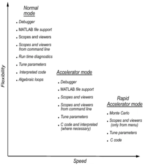
Normal, Accelerator, and Rapid Accelerator simulation models are supported by sim in parfor. In general, choosing between a simulation mode must trade off simulation speed against flexibility. Figure 5.1 shows Speed versus Flexibility measure of different modes.

Normal mode offers the greatest flexibility for making model adjustments and displaying results, but it runs the slowest. Rapid Accelerator mode runs the fastest, but this mode does not support the debugger or profiler, and works only with those models for which C code is available for all of the blocks in the model. In addition, Rapid Accelerator mode does not support 3-D signals. If your model has 3-D signals, use Normal or Accelerator mode instead. Accelerator mode lies between these two in performance and in interaction with your model.

C. sim in parfor with Rapid Accelerator Mode

Running Rapid Accelerator simulations in parfor combines speed with automatic distribution of a prebuilt

(5)

executable to the parfor workers. As a result, this mode eliminates duplication of the update diagram phase. To run parallel simulations in Rapid Accelerator simulation mode using the sim and parfor commands, the following should be done:

• Configure the model to run in Rapid Accelerator

simulation mode

• Ensure that the Rapid Accelerator target is already built and up to date

• Disable the Rapid Accelerator target up-to-date check by setting the sim command option RapidAcceleratorUpToDateCheck to 'off'.

VI. CONCLUSION

With the explicit parallelism provided and use of multicore, multiprocessor and GPU’s Mathwork’s extension to parallel computing has very significant advantage in development of parallel algorithms. The flexibility in using these toolboxes leads to a simple programming. A parallel simulation facility simplifies the testing of the application in some runs. It concludes that with these matlab toolboxes we have a lots of parallel computing features practical.

VII. REFERENCES

[1] Gaurav Sharma, Jos Martin MATLAB: A Language for

Parallel Computing published with open access at

Springerlink.com Int J Parallel Prog (2009)

[2] ww.h.eng.cam.ac.uk/help/tpl/programs/Matlab/parallel.html [3] http://scent.gist.ac.kr/downloads/tutorial/2011/4/Parallel%20C

omputing%20with%20MATLAB(Draft)_MathWorks.pdf [4] http://hpc.kfupm.edu.sa/Documentation/MATLAB%20PARA

LLEL.pdf

[5] http://people.sc.fsu.edu/~jburkardt/presentations/fdi_2009_mat lab.pdf

[6] http://www.american.edu/cas/hpc/upload/AU-Matlab-UserGuide.pdf

[7] http://atc.ugr.es/~javier/investigacion/papers/mpitb_papers.htm l

[8] Moler, C.: Parallel MATLAB: Multiple processors and multiple cores, The MathWorks News and Notes, June 2007