Predicting Missing Items in a Shopping Cart using Positional Mining Algorithm

Volume 2, No. 4, July-August 2011

International Journal of Advanced Research in Computer Science

RESEARCH PAPER

Available Online at www.ijarcs.info

© 2010, IJARCS All Rights Reserved 547

Predicting Missing Items in a Shopping Cart using Positional Mining Algorithm

Kanna Sandhya Laxmi*

Sree Chaitanya College of Engineering Karimnagar, AP,India

sandhya.21k@gmail.com

T.P.Shekhar

Associative Professor, M.Tech CSE Coordinator Sree Chaitanya College of Engineering

Karimnagar, AP, India tpshekhar@gmail.com

K. Sai Krishna

Trinity College of Engineering & Technology Karimnagar, AP, India

Kanna1232@gmail.com

Abstract: Prediction in shopping cart uses partial information about the contents of a shopping cart for the prediction of what else the customer is likely to buy. Existing representation uses Itemset Tree (IT-tree) data structure, all rules whose antecedents contain atleast one item from the incomplete shopping cart generated. This paper uses a new concept of “Positional Lexicographic Tree” (PLT) with which frequ-ent itemsets are generated. Association rules are to be generated from the already generated frequent itemsets by using Positional Mining Algorithm.Then, we combine these rules by using Dempster-Shafer (DS) theory of evid-ence combination. Finally the predicted items are genera-ted to the user.

Keywords: Frequent Itemsets, Association Rule Mining, Positional Lexicographic Tree, Prediction,Positional Mining Algorithm, Dempster-Shafer Theory of Rule Combination.

I. INTRODUCTION

Data Mining refers to extracting or mining information from large amounts of data. Data mining has attracted a great deal of attention in the information industry and in society as a whole in recent years, due to wide availability of huge amounts of data and the imminent need for turning such data into useful information and knowledge.

Data Mining, “the extraction of hidden predictive information from large databases”, is a powerful new technology with great potential to help companies focus on the most important potential to help companies focus on the most important information in their data warehouses. Data mining tools predict future trends and behaviors, allowing businesses to make proactive, knowledge-driven decisions.

The automated, prospective analysis offered by data mining move beyond the analysis of past events provided by retrospective tools typical of decision support systems. Data mining tools can answer business questions that traditionally were too time consuming to resolve. They scour databases for hidden patterns, finding predictive information that experts may miss because it lies outside their expectations.

Most companies collect and refine massive quantities of data. Data mining techniques can be implemented rapidly on existing software and hardware platforms to enhance the value of existing information resources and can be integrated with new products and systems as they are brought on-line. When implemented on high performance client/server or parallel processing computers, data mining tools can be analyze massive databases to deliver answers to many questions.

The information and knowledge gained can be used for application ranging from market analysis, fraud detection, and customer retention, to production control and science exploration. Data mining plays an important role in online

shopping for analyzing the subscribers’ data and understanding their behaviors and making good decisions such that customer acquisition and customer retention are increased which gives high revenue.

A. Association Rule Mining

Association Rule Mining [1] is a popular and well researched method for discovering interesting relations between variables in large databases. Association rules are statements of the form {x1,x2,x3,…..,xn}=>y meaning that if all of x1,x2,x3,…,xn is found in the market basket, and then we have good chance of finding y for us to accept this rule is called confidence of the rule. Normally rules that have a confidence above a certain threshold only will be searched.

The discovery of such associations can help retailers develop marketing strategies by gaining insight into which items are frequently purchased together by customer and which items bring them better profits when placed with in close proximity.

The problem of association rules can be divided into two steps. In the first step, the set of itemsets that exceeds a predefined threshold are determined, these itemsets are called frequent. In the second step, the association rules are determined from this set of frequent itemsets. . For example, a good marketing strategy cannot be run involving items that no one buys. Thus, much data mining starts with the assumption that sets of items with support are only considered. In this paper, we use a new representation for the data stored in the database of the form a lexicographic tree that will be used to enumerate the frequent relations present in large database. Our enhancement is in the way in which this representation makes subset of checking a light process, as well as the applicability of the data to compression and indexing techniques.

the shopping cart of a customer at the checkout counter contains bread, butter, milk, cheese, and pudding. Could someone who met the same customer when the cart contained only bread, butter, and milk, have predicted that the person would add cheese and pudding?

It is important to understand that allowing any item to be treated as a class label presents serious challenges as compared with the case of just a single class label. The number of different items can be very high, perhaps hundreds, or thousand, or even more. To generate association rules for each of them separately would give rise to great many rules with two obvious consequences: first, the memory space occupied by these rules can be many times larger than the original database (because of the task’s combinatorial nature); second, identifying the most relevant rules and combining their sometimes conflicting predictions may easily incur prohibitive computational costs. In this work, both of these problems are solved by developing a technique that answers user’s queries (for shopping cart completion) in a way that is acceptable not only in terms of accuracy, but also in terms of time and space complexity. B. Existing Approach

The existing system uses flagged Itemset trees for rule generation purpose. An itemset tree, T, consists of a root and a (possibly empty) set, {T1; . . . ;Tk}, each element of which is an itemset tree. The root is a pair [s, f(s)], where s is an itemset and f(s) is a frequency. If si denotes the itemset associated with the root of the ith subtree, then s is a subset of si; s not equal to si, must be satisfied for all i. The number of nodes in the IT-tree is upper-bounded by twice the number of transactions in the original database.

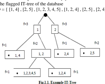
Note that some of the itemsets in IT-tree [4] are identical to at least one of the transactions contained in the original database, whereas others were created during the process of tree building where they came into being as common ancestors of transactions from lower levels. They modified the original tree building algorithm by flagging each node that is identical to at least one transaction. These are indicated by black dots. This is called flagged IT-tree [4]. Here is an example for an IT-tree [4].

The flagged IT-tree of the database

D = { [1, 4] , [2, 5] , [1, 2, 3, 4, 5] , [1, 2, 4] , [2, 5] , [2, 4] is

Here some items in this tree are flagged to represent them as weak entity so that they are not carried for the next stage of processing.

The disadvantages of Existing approach are:

Time taken to generate association rule in the case of IT-tree is more when compared with the association rules generated with Positional Lexicographic Tree (PLT).

This method requires more memory for processing IT-Tree and generating association rules.

C. Dempster’s Rule of Combination

Dempster’s rule of combination (DRC) [6] is used to combine the discovered. When searching for a way to predict the presence of an item in partially observed shopping carts, association rules are used. However, many rules with equal antecedents differ in their consequents and some of these consequents contain the desired item to be predicted, others do not. The question is how to combine (and how to quantify) the potentially conflicting evidences. DRC [6] is used for this purpose. Finally the predicted items are suggested to the user.

II. PROPOSEDAPPROACH

Figure1. Shows the shopping cart prediction architecture in which the positional lexicographic tree is generated. The frequent itemsets are generated by using Top down Approach. At this stage we need the Support value. Then association rules are to generated from the already generated frequent itemsets. It takes minimum confidence from the user and discovers all rules with a fixed antecedent and with different consequent. The association rules generated form the basis for prediction.

We assign BBA [2] value to each association rule generated. This gives more weight to rules with higher support masses are assigned based on both their confidence and support values.

The incoming itemset i.e the content of incoming shopping cart will also be represented by a Positional vector and positional mining algorithm with each transaction vector ation to generate the association rules. Finally the rules are combined to get the predictions.

Figure 2. Shopping cart prediction architecture

Dempster’s rule of combination (DRC) [6] is used to combine the evidences. When searching for a way to predict the presence or absence of an item in a partially observed shopping cart s, we wanted to use association rules.

Data _{Build Positional Lexicographic Tree}

Frequent Itemset generation by using Top down approach

Association Rule by using Positional Mining Algorithm

BBA and Rule Selection

Decision Making (Dempster’s combination)

Prediction Incoming

Instance

© 2010, IJARCS All Rights Reserved 549 However, many rules with equal antecedents differ in

their consequents—some of these consequents contain the desired item to be predicted, others do not. The question is how to combine (and how to quantify) the potentially conflicting evidences. DRC [6] is used for this purpose. Finally the predicted items are suggested to the user.

III. POSITIONALSTRUCTURALMODEL

In this paper, a new annotation for the lexicographic tree is introduced. This new presentation allows data to be stored in a compressed form and provides an easy mechanism to move between the elements of the tree and an easy way for subset checking during the mining process. Let I = {i1, i2, …in} be a set of items. A lexicographic order is assumed to exist among the items of I; a lexicographic prefix tree is a tree representation where the root node is labeled with null and all other nodes represent elements in the set I listed in lexicographic order from left to right. Each node islinked to the nodes that represent the items that occur after it in the lexicographic order. Figure2. Illustrates the lexicographic tree of the set {A, B, C, D}.

Figure 3. The lexicographic tree of items {A, B, C, D}

A. Basic Definitions

Definition 3.1.1:

Rank (i) is a function that maps each element ( i ∈ I) to a unique integer in such a way that the lexicographic order is maintained.

Definition 3.1.2:

pos(n) is a function that maps each node in the lexicographic tree to an integer that represents its position among its siblings to the parent node starting from left to right.

For example, in Figure2. node C is a child of node A at level 2 and pos(C) = 2 ( i.e. C is in the position of two lexicographically as a child of A).

Definition 3.1.3:

Let Xk be a node at level k. V(Xk) = [pos(x1),

pos(x2),……,pos(xk)] is then a position vector that encodes

the position values of the nodes that formulate the path from the root to node Xk.

Lemma 3.1.1

Let X ={x1, x2,…..,xk} be an itemset and let V(X) =

[pos(x1), pos(x2), ……,pos(xk)] be the corresponding position vector of X . For each xi in X, itthen holds

Rank(xi) = Lemma 3.1.2.

For each subset X ∈ P(I), P(I) is the power set of the set

I, V(X) uniquely determines itemset X in the positional

lexicographic tree. Property 3.1.1

Let Tik be a sub-tree rooted with item I at level k in the Lexicographic Tree Let j be the parent of node i. Tik then has n-repeated structures (subtrees) at level (k+1) within the same sub-tree rooted with node j, where n is the number of siblings that proceed item i in the lexicographic tree according to parent j. eferring once again to Figure 3. The sub-tree rooted with node B in level 1 has the same structure under its left sibling (node A) at level 2.

Lemma3.1.3

Let V(X) = [pos(x1), pos(x2),……,pos(xk)] be a position vector of size k. The position vector representation of any “k-1” level subset of itemset X then has one of the following Figure 3.2. The PLT structure forms:

a) [pos(x1), pos(x2),……,pos(xk-1)] or

b)[pos(x1),pos(x2),…,pos(xi)+pos(xi+1)…,pos(xk] for a given 1<= i <k. That is, the position vector of a potential subset of X at level k-1 is achieved by replacing two consecutive positions in V(X) with their sum.

Figure 4. The PLT structure

Now the complete process of constructing the PLT can be represented. We begin by providing an illustrative example followed by a formula description of the algorithm.

Table 1 shows a database of 8 transactions. In the first step, the database is scanned to determine the set of frequent 1-itemset. Since the only frequent items can participate in formulating the frequent itemsets, this step aims to eliminate those items that less support than the user’s predefined minimum support. Assume that the absolute support count is 2. The set of frequent 1 items are then{(C,4),(D,5),(E,7),(F,8),(G,5)}. The numbers beside the item refer to its frequency. The next step is to associate a unique number with each item using the Rank function. As a result we have: Rank(C) =1, Rank(D) = 2, Rank(E) = 3, Rank(F) = 4, Rank(G)=5.

In the second step, another scan of the database is conducted; for each transaction, the set of infrequent items is filtered out and a Positional vector is created and inserted in a table according to its length (we assume that a table-like data structure is used to represent the positional tree; a physical tree may also be assumed).

1

1 3

3

2

2 4

1 2

1

1

1

2

1

1 A

B D

C

C

B D

C D

C

D

D

D

D

© 2010, IJARCS All Rights Reserved 550 Table I. Transaction DataBase

TID ItemSet

1 ABEF

2 ABEFG

3 CDEF

4 DEFG

5 ABFG

6 CDEFG

7 CDEFG

8 CDEF

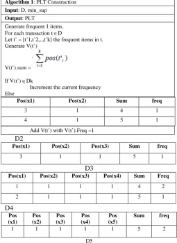
If this vector in a Transaction Data Base previously existed we merely increment its frequency. Otherwise, we simply add it with a support count equal to 1. In other words, we partition the database to a set of partitions such that each partition stores the vectors of the same length. In addition, we store the summation of the position values presented in the vector with each vector. This value will be used during the mining procedure using the conditional approach. A figure 4(a), 4(b) provides two different perspectives for the data using the tree structure and the matrix structure. Algorithm 1 gives the formula specification for the positional tree construction process.

Algorithm 1: PLT Construction Input: D, min_sup

Output: PLT

Generate frequent 1 items. For each transaction t ∈D

Let t’ = [t’1,t’2,..,t’k] the frequent items in t. Generate V(t’)

V(t’).sum =

If V(t’) ∈Dk

Increment the current frequency Else

Pos(x1) Pos(x2) Sum freq

3 1 4 1

4 1 5 1

Add V(t’) with V(t’).Freq =1 D2

Pos(x1) Pos(x2) Pos(x3) Sum freq

3 1 1 5 1

D3

Pos(x1) Pos(x2) Pos(x3) Pos(x4) Sum Freq

1 1 1 1 4 2

2 1 1 1 5 1

D4 Pos (x1)

Pos (x2)

Pos (x3)

Pos (x4)

Pos (x5)

Sum freq

1 1 1 1 1 5 2

D5

Figure 4 (a) The Matrices Structure

Figure 4(b): The Tree Structure

B. 3.2. The PLT Mining Process

It is clear that the support count of any itemset is equal to the number of times it occurs as a single transaction plus the number of transactions in which occurs as a subset. The next two subsections discuss how the positional lexicographic tree can be used during the mining process using the approach Top down.

a. The Top Down Approach

In this methodology, we start with the database partition that represents the itemset of maximum length. For example

k. Then for each entry presented in Dk of the form

[p1,p2,….,pk] with ps as positional values, we generate the vectors of the first two subsets at level k-1 as follows: i. The first subset is constructed based on lemma 3.1.3.a

by removing the last positional value (pk)

ii. The second subset is constructed by replacing (pk and pk-1) by their sum, lemma 3.1.3.b.

For reasons of efficiency and correctness, we may include the first step above in the positional tree construction process since we need this step only for the already existed vectors not for those that are generated using part B above. This is done by adding the vector at different levels in the database by considering one position at a time. For instance, vector [1,1,1,1] should be added as [1,1,1], [1,1] at D3 and D2 partitions. In this case, the top down approach is started by considering part B above and constructing the vector [p1,p2,….,pk-1+pk] and adding it to the Dk-1 partition. The same thing is done for all the vectors in Dk and the vectors in the other partitions by considering the last two positions. After this, part B from above is repeated, but this time the process occurs by shifting one position to the left (i.e. the pair (pk-2, pk-1) for level k). The new vector is [p1,p2,..,pk-1+pk-2,pk], and the same is the case for all other partitions one shift to the left from the pervious location considered; any vector that does not have enough space for shifting has already gone through the mining process. The entire process will continue until there is no longer enough space to shift in any vector. The same condition should be applied to the vectors that were generated in previous iteration if they can satisfy the shifting (i.e. consecutive positional can be added). In this way, all of the subsets are generated and frequency support is inherited by the subsets without duplications.

Algorithm 2:Top Down Approach Input: PLT Structure

Output: All Subsets with their frequencies k = Maximum Vector Length. For j = k down to 2

L=j

1

1

3

2 4

1

1 1

1

1

1

1

1

© 2010, IJARCS All Rights Reserved 551 For i = k down to 2

For each V ∈Di If pL exist in V p’ = pL + pL-1

V’ = V | p’ replaced by pL,pL-1 If V’ ∈Di-1 then

V’.Freq += V.Freq Else

Add V’ with V’.Freq = V.Freq L=L-1

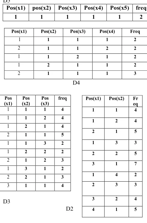
At the end of the above procedure, the database contains all the frequencies of all the subsets that may be presented in the database, and the frequent items are those that have frequency grater than the predefined minimum support. Figure 4 shows the database after the above procedure has been applied to the database in Table 1. We assumed that part A was constructed during the constructions process. Algorithm 2 presents the formula specification for part B. D5

Pos(x1) pos(x2) Pos(x3) Pos(x4) Pos(x5) freq

1 1 1 1 1 2

Pos(x1) Pos(x2) Pos(x3) Pos(x4) Freq

1 1 1 1 2

2 1 1 2 2

1 1 2 1 2

1 2 1 1 2

2 1 1 1 3

D4

D3

D2

Figure 5. The database after top-down approach

C. Association Rule Generation

This module is used to generate association rules from the already generated frequent itemsets.

This algorithm is capable of finding all association rules with a fixed antecedent and with different consequents from the frequent itemsets subject to a user specified minimum confidence very quickly. It takes minimum confidence from the user and discovers all rules with a fixed antecedent and with different consequent. This module also takes the frequent item set and the incoming shopping cart instance to generate the association rule with the corresponding support and confidence value.

Let R denote the root of ‘PLT’ and let ci be R’s children. Let PLTi denote the subtree whose root is ci . In a positional Mining Algorithm, PLT tree generated after applying Top down Approach, Incoming itemset related positional vector sL, where ‘L’ represent size of sL. ‘G’ consisting the rules obtained. Initially it is empty. Comparing the each children of the root with first value in the sL. if it is equal with any one of the children then again traverse towards its children which is equal to second positional value in the sL, else, no rule is generated . The process is continued till the value of j is ‘L’ . finally checking whether ci is having children or not. If yes, no rule is generated; otherwise the rules are generated by using Update ( ) function.

Algorithm3: Positional Mining :Algorithm that process Positional Lexicographical Tree (PLT) and returns Assocition Rules with fixed antecedent that predicts unseen items in a user-specified itemset sl Input: PLT, sL

j=1

G=Positional_Mining( PLT,sj,{} ) If j<=Land PLT non-empty If ci=si for some i do If j<L

G Positional_Mining(PLTi,sj+1,G) Else

If ci does not have children No rule is generated Else

Sum=0

G Update(PLTi,G,sum,L) Endif

Endif Endif Endif End

Update((PLTi,G,sum,j): For each ci do

Generate (sk)k=1 to j ci+sum ,

support=freq(Rule) / Total no. of transaction in the DataBase

confidence=freq(Rule)/freq(sL)

If ci have children

GUpdate(PLTi,G,sum+ci, j) Endif

Endfor end

Incoming vector = (c,d) //positional vector of (c,d)= (1,1) Confidence=80%

Table 2: Rule Generation Output

Positional Vector

Rule Support confidence

(1,1 ; 1) (c,d)=>e 0.5 1

(1,1 ; 2) (c,d)=>f 0.5 1

D. 3.5 BBA and Decision Making

a. Partitioned-Support

In many applications, the training data set is skewed. Thus, in a supermarket scenario, the percentage of shopping carts containing, say canned fish, can be 5 percent, the remaining 95 percent shopping carts not containing this item. Pos

(x1) Pos (x2)

Pos (x3)

freq

1 1 1 4

1 1 2 4

1 2 1 4

2 1 1 5

1 1 3 2

1 2 2 2

2 1 2 3

1 3 1 2

2 2 1 3

3 1 1 4

Pos(x1) Pos(x2) Fr

eq

1 1 4

1 2 4

2 1 5

1 3 3

2 2 5

3 1 7

1 4 2

2 3 3

3 2 4

Hence, the rules that suggest the presence of canned fish will have very low support while rules suggesting the absence of canned fish will have a higher support.

Unless compensated for, a predictor built from a skewed training set typically tends to favor the “majority” classes at the expense of “minority” classes. In many scenarios, such a situation must be avoided. To account for this data set skewness, we propose to adopt a modified support value termed partitioned-support. The partitioned-support p_supp of the rule, r (a) -> r(c), is the percentage of transactions that contain r (a) among those transactions that contain r(c), i.e.,

p_supp = support(r (a) U r(c)) / support(r(c))

b. BBA:

In association mining techniques, a user-set minimum support decides about which rules have “high support.” Once the rules are selected, they are all treated the same, irrespective of how high or how low their support. Decisions are then made solely based on the confidence value of the rule. However, a more intuitive approach would give more weight to rules with higher support. Therefore, we use a novel method to assign to the rules masses based on both their confidence and support values. This weight value is called Basic Belief Assignment (BBA) [2].

We assign BBA value to each association rule generated.

β = ((1+α2 ) x conf x p_supp ) / (α2 x conf + p_supp); α € [0,1];

Dempster’s rule of combination (DRC) [6] is used to combine the evidences. When searching for a way to predict the presence or absence of an item in a partially observed shopping carts, we wanted to use association rules. However, many rules with equal antecedents differ in their consequents—some of these consequents contain the desired item to be predicted, others do not. The question is how to combine (and how to quantify) the potentially conflicting evidences. DRC [6] is used for this purpose. Some illustrations used from DRC [6] are explained in following paragraph.

We remove the overlapping rules while keeping the highest confidence rule. If two overlapping rules have the same confidence, the rule with the lower support is dropped. Finally the best rule is selected by comparing the mass values. The predicted item is then suggested to the user.

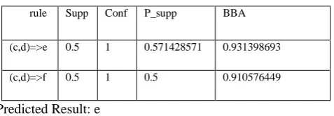
The input given to this stage is the set of rules generated along with their support and confidence values as shown in the below table 2.

Table 3: BBA & Decision Making Output

rule Supp Conf P_supp BBA

(c,d)=>e 0.5 1 0.571428571 0.931398693

(c,d)=>f 0.5 1 0.5 0.910576449

Predicted Result: e

The table 3 shows the output of this stage i.e., the calculated BBA[6] values. The prediction made is also shown below the table.

IV. CONCLUSION

The Top-Down Approach algorithm is used to generate frequent itemsets and positional mining algorithms is used to

generate Association Rules. Association rules formed the basis of prediction. The algorithm is applied in a demo shoppingcart application. When user adds each item to the cart the algorithm is executed and the prediction is displayed. The advantages of the proposed work are:

A. It is also effiecient in the case of large databases.

B. PLT provides partition criteria that makes it easy to position the mining process into several separate tasks; each can be accomplished separately.

C. Processing speed is more when compared to the rules generated using itemset tree and DS theory.

D. It is better than Apriori algorithm which required several datastructures during mining process, where as, PLT is considered to be self-continued structure. (i.e., no data structure is required during mining process.

V. FUTUREENHANCEMENT

The Top-Down Approach algorithm is applicable where a very low minimum support is provided. Our future research will explore the conditional approach to generate frequent itemsets which is used in case of high support count is required.

VI. REFERENCES

[1]. Kasun Wickramaratna, Miroslav Kubat and Kamal Premaratne, “Predicting Missing Items in Shopping Carts”, IEEE Trans. Knowledge and Data Eng., vol. 21, no. 7, july 2009.

[2]. M.Anandhavalli, Sandip Jain, Abhirup Chakraborti, Nayanjyoti Roy and M.K.Ghose “Mining Association Rules Using Fast Algorithm”, Advance Computing Conference (IACC), 2010 IEEE 2nd International. [3]. H.H. Aly, A.A. Amr, and Y. Taha, “Fast Mining of

Association Rules in Large-Scale Problems,” Proc. IEEE Symp. Computers and Comm. (ISCC ‟01), pp. 107-113, 2001.

[4]. R. Agrawal and R. Srikant, “Fast Algorithms for Mining Association Rules,” Proc. Int‟l Conf.Very Large Databases (VLDB ‟94), pp.487-499, 1994.

[5]. K.K.R.G.K. Hewawasam, K. Premaratne, and M.-L. Shyu, “Rule Mining and Classification in a Situation Assessment Application: A Belief Theoretic Approach for Handling Data Imperfections,” IEEE Trans. Systems, Man, Cybernetics, B, vol. 37, no. 6 pp. 1446-1459, Dec. 2007.

[6]. Apriori Algorithm Reference URL:

http://www2.cs.uregina.ca/~dbd/cs831/notes/itemsets/ite mset_prog1.html

[7]. R. Agrawal, T. Imilienski, A. Swami. Mining association rules between sets of items in large databases. In proceedings of the ACM SIGMOD international conference on Management of data, PP: 207-216, 1993.Panther, J. G., Digital Communications, 3rd ed., Addison-Wesley, San Francisco, CA (1999). [8]. P. Bollmann-Sdorra, A. Hafez, and V.V. Raghavan, “A

Theoretical Framework for Association Mining Based on the Boolean Retrieval Model,” Data Warehousing and Knowledge Discovery: Proc. Third Int’l Conf. (DaWaK ’01), pp. 21-30, Sept. 2001.

© 2010, IJARCS All Rights Reserved 553 Querying,” IEEE Trans. Knowledge and Data Eng., vol.

15, no. 6, pp. 1522-1534, Nov./Dec. 2003.

[10].K.K.R.G.K. Hewawasam, K. Premaratne, and M.-L. Shyu, “Rule Mining and Classification in a Situation Assessment Application: A Belief Theoretic Approach for Handling Data Imperfections,” IEEE Trans. Systems, Man, Cybernetics, B, vol. 37, no. 6 pp. 1446-1459, Dec. 2007.

[11].B. Liu, W. Hsu, and Y.M. Ma, “Integrating Classification and Association Rule Mining,” Proc.

ACM SIGKDD Int’l Conf. Know. Disc. Data. Mining (KDD ’98), pp. 80-86, Aug. 1998.

[12].R. Agarwal, C.Aggarwal, and V. Prasad. A tree projection algorithm for generation of frequent itemsets. Journal Parallel and Distributed Computing, 2000. [13].M. EL-Hajj, O.R Zaiane. Non Recursive Generation of