Classification of Epileptic EEG Using Wavelet Transform & Artificial Neural Network

(1)

Volume 4, No. 9, July-August 2013

International Journal of Advanced Research in Computer Science

RESEARCH PAPER

Available Online at www.ijarcs.info

ISSN No. 0976-5697

Classification of Epileptic EEG Using Wavelet Transform & Artificial Neural Network

Ashish Raj1, Manoj Kumar Bandil2, D B V Singh3, Dr. A.K Wadhwani4

[email protected],[email protected],[email protected],[email protected]

Abstract— Epilepsy is a neurological disorder with prevalence of about 1-2% of the world’s population. The hallmark of epilepsy is recurrent seizures termed "epileptic seizures". Human Brain is the most complex organ among all the systems in the human body, also the most remarkable one. It exhibits rich spatiotemporal dynamics. Electroencephalography (EEG) signal is the recording of spontaneous electrical activity of the brain over a small period of time . The term EEG refers that the brain activity emits the signal from head and being drawn. It is produced by bombardment of neurons within the brain. EEG signal provides valuable information of the brain function and neurobiological disorders as it provides a visual display of the recorded waveform and allows computer aided signal processing techniques to characterize them. This gives a prime motivation to apply the advanced digital signal processing techniques for analysis of EEG signals. The main objective of our research is to analyze the acquired EEG signals using signal processing tools such as wavelet transform and classify them into different classes. The features from the EEG are extracted using statistical analysis of parameters obtained by wavelet transform. After feature extraction secondary goal is to improve the accuracy of classification. Total 300 EEG data subjects were analyzed. These data were grouped in three classes’ i.e, Normal patient class, Epileptic patient class and epileptic patient during non-seizure zone respectively. In order to achieve this we have applied a backpropgation based neural network classifier. After feature extraction secondary goal is to improve the accuracy of classification. 100 subjects from each set were analysed for feature extraction and classification and data were divided in training, testing and validation of proposed algorithm.

Index Terms— EEG, Epilepsy, Wavelet transform; Feature Extraction, Neural network, Backpropogation Neural Network.

I. INTRODUCTION

Monitoring brain activity through the electroencephalogram (EEG) has become an important tool in the diagnosis of epilepsy. The EEG recordings of patients suffering from epilepsy show two categories of abnormal activity: inter-ictal, abnormal signals recorded between epileptic seizures; and ictal, the activity recorded during an epileptic seizure. The EEG signature of an inter-ictal activity is occasional transient waveforms, as either isolated spikes, spike trains, sharp waves or spike-wave complexes. EEG signature of an epileptic seizure (ictal period) is composed of a continuous discharge of polymorphic waveforms of variable amplitude and frequency, spike and sharp wave complexes, rhythmic hyper synchrony, or electro cerebral inactivity observed over a duration longer than the average duration of these abnormalities during inter-ictal periods. During inter-ictal periods, or between epileptic seizures, EEG recordings of patients affected by epilepsy will exhibit abnormalities like isolated spike, sharp waves and spike- wave complexes (usually all termed as inter-ictal spikes or spikes). In ictal periods, or during epileptic seizures, the EEG recording is composed of a continuous discharge of one of these abnormalities, but extended over a longer duration and typically accompanied by a clinical correlate.[1]

Generally, the detection of epilepsy can be achieved by visual scanning of EEG recordings for inter-ictal and ictal activities by an experienced neurophysiologist. However, visual review of the vast amount of EEG data has serious drawbacks. Visual inspection is very time consuming and inefficient, especially in the case of long-term recordings. In addition, disagreement among the neurophysiologists on the same recording is possible due to the subjective nature of

the analysis and due to the variety of inter-ictal spikes morphology.

Moreover, the EEG patterns that characterize an epileptic seizure are similar to waves that are part of the background noise and to artifacts (especially in extra cranial recordings) such as eye blinks and other eye movements, muscle activity, electrocardiogram, electrode "pop" and electrical interference. For these reasons, methods for the automated detection of inter- ictal spikes and epileptic seizures can serve as valuable clinical tools for the scrutiny of EEG data in a more objective and computationally efficient manner.[1]

(2)

dt nb t a t f a t

x

w m m

n m n

m (), () ( 0() 0)

2 / 0 ,

[image:2.595.39.254.52.232.2]

, =

ψ

=

∫

ψ

−

Figure 1.1. Computation process of DWT

The standard equation of Discrete Wavelet Transform is given as-

(1.1) Where sub wavelets is given by-

(1.2) The DWT decomposition can be described as

= ∗ , ( )

where a(k)(l) and d(k)(l) are the approximation coefficie nts and the detail coefficients at resolution k, respectively.

The wavelet transform gives us multi-resolution description of a signal. It addresses the problems of non-stationary signals and hence is particularly suited for feature extraction of EEG signals [2]. At high frequencies it provides a good time resolution and for low frequencies it provides better frequency resolution, this is because the transform is computed using a mother wavelet and different basis functions which are generated from the mother wavelet through scaling and translation operations. Hence it has a varying window size which is broad at low frequencies and narrow at high frequencies, thus providing optimal resolution at all frequencies.

b. Data base- The raw EEG signal is obtained from university of Bonn which consists of total 5 sets (classes) of data (SET A, SET B, SET C, SET D, and SET E) corresponding to ﬁve diﬀerent pathological and normal cases. Three data sets are selected from 5 data sets in this work. These three types of data represent three classes of EEG signals (SET A contains recordings from healthy volunteers with open eyes, SET D contains recording of epilepsy patients in the epileptogenic zone during the seizure free interval, and SET E contains the recordings of epilepsy patients during epileptic seizures)

All recordings were measured using Standard Electrode placement scheme also called as International 10-20 system. Each data set contains the 100 single channel recordings. The length of each single channel recording was of 26.3 sec.The 128 channel ampli ﬁer had been used

for each channel [3]. The data were sampled at a rate of 173.61 samples per second using the 12 bit ADC. So the total samples present in single channel recording are nearly equal to 4097 samples (173.61×23.6). The band pass ﬁlter was ﬁxed at 0.53-40 Hz (12dB/octave) [4].

II. METHODOLOGIES

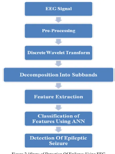
DWT successfully analyses the multi-resolution signal at different frequency bands, by decomposing the signal into approximation and detail information. The method for frequency band separation for epilepsy detection is implemented in MATLAB 2013a. The flowchart of the proposed methodology for detection of epileptic data from normal data is shown in figure Epilepsy Detection using EEG requires feature extraction from the acquired signal in specific frequency range of delta, theta, alpha, beta, and gamma. Though some researchers have mentioned the use of DWT decomposition to obtain these bands, the method given is inadequate to achieve these. First this study explicitly describes the method of up-sampling and recombining of several decomposed sub bands to achieve the required frequencies. Data is first pre-processed by removing dc component from the signal thereby achieving different levels of decomposition for Daubechies order-2 wavelet with a sampling frequency of 173.6 Hz on each signal of 4096 samples.

The overall process can be explained using following flowchart-

Figure 2.1Steps of Detection Of Epilepsy Using EEG

a. Feature Extraction – From the data available at [9 ] a rectangular window of length 256 discrete data was selected to form a single EEG segment. For analysis of signals using Wavelet transform selection of the appropriate wavelet and number of decomposition level is of utmost importance. The wavelet coefficients were computed using daubechies wavelet of order 2 because its smoothing features are more suitable to detect

Z n m nb

t a a

t m m

n

m ( )= ( 0( )− 0) , ∈

2 / 0

, ψ

[image:2.595.334.537.404.676.2]

(3)

changes in EEG signal. In the present study, the EEG signals were decomposed into details D1-D5 and one approximation A5. After calculating coefficients we can calculate various features using statistical analysis of coefficients. [4]

[image:3.595.319.552.53.636.2]

The feature extraction is shown in fig 2.2-

Figure 2.2 Feature Extraction using DWT

A rectangular window of length 256 discrete samples is selected from each channel to form a single EEG segment. The total numbers of time series present in each class are 100 and each single channel time series contained 16 EEG signal segments. Therefore total 1600 EEG segments are produced from each class. Hence, total 4800 EEG segments are obtained from three classes. The 4800 EEG segments are divided into training and testing data sets. The 2400 EEG signal segments (800 vectors from each class) are used for testing and 2400 EEG signal segments (800 segments from each class) are used for training.[5]

b.Normalization and Segment Detection:

a) Normalization- Each recorded signals of all the 3 classes are normalized to -1 and +1 value. This is done by dividing all the samples with the maximum absolute value. The matlab command for normalization of signals is given as-

>>signal_normalized=signal/max (abs (signal)); The normalized plot of Raw EEG signals are shown as below.

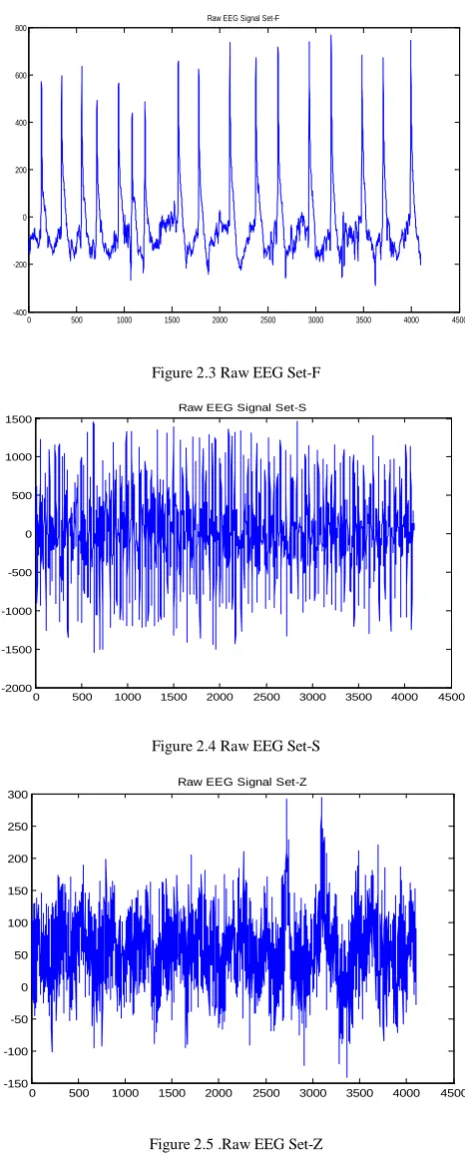
b) Segment Detection- A rectangular window of length 256 discrete samples is selected from each channel to form a single EEG segment. The total numbers of time series present in each class are 100 and each single channel time series contained 16 EEG signal segments. Therefore total 1600 EEG segments are produced from each class. Hence, total 4800 EEG segments are obtained from three classes. The 4800 EEG segments are divided into training and testing data sets. The 2400 EEG signal segments (800 vectors from each class) are used for testing and 2400 EEG signal segment (800 segments from each class) are used for training.[8] The plots for the segment of three dta sets is given below-

0 500 1000 1500 2000 2500 3000 3500 4000 4500 -400

-200 0 200 400 600 800

Raw EEG Signal Set-F

Figure 2.3 Raw EEG Set-F

0 500 1000 1500 2000 2500 3000 3500 4000 4500

-2000 -1500 -1000 -500 0 500 1000 1500

Raw EEG Signal Set-S

Figure 2.4 Raw EEG Set-S

0 500 1000 1500 2000 2500 3000 3500 4000 4500

-150 -100 -50 0 50 100 150 200 250 300

Raw EEG Signal Set-Z

Figure 2.5 .Raw EEG Set-Z

Figure 2.3,2.4 and 2.5 shows the plot of raw EEG signals from the given set of data. These signals were analyzed using matlab to decompose it using DWT with db2 as mother wavelet and the level of decomposition as 5. The MATLAB commands used for the feature extraction are as follows-:

Table.1.Matlab Commands

Signal Processing Tool MATLAB Command

[image:3.595.43.271.125.326.2]

(4)

Table.2 List of Wavelet based Features for One Sample of Each Set

S.No. Name of Feature Set-F Set-S Set-Z

1 Maximum value of Detail Coefficient D1

359.174 782.209 764.113

12.986 45.186 27.736

33.821 174.180 107.435

91.007 368.487 191.755

114.330 707.499 194.409

6 Maximum value of Detail Coefficient A5

168.054 911.882 277.955

7 Mean of Detail coefficients M11

100.711 186.958 160.348

2.3148 8.001 6.582

6.065 32.561 22.431

15.318 104.711 46.333

28.601 272.962 63.768

12 Mean of Approx. coefficients M16

55.097 186.958 160.348

13 Variance of Detail coefficients V11

16086.408 69850.410 45818.690

8.464 122.109 68.255

59.575 1994.245 786.792

378.563 18354.180 3360.195

1420.164 108091.930 6561.674

18 Variance of Approx.l coefficients

V16

5019.397 141019.303 12344.644

19 Standard Deviation of Detail coefficients

S11

126.832 264.292 214.053

S12

2.909 11.052 8.261

S13

7.718 44.656 28.049

S14

19.456 135.477 57.967

S15

37.685 328.773 81.004

24 Standard Deviation of Apporx. coefficients

S15

70.847 375.525 111.106

25 Inter-Quartile Range 42 181.250 67.250

The features calculated from the given set of data was collected together to form a feature vector of 25 features for 300 samples of data.

After feature extraction we classified the data with neural network classifier to develop an efficient classification

(5)

III. CLASSIFICATION USING NEURAL NETWORK

In our research work we have implemented classification of Epileptic EEG with help of Scaled Conjugate-Back Propagation Neural Network with hidden layer equal to 10 and initial weights assumed to be zero. For classification of features using neural network we need two important pre-defined parameters which are as follows-[9]

a) Input Vector b) Target Vector

a. Input Vector- In our research the feature vector was implemented as input vector. This input vector consists of a matrix of size 25X300 such that rows indicate the features and column indicates number of samples. The overview of input vector is discussed as follows- (a). Number of rows = 25 (Representing number of

features of the samples as explained in table ) (b). Number of columns=300 (Representing number of

respective samples taken for training, testing and validation of Neural Network Classifier).

i.Set-F-100 Samples (Epileptic Patients during Seizure Free Interval)

ii.Set-S-100 Samples (Epileptic Patients during Seizure)

iii.Set-Z-100 Samples (Normal Patients without Seizure)

b. Target Vector- In our research the results was implemented as target vector. This target vector consists of a matrix of size 3X300 such that rows indicate the target class and column indicates number of samples to be tested. The overview of target vector is discussed as follows-

(a). Number of rows = 3 (Representing number of features of the samples as explained in table ) i.Class 1 – Epileptic Patient without Seizures- (1 0 0) ii.Class 2 – Epileptic Patient during Seizures- (0 1 0) iii.Class 3 – Normal Patients without Seizures - (0 0 1)

(b). Number of columns=300 (Representing number of respective samples taken for training, testing and validation of Neural Network Classifier).

[image:5.595.312.558.337.762.2]

The overall classification was done using input vector and target vector with scaled conjugate gradient based back propagation neural network.

Figure 3.1.Model of Neural Network

In our classification process there are 25 input layers with 10 hidden layer and 3 output neurons for wavelet based features.

a) Input Neurons = Number of features b) Output Neuron = Number of Target Classes.

IV. RESULTS

Using MATLAB R2013a the overall classification was done using SCGA based Back propagation Neural Network Classifier. The results are shown as follows-

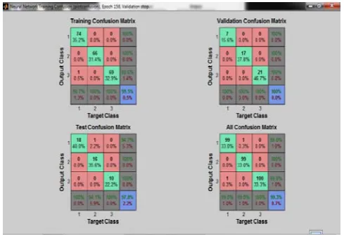
The overall Confusion Matrix for the given neural network is shown below-

Table-3

Type of Dataset Accuracy

Set-F(Epileptic Patient without Seizures) 99% Set-S(Epileptic Patient with Seizures) 100% SetZ (Healthy Patient without Seizures) 99%

Overall Accuracy of the Network 99.3%

The overall samples are divided into three categories- i.Training Data-70 % of total dataset.

ii.Testing Data- 15 % of total dataset. iii.Validation Data- 15 % of total dataset.

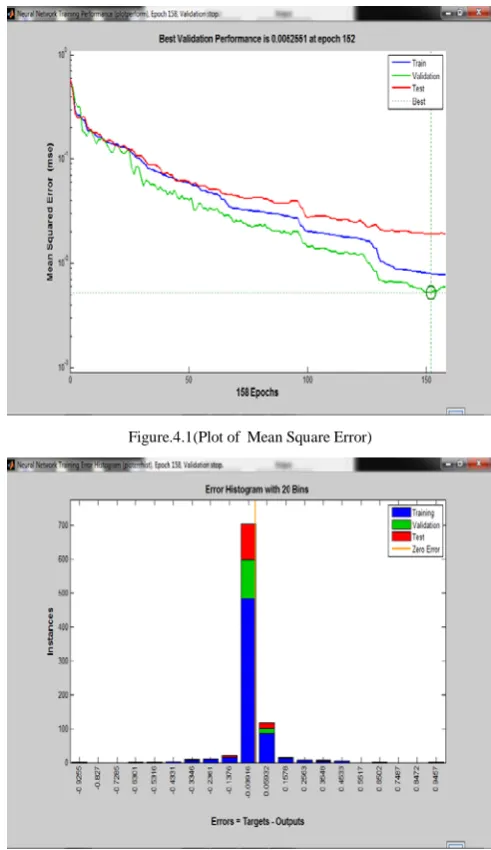
The Results is illustrated using graphs which are listed below-:

Figure.4.1(Plot of Mean Square Error)

[image:5.595.42.274.576.743.2]

(6)

[image:6.595.34.279.52.220.2]

Figure 4.3. (Confusion Matrix for Neural Network)

V. COCNLUSIONS

In our research we have designed a soft computing based expert system for classification of epileptic and non epileptic EEG signals of 300 samples of data. The overall conclusion can be summarized in following points-:

a. An Automated Epileptic Classification system is developed using Statistical features extraction and Soft Computing based classification tool.

b. Total 300 samples of individual patients were analyzed as 100 samples from each Epileptic, Pre-epileptic and Normal patients.

c. Total 25 features for wavelet features were selected to develop features input vector for classifier.

d. Classification process is carried out using SCGA- Back Propagation Neural Network Classifier. e. Overall efficiency of 99 percent is achieved in the

classification process .

VI. REFERENCES

[1]. Automated Epileptic Seizure Detection Methods: A Review Study, Alexandros T. Tzallas, Markos G. Tsipouras, Dimitrios G. Tsalikakis, Evaggelos C. Karvounis, Loukas Astrakas, Spiros Konitsiotis and Margaret Tzaphlidou Department of Medical Physics, Medical School, University of Ioannina, Ioannina, Greece,2011

[2]. Elif Derya Übeyli,(2009), ―Statistics over Features: EEG signals analysis‖, Computers in Biology and Medicine, Vol. 39, Issue 8, 733-741

[3]. Daubechies, “The wavelet transform, time-frequency local ization and signal analysis,”IEEE Trans. on Information Theory, vol. 36, no.5, pp. 961-1005, 1990.

[4]. Adaptive neuro-fuzzy inference system for classiﬁcation of EEG signals using wavelet coefﬁcientsInan Guler ,Elif Derya Ubeyli Journal of Neuroscience Methods Elsevir (2005)

[5]. E. D. U beyli, “Wavelet/mixture of experts network structure for EEG signals classiﬁ - cation,” Expert Systems with Applications, vol. 34, pp. 1954-1962, 2008.

[6]. E. D. U beyli, “Least squares support vector machine employing model-based methods coeﬃcients for analysis of EEG signals,” Expert Systems with Applications, vol. 37, pp. 233-239, 2010.

[7]. Ali B. Usakli, “Improvement of EEG Signal Acquisition: An Electrical Aspect for Stateof the Art of Front End,” Computational Intelligence and Neuroscience, vol. 2010, 2009.

[8]. H. Adeli a“ Analysis of EEG records in an epileptic patient using wavelet transform,” Journal of Neuroscience Methods, vol. 123, pp. 69-87,2003.

[9]. S. Haykin, Neural Networks: A Comprehensive Foundation, New York: Macmillan, 1994.

Short Bio Data for the Authors

Mr. Ashish Raj is M.tech Student in Measurement and Control Engineering at ITM University Gwalior, India. His field of interest & research includes Signal Processing,Soft Computing and Wavelet Analysis.

Mr.Manoj Kumar Bandil is working as Associate .Prof. In Department of Electrical Engineering at Institute Of Information Technology and Management (ITM-GOI), Gwalior, India. His field of interest & research includes Biomedical Instrumentation System, EEG and inclusion of soft computing techniques in biomedical signal processing.