Mana, Annalisa (2013): Optically selected galaxy clusters as a cosmological probe. Dissertation, LMU München: Fakultät für Physik

Optically selected galaxy clusters

as a cosmological probe

Annalisa Mana

Optically selected galaxy clusters

as a cosmological probe

Annalisa Mana

Dissertation

an der Fakult¨at f¨ur Physik

der Ludwig–Maximilians–Universit¨at

M¨unchen

vorgelegt von

Annalisa Mana

aus Fossano (CN), Italien

Contents

Zusammenfassung x

Summary xiii

1 Introduction 1

1.1 The homogeneous Universe . . . 1

1.1.1 Cosmological principle . . . 2

1.1.2 Friedmann-Lemaˆıtre-Robertson-Walker metric . . . 2

1.1.3 Einstein’s field equations . . . 3

1.1.4 Friedmann equations . . . 3

1.1.5 The critical density . . . 5

1.1.6 Energy density components . . . 5

1.1.7 Hubble’s law . . . 8

1.1.8 Cosmological distances . . . 10

1.2 The theory of structure formation . . . 11

1.2.1 Cosmic inflation . . . 11

1.2.2 Jeans gravitational instability . . . 12

1.2.3 Evolution of inhomogeneities . . . 12

1.2.4 Linearised perturbation equations . . . 14

1.2.5 Perturbation equations in an expanding Universe . . . 15

1.2.6 Power spectrum of density fluctuations . . . 17

1.3 Cosmological probes . . . 19

1.3.1 Supernovae Type Ia . . . 19

1.3.2 Baryon Acoustic Oscillations . . . 20

1.3.3 The Cosmic Microwave Background Radiation . . . 21

1.4 Galaxy Clusters . . . 25

1.4.1 History of galaxy clusters observations . . . 25

1.4.3 Cluster mass proxies . . . 28

1.4.4 Formation of galaxy clusters . . . 29

1.4.5 Clusters as cosmological probes . . . 29

1.5 ΛCDM standard model . . . 31

1.5.1 Cosmological constraints from observations . . . 33

2 Galaxy Clusters from theory side 37 2.1 Cluster masses . . . 37

2.1.1 Definition . . . 38

2.1.2 Halo density distribution . . . 38

2.1.3 Weak Lensing signal . . . 39

2.2 Mass function . . . 43

2.2.1 Press-Schechter formalism . . . 44

2.2.2 N-body simulations calibration . . . 46

2.2.3 Cosmology dependence of the mass function . . . 48

2.3 Modelling cluster counts and total masses . . . 51

2.4 Clustering of clusters . . . 53

2.4.1 Halo bias . . . 53

2.4.2 Cluster power spectrum . . . 55

2.5 Primordial non-Gaussianity . . . 58

2.5.1 Definition offNL parameter . . . 59

2.5.2 Modified mass function . . . 60

2.5.3 Modified bias . . . 62

3 Observations, data and errors 65 3.1 Multi-wavelength surveys of galaxy clusters . . . 65

3.1.1 X-ray surveys . . . 66

3.1.2 SZ surveys . . . 66

3.1.3 WL surveys . . . 67

3.1.4 Optical surveys . . . 67

3.1.5 Future surveys . . . 68

3.1.6 Cosmological constraints from cluster catalogues . . . 68

3.2 The Sloan Digital Sky Survey . . . 70

3.2.1 MaxBCG catalogue . . . 70

3.3 MaxBCG cluster number counts . . . 72

3.3.1 Cluster abundances . . . 72

3.3.2 Counts covariance matrix . . . 73

Table of contents ix

3.4.1 Mean cluster masses from weak lensing observations . . . 76

3.4.2 Mass-richness scaling relation . . . 78

3.4.3 Cluster total masses . . . 80

3.5 MaxBCG cluster power spectrum . . . 81

3.5.1 Cluster power spectrum calculation . . . 81

3.5.2 Cluster power spectrum covariance matrix . . . 84

3.6 The counts-clustering off-diagonal covariance . . . 85

4 Cosmological analysis 89 4.1 Parameter estimation . . . 89

4.1.1 Bayes theorem . . . 90

4.1.2 Gaussian χ2 _{statistics . . . . 90}

4.1.3 C-statistics . . . 92

4.1.4 Confidence regions and marginalisation . . . 92

4.2 Sampling methods . . . 93

4.2.1 Markov chains . . . 94

4.2.2 Monte Carlo methods . . . 94

4.2.3 MCMC methods . . . 95

4.3 The Cosmological Monte-Carlo . . . 98

4.4 Combined maxBCG analysis . . . 101

4.5 Results . . . 103

4.5.1 Ωm−σ8 contours . . . 103

4.5.2 Scaling relation parameters contours . . . 106

4.5.3 log(1010_A s)−σ8 contours . . . 110

4.5.4 fNL−Ωm and fNL−σ8 contours . . . 110

5 Clusters-galaxies cross correlation 115 5.1 Measurement by pixelization . . . 115

5.1.1 Pixelization method . . . 116

5.1.2 The mask and the catalogues . . . 117

5.2 Angular correlation function estimator . . . 118

5.3 Theoretical prediction . . . 118

5.4 Error estimates . . . 119

6 Conclusions 121

Acronyms 128

Zusammenfassung

Aktuell werden großr¨aumige Himmelsdurchmusterungen bei vielen verschiedenen Wellenl¨angen durchgef¨uhrt. Diese Beobachtungen dienen der Errichtung und Best¨ati-gung eines kosmologischen Standardmodells f¨ur unser Universum. In den letzten Jahren wurden große Fortschritte in Theorie und Beobachtungen gemacht, um Galax-ienhaufen als Testbett f¨ur die Kosmologie zu nutzen. Galaxienhaufen sind die gr¨oßten gravitativ gebunden Strukturen und ihre Verteilung folgt der Entwicklung der groß-skaligen Struktur im Universum. Die Anzahldichte der Galaxienhaufen ist zudem sensitiv auf das zu Grunde gelegte kosmologische Modell. Durch die Beobachtung von Galaxienhaufen k¨onnen die kosmologischen Parameter, zus¨atzlich zu anderen Messungen, eingeschr¨ankt werden.

Diese Dissertation behandelt den wichtigen Beitrag von Galaxienhaufen zur Ver-ifizierung des kosmologischen Standardmodells in einem von dunkler Materie und dunkler Energie dominierten Universum. Insbesondere untersuchen wir das Clus-tering von optisch selektierten Galaxienhaufen als zus¨atzlichen Parameter zu den ¨

ublichen kosmologischen Observablen. Das Clustering von Galaxienhaufen erg¨anzt die traditionellen Methoden der Z¨ahlung von Galaxienhaufen und der Vermessung von Masse-Observablen Relationen, weil die Analyse des Clusterings von Galaxien in den High-Peak, High-Bias Bereich vorangetrieben wird. Diese Methode ist ein m¨achtiges Werkzeug um bestehende Entartungen zu durchbrechen und genauere kos-mologische Parameter zu gewinnen.

Als Erstes legen wir die wichtigsten theoretischen Grundlagen und Beobachtun-gen f¨ur das heutige Standardmodell der Kosmologie dar. Anschließend behandeln wir die grundlegenden Eigenschaften von Galaxienhaufen und insbesondere ihren Beitrag als Testbett f¨ur kosmologische Modelle.

For-mulierung und Kalibirierung der Halomassenfunktion, welche im Bereich hoher Mas-sen von Galaxienhaufen bev¨olkert ist. Zus¨atzlich geben wir ein Rezept zur Model-lierung des Leistungsspektrums von Galaxienhaufen mit dem Ort und der Rotver-schiebung. Hierbei ist die Modellierung des schwach nicht-linearen Beitrags einge-schlossen und eine beliebige photometrische Gl¨attung mit der Rotverschiebung erm¨o-glicht. Zuletzt zeigen wir welchen Beitrag Galaxienhaufen bei der Beschr¨ankung der Parameter f¨ur nicht Gauß-verteilte primordiale Anfangsbedingungen liefern k¨onnen.

Anschließend widmen wir ein Kapitel der Pr¨asentation unserer Basisdaten, dem Sloan Digital Sky Survey maxBCG Katalog. Wir beschreiben die Ableitung un-serer Datens¨atze aus diesem Katalog von Galaxienhaufen und die entsprechenden dazugeh¨origen Fehlerabsch¨atzungen. Speziell verwenden wir, jeweils mit den ent-sprechenden Kovarianzmatrizen, die H¨aufigkeit von Galaxienhaufen in verschiedenen Reichhaltigkeitsbereichen, Absch¨atzungen f¨ur die schwachen Linsenmassen und das Leistungsspektrum ¨uber Ort und Rotverschiebung. Zus¨atzlich, durch eine empirische Skalierungsrelation, setzen wir die Masse der Galaxienhaufen mit ihrer beobachteten Reichhaltigkeit in Verbindung und quantifizieren die Streuung der Daten.

Im n¨achsten Kapitel zeigen wir die Ergebnisse unserer Monte-Carlo-Markov-Ketten-Analyse und die daraus abgeleiteten Beschr¨ankungen der kosmologischen Pa-rameter. Mit dem maxBCG Datenset k¨onnen wir sowohl die kosmologischen Parame-ter einschr¨anken, als auch gleichzeitig die Masse-Observable-Relation vermessen. Wir finden, dass die Ber¨ucksichtigung des Leistungsspektrums eine ∼50% Verbesserung des Fehlers in der Fluktuationsamplitude σ8 und der Materiedichte Ωm ergibt. F¨ur

die anderen kosmologischen Parameter finden wir weniger signifikante Verbesserun-gen. Außerdem verwenden wir das mit WMAP7 gemessene Leistungsspektrum der kosmischen Hintergrundstrahlung, zus¨atzlich zu den Daten ¨uber Galaxienhaufen, und erhalten eine weitere Beschr¨ankung der Vertrauensregionen. Zuletzt wenden wir unsere Methode auf Modelle des fr¨uhen Universums an, und bestimmen den Anteil der nicht Gauß-verteilten Fluktuationen des primordialen Dichtefelds (lokaler Typ). Unsere Ergebnisse sind konsistent mit den aktuellsten Beobachtungen.

Im letzten Kapitel pr¨asentieren wir vorl¨aufige Rechnungen zur Kreuzkorrelation zwischen Galaxienhaufen und Galaxien. Diese Rechnungen sind in der Lage die kos-mologischen Modelle noch weiter einzuschr¨anken.

Summary

Multi-wavelength large-scale surveys are currently exploring the Universe and es-tablishing the cosmological scenario with extraordinary accuracy. There has been recently a significant theoretical and observational progress in efforts to use clusters of galaxies as probes of cosmology and to test the physics of structure formation. Galaxy clusters are the most massive gravitationally bound systems in the Universe, which trace the evolution of the large-scale structure. Their number density and dis-tribution are highly sensitive to the underlying cosmological model. The constraints on cosmological parameters which result from observations of galaxy clusters are complementary with those from other probes.

This dissertation examines the crucial role of clusters of galaxies in confirming the standard model of cosmology, with a Universe dominated by dark matter and dark energy. In particular, we examine the clustering of optically selected galaxy clusters as a useful addition to the common set of cosmological observables, because it ex-tends galaxy clustering analysis to the high-peak, high-bias regime. The clustering of galaxy clusters complements the traditional cluster number counts and observable-mass relation analyses, significantly improving their constraining power by breaking existing calibration degeneracies.

We begin by introducing the fundamental principles at the base of the concor-dance cosmological model and the main observational evidence that support it. We then describe the main properties of galaxy clusters and their contribution as cos-mological probes.

arbitrary photometric redshift smoothing. Some definitions concerning the study of non-Gaussian initial conditions are presented, because clusters can provide con-straints on these models.

We dedicate a Chapter to the data we use in our analysis, namely the Sloan Dig-ital Sky Survey maxBCG optical catalogue. We describe the data sets we derived from this large sample of clusters and the corresponding error estimates. Specifically, we employ the cluster abundances in richness bins, the weak-lensing mass estimates and the redshift-space power spectrum, with their respective covariance matrices. We also relate the cluster masses to the observable quantity (richness) by means of an empirical scaling relation and quantify its scatter.

In the next Chapter we present the results of our Monte Carlo Markov Chain analysis and the cosmological constraints obtained. With the maxBCG sample, we simultaneously constrain cosmological parameters and cross-calibrate the mass-observable relation. We find that the inclusion of the power spectrum typically brings a ∼50% improvement in the errors on the fluctuation amplitude σ8 and the

matter density Ωm. Constraints on other parameters are also improved, even if less significantly. In addition to the cluster data, we also use the CMB power spectra from WMAP7, which further tighten the confidence regions. We also apply this method to constrain models of the early universe through the amount of primordial non-Gaussianity of the initial density perturbations (local type) obtaining consistent results with the latest constraints.

In the last Chapter, we introduce some preliminary calculations on the cross-correlation between clusters and galaxies, which can provide additional constraining power on cosmological models.

Chapter 1

Introduction

In this Chapter we introduce the theoretical and experimental research which has built the current concordance cosmological model. We first introduce the framework of a homogeneous Universe, based on Einstein equations for General relativity applied to the Universe as a whole. Secondly, we describe the basics of the evolution of primordial perturbations, which have led to the formation of the structures we see today. We then present the main cosmological probes which enable us to estimate cosmological parameters: the Supernovae Type Ia, the Baryon Acoustic Oscillations and the Cosmic Microwave Background. An entire Section is dedicated to the clusters of galaxies, their properties and their role in cosmology. Finally, we present the state-of-the-art of the constraints on ΛCDM parameters, obtained by combining galaxy clusters together with other cosmological probes.

1.1

The homogeneous Universe

1.1.1

Cosmological principle

On sufficiently large scales (> 100Mpc), the Universe is isotropic, namely its prop-erties are independent of the direction from which it is observed. This feature, combined with the cosmological principle which states that there is no preferred po-sition in the Universe, implies that the Universe is alsohomogeneous on large scales. Among the four force interactions (electromagnetic, strong, weak, gravitational), only gravity plays a role on these scales.

1.1.2

Friedmann-Lemaˆıtre-Robertson-Walker metric

The effects of the gravitational force are described by the General Relativity (GR) framework (Einstein 1916). GR defines the space-time as a 4-dimensional manifold with a 4×4 metric tensorgµν, ten components of which are independent (time-time component g00, three space-time components g0i and six space-space components

gij). According to standard notation, Greek indices run from 0 to 3, where the 0-component is time, and refer to 4-d quantities (space-time), while Latin indices run from 1 to 3 and are used for 3-d (spatial) quantities. Considering the line element given by

ds2 =gµνdxµdxν , (1.1)

we can obtain the comoving spatial coordinates for fundamental observers by setting

dxi _{= 0, which implies g}

00 = c2, where c is the speed of light. In addition to this,

isotropy condition sets g0i = 0. Thus, Eq. (1.1) can be simplified in terms of a time-dependent dimensionless scale factora(t) and a 3-dimensional line element dl for an isotropic and homogeneous space, as

ds2 =c2dt2−a2(t)dl2 . (1.2)

Alternatively, the most common reformulation in comoving spatial polar coordinates (r, θ, φ) is

ds2 =c2dt2₋a2(t)

dr2

1₋Kr2 +r

2 _dθ2_+sin2_{θ dφ}2

, (1.3)

1.1 The homogeneous Universe 3

content in the Universe. The scale factora(t) defines also thedeceleration parameter

q=₋¨a a ˙

a2 , (1.4)

where ¨a < 0 (q > 0) represents a decelerating Universe, while ¨a > 0 (q < 0) an accelerating one.

1.1.3

Einstein’s field equations

A step further, leads us to Einstein’s field equations, which describe the dynamics of Eq. (1.3) by coupling the metric to the energy content of the Universe, as follows:

Gµν ≡Rµν − 1

2Rgµν = 8πG

c4 Tµν , (1.5)

whereGµν is the Einstein tensor,Gis the gravitational constant,Rµν the Ricci tensor and R the Ricci scalar. An additional term involving the so-called cosmological constant Λ was originally introduced by Einstein to achieve a static Universe, but then removed because of the evidence of an expanding Universe observed by Hubble (see 1.1.7). Tµν is the energy momentum tensor for the various component of the Universe, given by

Tµν =

P c2 +ρ

uµuν −P gµν , (1.6)

with the 4-velocity uµ_{= (c,0,0,0), where P is the pressure and ρ the mass density.} From this definitions, it becomes clear how matter and space are related: matter tells space how to curve, while space tells matter how to move.

1.1.4

Friedmann equations

We assume hereafter that dots represent time derivatives, e.g. ˙a = da/dt. From Eq. (1.3), Christoffel symbols, Ricci tensor and Ricci scalar can be computed and inserted into Eq. (1.5). By solving then the time-time componentG00 and the

space-space components Gij we obtain the so called Friedmann equations (FE), which describe the expansion of the Universe and its evolution in time:

˙

a2

a2 +

K c2

a2 =

8πG

3 ρ+ Λc2

3 , (1.7)

¨

a

a =−

4πG

3

ρ+3P

c2

+Λc

2

Here Λ has been reintroduced to explain the observed accelerated expansion of the Universe, being however still poorly motivated by particle physics (see 1.5). The pressure P is related to the mass density ρ by means of the perfect fluid equation of state P = wρc2_{, where w is a constant dimensionless number and c is the speed of}

light, typically set to unity: so we do hereafter.

By differentiating Eq. (1.7) and inserting it in Eq. (1.8), the FE can be recast into a single equation, known as thecontinuity equation, which represents the mass-energy conservation:

˙

ρ+ 3a˙

a (ρ+P) = 0 . (1.9)

It is convenient to introduce the Hubble parameter, defined as

H(t)_≡ a˙(t)

a(t) , (1.10)

which represents the relative expansion rate of a homogeneous and isotropic FLRW Universe. For convention, the scale factor a(t) today (t = t0) is set to unity, i.e.

a(t0) = 1. With this definition, Eqs. (1.7) and (1.9) can be rearranged into the

following:

H2+ K

a2 =

8πG

3

X

i

ρi+ρΛ

!

, (1.11)

X

i ˙

ρi+ 3H X

i

(ρi+Pi) = 0 . (1.12)

We have introduced an energy density associated to the cosmological constant as

ρΛ ≡

Λ

8πG , (1.13)

and we have replaced the densityρ withP_iρi+ρΛ, where irefers to the various

1.1 The homogeneous Universe 5

1.1.5

The critical density

By demanding that the Universe is flat (K = 0), Eq. (1.11) gives the definition of the critical density of the Universe:

ρc(t) =

3H2_(t)

8πG , (1.14)

and its value today is given by

ρc,0 =ρc(t0) =

3H2 0

8πG = 1.86×10

−29_h2_{g cm}−3 _{. (1.15)}

This also shows that the gravitational potential of a sphere of radius a(t) filled with matter at critical density is equivalent to its kinetic energy. The value of ρc today

corresponds to approximately a galaxy mass per Mpc3. The shape of the Universe and its finiteness depends on the balance between its expansion rate and the counter action of gravity, which is itself related to the matter density ρm:

i) If ρm > ρc, the Universe is closed with positive curvature (K > 0), like a

sphere surface; it will eventually stop expanding and start collapsing in on itself (so-called Big Crunch).

ii) If ρm< ρc, the Universe is open with negative curvature (K <0), like a saddle

surface; it will expand forever.

iii) Ifρm =ρc, the Universe is flat with zero curvature (K = 0), like a plane surface;

it will expand forever, decreasing the rate of expansion. Recent measurements suggest that our Universe is most likely flat (see Section 1.3.3).

1.1.6

Energy density components

The energy density contents of the Universe are expressed by dimensionless param-eters in units of the critical density ρc, i.e.

Ωi(t)≡ ρi(t)

ρc(t)

, Ωi,0 ≡

ρi,0

ρc,0

, (1.16)

where the label ‘0’ refers always to the present value. By combining Eqs. (1.13) and (1.14), the DE dimensionless parameter turns out to be:

ΩΛ(t)≡

ρΛ(t)

ρc(t)

= Λ

3H2_(t) , ΩΛ,0 =

Λ 3H2

0

Table 1.1: Evolution of energy densities components of the Universe, classified by type, pressure, equation of state parameter and corresponding scale factor evolution.

Type Pressure w ρ(t) a(t) non-relativistic matter 0 0 ∝a−3_{(t) ∝t}2/3

radiation ρ/3 1/3 ∝a−4_{(t) ∝t}1/2

curvature ₋ρ/3 ₋1/3 _∝a−2_{(t) ∝t}

vacuum energy ₋ρ ₋1 _∝a0_{(t) ∝exp(Ht)}

Since Ω_≡Ωtot =PiΩi = 1, the curvature parameter is defined as:

Ωk(t) = 1−Ωm(t)−Ωr(t)−ΩΛ(t) =−

K c2

H2_(t)a2_(t) , Ωk,0 =−

K c2

H2 0

. (1.18)

With this notation, we can calculate explicitly solutions to FE for each density component of the Universe. Namely, if each component is separately conserved, the continuity equation (1.12) can be integrated (assuming K = 0) to give

ρi ∝a−3(1+wi) , a(t)∝t

2

3(1+wi) , (1.19)

where the latter is obtained by combining with Eq. (1.11) and represents the evolution of the scale factor. Table 1.1 lists the behaviours of the various components of the Universe. Fig. 1.1 shows the evolution of ρm, ρr, ρΛ with respect to the cosmic size.

Fig. 1.2 instead is representing the evolution of the scale factor in time for different models of the Universe: accelerating Universe, empty Universe, high/critical/low density Universe. We can finally reformulate in compact form Eq. (1.11) as

H2(z) = H₀2E2(z) , (1.20)

E2(z) _≡ Ωm(1 +z)3 + ΩΛ(1 +z)3(1+w)+ Ωk(1 +z)2+ Ωr(1 +z)4 .

The relevance of each energy component is evidently dependent on time: the Universe had a radiation-dominated epoch, up to the matter-radiation equality (ρr =ρm) at

aeq, followed by a matter-dominated era. At late times (z ∼ 0), the DE component

ρΛ starts to dominate, starting the DE-dominated epoch and driving the present

1.1 The homogeneous Universe 7

of the accelerated expansion of the Universe. As an example, if we throw an apple in a DE-dominated Universe, it will not fall, not because there is no gravity, but because while falling the space in between is expanding.

Figure 1.1: Log-log plot of energy density components of the Universe and their depen-dence on the scale factora(t): radiation energy density (red) scales as_∝a−4, matter energy density (blue) as _∝ a−3 _{and dark energy (black dashed) is constant with respect to a(t).}

The scale factor is set to unity today (a0= 1). The present value of the ratio ρ/ρc = Ω is unity (i.e. ρ0 =ρc, Ω0 = 1).

1.1.7

Hubble’s law

The discovery that the Universe was not static but expanding, by the astronomer Hubble (1929), can be considered as the dawn of observational cosmology. The phenomenon of galaxies appearing to recede from us at a rate proportional to their distance from Earth, can be quantified in terms of redshift of a galaxy spectrum. In fact, the intrinsic wavelength of light is stretched linearly, due to the expansion of the Universe, i.e. λ(t) _∝ a(t). More precisely, we can define the cosmological redshift (or simply redshift) z for relatively nearby objects as

z _≡ λobs λem −

1 = νem

νobs −

1 = a(tobs)

a(tem) −

1 , (1.21)

whereλobsand λem are the observed and the emitted wavelengths, respectively, while

νobs and νem are the observed and the emitted frequencies, respectively. If we locate

the observer at today, as a0 = 1, we obtain the relation a= 1/(1 +z).

Hubble’s observations revealed that the light from galaxies which move away from Earth is shifted toward the red, while the light from galaxies which move toward Earth is shifted to the blue. This implies that the more distant a galaxy is, the longer (redder) is the observed wavelength of its emitted light, the greater its redshift is, and the faster it is moving away from Earth. The mathematical expression for Hubble’s law is

v =H0D , (1.22)

where v is the galaxy radial recession velocity in km/s, D is the distance between galaxy and Earth in Mpc and H0 ≡ H(t0) is the value of the Hubble constant

at present time in km s−1_Mpc−1_{. The Hubble constant is a scaling factor}

rep-resenting the today expansion rate of the Universe. It can be also written as

H0 = 100hkm s−1Mpc−1, where h is a dimensionless number. In Fig. 1.3 we show

1.1 The homogeneous Universe 9

Figure 1.3: The original Hubble diagram (Hubble 1929). Velocities of distant galaxies in km/s are plotted with respect to the distance in parsec. Solid line is the best fit to the filled points, which are corrected for the motion of the Sun. Dashed line is the best fit to the open points, which are not corrected for this effect. As velocity increases linearly with distance, there is an evident slope, i.e. the Hubble constant. Credit: Hubble (1929).

Finally, the inverse of the Hubble constant defines the Hubble time, i.e. an estimate of the age of the Universe, which assumes the following value from the latest Planck data (Planck Collaboration et al. 2013b):

tH=

1

H0

= 13.813±0.058×109yr (68%c.l.) . (1.23)

The Hubble radius orlength is instead the speed of light times the Hubble time:

rH=

c H0

1.1.8

Cosmological distances

The expansion of space-time forces us to generalise the Euclidean concepts of dis-tances. In a flat Universe, photons travelling to us satisfy cdt =a(t) dr. Thus, the comoving radial distance can be defined as

r=c

Z t0

t dt′

a(t′₎ =c

Z z

0

dz′

a0H(z′)

, (1.25)

whereH(z) is given by Eq. (1.20).

The angular diameter distanceDAis given by the scale factor times the comoving

radial distance

DA(z) =a(z)r =

c

1 +z

Z z

0

dz′

H(z′₎ . (1.26)

This distance will be used in the Alcock-Paczynski effect for the cluster power spec-trum in our analysis (see Eq. 2.47).

The luminosity distance DL, instead, links the bolometric observable flux F,

namely the energy per unit time per unit area from the source to the observer, and bolometric intrinsic luminosity L of the source:

DL =

r

L

4πF . (1.27)

This means that farther objects appear dimmer. By observing the apparent lumi-nosity of light sources, whose intrinsic lumilumi-nosity is known (standard candles), we can infer the luminosity distance. Moreover, in a FLRW metric and assuming that light travels on null geodesics, the following relation holds

DL(z) =a0(1 +z)r= (1 +z)2DA(z) . (1.28)

1.2 The theory of structure formation 11

1.2

The theory of structure formation

This Section is entirely dedicated to the process of cosmic structure formation. We first introduce cosmic inflation and its importance in solving the horizon, flatness and magnetic monopoles problems. Then, we describe the Jeans gravitational instability theory, which is at the base of the structure formation scenario. We also present the evolution of density inhomogeneities of cold dark matter and baryons by means of linearised perturbation equations and their generalisation to an expanding Universe. Finally, we introduce the power spectrum of density fluctuations as a fundamental tool for the statistical description of the large-scale structures.

1.2.1

Cosmic inflation

Another key element of our current understanding of structure formation in the Uni-verse iscosmic inflation(Guth 1981; Sato 1981). The decelerated expansion of the standard Big Bang scenario during the radiation-dominated and matter-dominated eras is not sufficient to solve few questions. One of these questions is known as the horizon problem: it asks why the Universe had almost the same temperature across the whole sky at t = 300,000 yrs (as seen from the last scattering surface), when regions could not have been in causal contact due to the finite speed of light. Another problem is related to the flatness of the Universe: even if Ω should shift away from unity in an expanding Universe, present observations suggest that Ω∼1 (i.e. the current density of the Universe is observed to be very close to this critical value) and thus was most likely very close to unity in the past too. This implies an accurate fine-tuning of initial conditions, otherwise the Universe would have already collapsed or expanded too fast to form structures. Finally, the magnetic monopoles

problem refers to the observed absence of magnetic monopoles in the present Uni-verse: this contradicts the Grand Unified Theories, unifying electromagnetic, strong and weak forces, which predict magnetic monopoles of about the same abundance as protons in the early Universe and thus expected to be present today. Therefore, a rapid epoch of accelerated, exponential expansion in the early Universe of a factor ∼ 1026 _{in size (∼ 10}78 _{in volume), from t = 10}−33 _{to t = 10}−30 _{s after the Big}

tiny growth up to the currently observed value. Finally, despite the huge number of magnetic monopoles in the early Universe, the chances of observing even one are in-finitesimally small in such an extended Universe. After setting the initial conditions of the Universe, cosmic inflation amplifies also the tiny quantum fluctuations already present before inflation, generating the seeds of cosmic structures which then have been evolving in time till today.

1.2.2

Jeans gravitational instability

Jeans gravitational instability studies are the starting point of our standard cosmic structure formation scenario. Jeans (1902) investigated the gravitational in-stability in clouds of gas to explain how stars and planets form. It was proved that, in a static homogeneous and isotropic background fluid, small perturbations in density and velocity can occur and evolve in time. In particular, if pressure is negli-gible, an overdense region tends to become denser because it attracts material from the surroundings, and eventually collapse into a gravitational bounded system. The gravitational Jeans instability which causes the region to collapse can be quantified in terms of theJeans length of a fluid

λJ=cs

π Gρ

1/2

, (1.29)

which represents the length scale to exceed (i.e. λ > λJ) for the fluctuations to grow,

where G is the gravitational constant, cs the speed of sound and ρ the background

fluid mean density. In the case of λ < λJ, instead, fluctuations oscillate as acoustic

waves. This simple theory can be generalised to an expanding cosmological model, with the additional complications of a matter density which decreases with time (ρ∼ G−1_t−2_{) and a slower growing of perturbations, alternatively in accreting and}

decaying modes.

1.2.3

Evolution of inhomogeneities

1.2 The theory of structure formation 13

Figure 1.4: Evolution of density perturbations in cold dark matter δX, baryonic matter

δm and radiation δr components, at mass scale M ∼1015M⊙, in a Universe with Ω = 1,

h= 0.5. Credit: Coles & Lucchin (1995).

when baryons decoupled from radiation, the first local overdensities in the baryon density field could form and accrete in amplitude, because no radiative pressure could counteract the gravitational collapse anymore. The baryonic matter collapsed directly into the potential wells already created by the DM, forming structures much faster than it would have done without the presence of DM itself. Without DM, in fact, stars and galaxies formation would have occurred much later in the Universe than is observed. Even if, at this point, we can treat the evolution of perturba-tions in baryons and DM with the same physics description, the power spectrum of fluctuations in baryonic matter and DM are quite different. In particular, BAO dominate the baryon density power spectrum at early times, while their signature is almost negligible in the DM distribution. We will describe mathematically the evo-lution of perturbation in Sections 1.2.4 and 1.2.5. Fig. 1.4 exhibits the evoevo-lution of density perturbations in CDMδX, baryonic matter δm and radiation δr components,

at a mass scale of M ∼ 1015M⊙, in a Universe with Ω = 1, h = 0.5. It is clearly

1.2.4

Linearised perturbation equations

In order to describe quantitatively the evolution of the density perturbations, it is useful to introduce the dimensionless density contrast as

δ(~x, t) = ρ(~x, t)−ρ¯(t) ¯

ρ(t) , (1.30)

where ρ(~x, t) is the matter density field as function of comoving coordinate ~x and timet, while ¯ρ(t) is the average density of the Universe as a function of time t. The most common representation of this quantity is however in Fourier space:

δ(~x, t) =

Z _d3_k

(2π)3 δˆ(~k, t) e

−i~k·~x _{, δˆ(~k, t) =}

Z _d3_x

(2π)3 δ(~x, t) e

i~k·~x _{. (1.31)}

It is also useful to define the power spectrum P(k) and its dimensionless expression ∆(k) as

P(k)≡ h|δ(~k, t)|2_{i , ∆}2_(k)≡ k3P(k)

2π2 . (1.32)

Ifδ(~x, t) is a Gaussian random field, then P(k) completely describes the statistics of the perturbations field. We will examine the properties of this useful statistical tool in Section 1.2.6.

If we assume that matter (DM + baryonic) is accreting only via gravitational interactions, we can use the ideal fluid approximation. The evolution of primordial fluctuations can be described in the linear regime, if perturbations are small, i.e. |δ(~x)|<<1. The set of linearised fluid equations is the following:

∂ρ

∂t +∇ ·~ (ρ~u) = 0 Continuity equation (conservation of mass) ∂~u

∂t + (~u·∇~)~u+

1

ρ∇~P +∇~Φ = 0 Euler’s equation (conservation of momentum)

∇2_{Φ−4π G ρ = 0 Poisson’s equation,}

where ρ = ρ(~x, t) is the density, ~u(~x, t) is the flow velocity, _∇~ is the gradient of a scalar field or the divergence of a vector field with respect to the spatial component, ∇2_{is the Laplace operator (i.e. the divergence of the gradient), Φ is the gravitational}

potential. The static solution of this system of equations is~u0 = 0,ρ0 constant. The

latter can be perturbed as ρ = ρ0 +δρ, P = P0 +δP, ~u = ~u0 +δ~u, Φ = Φ0 +δΦ:

then the system can be recast into a single second order differential equation in δρ

1.2 The theory of structure formation 15

1.2.5

Perturbation equations in an expanding Universe

If we want to extend this framework to an expanding Universe, then the above equations expressed in δ (see Eq. 1.30) would be the following:

∂δ ∂t +

1

a∇ ·~ [(1 +δ)~u] = 0 ∂~u

∂t +

˙

a a~u+

1

a(~u·∇~)~u+

1

a∇~Φ = 0

∇2_{Φ−4πGρ a}2_{δ = 0 .}

By assuming small perturbations and keeping only linear terms in δ, we obtain the following linearised set of equations:

∂δ ∂t +

1

a∇ ·~ ~u = 0 ∂~u

∂t +

˙

a a~u+

1

a∇~Φ = 0

∇2Φ−4πGρ a2δ = 0 .

The time evolution of linear matter density perturbations δ in an expanding back-ground fluid, neglecting radiation and DE contributions, can be finally reformulated in a single equation as

¨

δ+ 2Hδ˙ = 4πGρδ¯ + c

2 s∇2δ

a . (1.33)

This represents a damped wave equation: on the left-hand side, the drag term in-cluding the Hubble parameter suppresses the growth of the perturbation; on the right-hand side, gravity and pressure act one against the other. Here cs =

p

∂P/∂ρ

is the adiabatic sound speed. Solution to Eq. (1.33) are given as

δ(~k, t) =δ+(~k, t)D+(t) +δ−(~k, t)D−(t), (1.34)

given that D+ and D− correspond to the fluctuations growing and decaying modes,

respectively. In the case of a collisionless fluid in a flat Universe with Ωm <1, the

growing mode is given by:

D+(z) =

5

2ΩmE(z) Z ∞

z

1 +u

E3_(u) du , (1.35)

Figure 1.5: The growth factor D(z) theory curve for different values of cosmological parameters, normalised at 1 for z = 0. Left panel: at fixed w = ₋1.0, we plot D(z) for Ωm = 0.2, ΩΛ = 0.8 in green; for Ωm = 0.3, ΩΛ = 0.7 in blue; for Ωm = 1.0, ΩΛ = 0.0

in red. Right panel: at fixed Ωm = 0.3, ΩΛ = 0.7, we show D(z) for w =−0.5 in green, w=₋0.75 in blue, w=₋1.0 in red.

distances. Fig. 1.5 shows the sensitivity of the growth factorD+(z) to the variation

in Ωm, ΩΛ and w. In the left panel we show the growth function at fixed w=−1.0,

for varying Ωm = {0.2,0.3,1.0}, ΩΛ = {0.8,0.7,0.0} in green, blue and red curves

respectively: the more matter is present, the steepest the curve is, meaning that the formation of structure is more rapid but occurs later (at lower z). A similar effect can be seen for a decreasing value ofw, in the right panel: here we show, in fact, the growth function at fixed Ωm = 0.3, ΩΛ = 0.7, for varying w = {−0.5,−0.75,−1.0}

in green, blue and red lines respectively.

We can model the growth of structures as a function of the cosmic time by parametrizing the linear growth rate of density perturbations on large scales, f(a), as follows:

f(a)_≡ dlnδ

dlna ≃Ω

γ

m(a) , (1.36)

where Ωm(a) = Ωma−3E(a)−2, δ ≡δρm/ρm is the ratio of the comoving matter

1.2 The theory of structure formation 17

growth index (see Peebles 1980, 1993; Linder 2005). The growth index allows us to distinguish GR from modified gravity theories which can mimic the expansion history of the ΛCDM model. Several of these models predict a time and scale de-pendent growth index, i.e. γ(a, k). It was obtained γ = 6/11 ≃ 0.55 for ΛCDM (Wang & Steinhardt 1998), and, for example, γ = 11/16 in the Dvali et al. (2000) (DGP) braneworld modified gravity model (Linder & Cahn 2007).

Non linear interactions between baryonic matter, dark matter and dark energy become important when perturbations are not small anymore, i.e. _|δ(~x)_{| ∼} 1. The complex evolution of structure formation in this regime can be studied only with numerical simulations (Kuhlen et al. 2012), such as the Millennium Simulation (Springel et al. 2005), and Millennium XXL (Angulo et al. 2012, 2013). Note also that for perturbations on large scales, the simple Newtonian approach we introduced is not valid anymore and we should perturb FLRW metric asgµν =gµν0 +hµν, where |hµν|<< gµν.

1.2.6

Power spectrum of density fluctuations

The power spectrum of density fluctuations is an extremely useful tool for the sta-tistical description of the large-scale structures in general. A correlated quantity is

σ2_{(M, z), namely the variance in mass of the density fluctuation field, within}

identi-cal volume elements corresponding to 1/k length scale, in a linear evolution regime. To obtain an expression of σ2_{(M, z), we need to define the filtered density contrast}

by convolving it with a window function WR as

δR(~x, t) =δM(~x, t) =

Z

d3x′δ(x~′_)W

R(|~x−x~′|), (1.37)

whereR =R(M) = (3M/4πρ¯m)1/3 is the characteristic length scale below which we

smooth out all the fluctuations, andWR(x) is usually the spherical top-hat window

function in real space

WR(|~x−x~′|) =

1, if _|~x₋x~′_{|< R,}

0, otherwise. (1.38)

This leads to the definition of the variance of the density field:

σ2(M, z)_≡σ2_M(z)_≡σ_R2(z) = 1 2π2

Z ∞

0

whereWcR(k) is the Fourier Transformation (FT) of the top-hat filter function of R,

given by

c

WR(k) =

3[sin(kR)−kRcos(kR)]

(kR)3 . (1.40)

Here P(k, z) is the power spectrum of linear, independently evolving fluctuations, which can be expressed as

P(k, z) = Pin(k)T2(k)D2(z), (1.41)

wherePin(k) is the primordial power spectrum,T(k) in known as thetransfer function

(Eisenstein & Hu 1998) and D(z) is the linear growing mode defined in Eq. (1.35). The power spectrum at primordial times is usually described by a power law as

Pin(k) =Askns. Herensthe primordial scalar spectral index, which is observed to be

close to unity (Spergel et al. 2007), in agreement with inflationary models predictions (Harrison 1970; Zeldovich 1972), and As is the amplitude of the primordial power

spectrum, which is by definition related to σ2_{. The transfer function is carrying}

all scale-imprinting effects that modified the linear form of the primordial power spectrum during its evolution to the present day:

T(k) = δk(z = 0)

δk(z)D(z)

, (1.42)

z being here large enough forδk(z) to mimic the original power spectrum. The scale

keq = (2 ΩmH02zeq)1/2 in the CDM model, which corresponds to the transition

be-tween the radiation-dominated phase and the matter-dominated epoch, breaks the transfer function shape: perturbations on small scales (k > keq) are suppressed in

am-plitude (Meszaros effect), while they can grow on larger scales (k < keq). Effectively,

T(k) _∝ k−2 _{for k ≫ k}

eq and T(k) ∼ 1 for k ≪ keq. As a consequence, for higher

Ωm perturbations are suppressed earlier and the peak of the matter power spectrum

shifts to higher k. On small scales, dissipative processes from baryon-photon inter-actions leave their imprint (Silk damping, Silk 1968): the more baryons, the more damped the transfer function is. Finally, BAO appear in the transfer function as well: the position and amplitude of the wiggles depend on the amount of baryons and DM.

If the features of the power spectrum can be theoretically inferred, the normal-isation has to be determined observationally. The latter is generally parametrised by the quantity σ8, which is the variance defined in Eq. (1.39) having comoving

ra-dius R= 8h−1_{Mpc. This was motivated by Davis & Peebles (1983) results on early}

1.3 Cosmological probes 19

1.3

Cosmological probes

In this Section we summarise the main cosmological probes which enable us to mea-sure cosmological parameters. Here we introduce the Supernovae Type Ia (SNIa), the Baryon Acoustic Oscillations (BAO) and the Cosmic Microwave Background (CMB), which respectively place constraints on ΩΛ, Ωb and Ωk. The constraining

power of a single cosmological probe is generally too weak to constrain simultane-ously all cosmological parameters. However, by combining different probes, it is possible to place tight constraints on the cosmological parameters, to break degen-eracies between them and reduce uncertainties. We will see the results obtained from the combination of these probes together with clusters of galaxies in Section 1.5.1.

1.3.1

Supernovae Type Ia

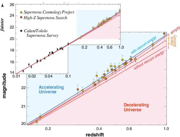
SNIa are thought to be the result of white dwarfs which accrete and explode upon reaching the Chandrasekhar mass limit. This process enable the Supernovae to have a characteristic intrinsic luminosity, which can be standardised empirically: thus, SNIa are potentially independent distance estimators, i.e. standard candles. Other types of Supernovae, instead, have more complex collapsing processes and different intrinsic luminosities, being thus less standardisable. In Fig. 1.6 we show the SNIa observations from the Supernova Cosmology Project and High-Z Supernova Search (high z) and from Calan/Tololo Supernova Survey (Hamuy et al. 1993, 1995) (low

z), on a logarithmic redshift scale. The apparent magnitude of SNIa is proportional to the luminosity distance, which is associated to the redshift of the host galaxy. The measured luminosity distance can be compared to the theoretical prediction (see Eq. 1.27) to constrain Ωm, ΩΛ and discriminate between different cosmological

scenarios. In fact, here the SNIa observations are compared to few cosmological model: data are strongly inconsistent with Λ = 0 models and favour models with Λ > 0 (Perlmutter 2003). While high-redshift SNIa reveal that the Universe is now accelerating (Riess et al. 1998a; Perlmutter et al. 1999), nearby ones provide the most precise measurements of the present expansion rate,H0. The most precise

measurement ofH0 comes from the luminosity calibration of nearby SNe Ia through

Hubble Space Telescope observations of Cepheids in their host galaxies, carried on by the SH0ES program. With this method, Riess et al. (2011) obtained a value of the Hubble constant ofH0 = (73.8±2.4) km s−1Mpc−1 (68% c.l.), including

Figure 1.6: Hubble diagram from SNIa, showing the apparent magnitude on a logarith-mic redshift scale for nearby (Calan/Tololo Supernova Survey) and distant (Supernova Cosmology Project, High-Z Supernova Search) Type Ia Supernovae. At redshifts beyond

z = 0.1, the cosmological predictions start to diverge, depending on the assumed cosmic densities. The red curves represent models with zero vacuum energy and mass densities from the critical density down to zero. The best fit (blue line) assumes a mass density of about ρc/3 plus a vacuum energy density of about 2ρc/3, implying an accelerating cosmic

expansion. Credit: Perlmutter (2003).

1.3.2

Baryon Acoustic Oscillations

Prior to the decoupling phase of the Universe, when photons were scattered by electrons through Thomson scattering, radiation pressure opposed the gravitational collapse of matter, generating pressure waves, known as BAO. These oscillations left a signature in the distribution of matter on very large scales and in the features of CMB anisotropies (Hu & Dodelson 2002). This signature has been measured by galaxy surveys as an overdensity of galaxies at a characteristic comoving scale of 100h−1 _{Mpc. For example, Fig. 1.7 shows the statistically significant bump on this}

1.3 Cosmological probes 21

Figure 1.7: The measured galaxy redshift-space correlation function of the SDSS LRG sample as a function of the comoving separation. The green, red and blue curves represent respectively models with Ωmh2 ={0.12,0.13,0.14}, for fixed Ωbh2 = 0.024 and ns= 0.98.

The magenta line shows a pure CDM model (Ωmh2 = 0.105), with no evidence of an acoustic peak. Credit: Eisenstein et al. (2005).

1.3.3

The Cosmic Microwave Background Radiation

The CMB appears to us as an isotropic radiation filling the whole Universe in all directions, with a characteristic black body spectrum at the temperature of approx-imately TCMB = 2.73K. According to the cosmological principle, the Universe, and

thus the CMB, is approximately isotropic and homogeneous on those large scales. More accurate investigations and more recent measurement, such as the ones by the COBE (Boggess et al. 1992; Smoot et al. 1992), WMAP (Bennett et al. 2013) and Planck (Planck Collaboration et al. 2013a) satellites show the presence of tiny tem-perature irregularities (see Fig. 1.8): these correspond to regions of slightly different densities, which represent the seeds of all structures we see today. More precisely, it has been observed that the distribution of the CMB is isotropic to the precision of 10−3_{: the background (monopole, l = 0) appears completely uniform at a}

tem-perature of 2.73 K. Most of the residual anisotropy is due to the dipole anisotropy (l= 1, ∼mK), caused to the Doppler effect from the motion of the Sun with respect to the background radiation and the primordial anisotropy (l _≥2, _∼µK), due to a scattering effect and a gravitational effect (Sachs-Wolfe effect,Sachs & Wolfe 1967). After subtracting all these contributions (including Milky Way emission visible in the central part of the map), we are left with density fluctuations of

∆T

T =

∆ρm

ρm ≈

10−5 _{. (1.43)}

Note that the equality here between temperature and density fluctuations holds only if perturbations are adiabatic.

1.3 Cosmological probes 23

Figure 1.8: The anisotropies of the CMB as observed by Planck satellite. Cold spots are in blue, while hot are in red. Copyright ESA and the Planck Collaboration.

Wilkinson Microwave Anisotropy Probe

The WMAP1_{is a NASA Explorer mission which collected a huge amount of data, now}

fully analysed to obtain important cosmological achievements. Charles Bennett and the WMAP team won the 2012 Gruber Cosmology Prize because of these published results. The WMAP instrument is composed of cooled microwave radiometers, with 1.4_× 1.6 meter diameter primary reflectors, in five frequency bands (22-90 GHz) to allow the separation of the foreground signals from the CMB. WMAP measures the temperature difference between two points in the sky to an accuracy of 10−6

degree: this means also that systematics have been carefully handled. The main achievement of this project has been the first fine-resolution (0.2 deg) full-sky map of the microwave sky. In addition to this, the inflationary model has been supported, as well as the Gaussian distribution of temperature fluctuations. Furthermore, the following constraints on cosmological parameters have been placed : the age of the Universe is 13.77 billion years old, within a 0.5%; the curvature of space is zero within 0.4%; the Universe contents are baryons (4.6%), dark matter (24.0%) and dark energy (71.4%). In our cosmological analysis, we include the CMB spectra from the WMAP Data Release 7, whose detailed cosmological results have been published by Komatsu et al. (2011). Fig. 1.9 shows the CMB temperature power

Figure 1.9: The 7-year temperature (TT) power spectrum from WMAP. The curve is the CDM model best fit to the 7-year WMAP data: Ωbh2 = 0.02270, Ωch2 = 0.1107,

ΩΛ = 0.738, ns = 0.969. The plotted errors include instrumental noise. The grey band

represents cosmic variance. Credit: Larson et al. (2011).

spectruml(l+ 1)Cl/2πas a function of multipolel (l=π/θ) as measured by WMAP DR7 (Larson et al. 2011). The locations and shapes of the first (l_∼200) and second peak (l ∼500) has been detected with high precision, while the third peak (l∼800) is less constrained. The first peak location corresponds to the size of the sound horizon at the last scattering surface. As we can measure the distance to the last scattering surface, knowing the redshift of the CMB, we can locate a point in the Hubble diagram with very high accuracy, and probe the geometry of the Universe. This method measures the Universe to be spatially flat Ωk ∼ 1. The other peaks

instead represent combinations of Ωr, Ωb, Ωm. The cosmology results of WMAP DR9

1.4 Galaxy Clusters 25

1.4

Galaxy Clusters

Clusters of galaxies are a particularly rich source of information about the underlying cosmological model. They are the largest and most recent collapsed objects in the Universe. Studies of their evolution and properties can place strong constraints on the growth of structures and on the current cosmological paradigm. Here we briefly describe the history of galaxy clusters observations, their main constituents and observables, their formation process and their role as cosmological probes.

1.4.1

History of galaxy clusters observations

Galaxy clusters were discovered quite early in the history of modern astronomy by Messier (1784) and Herschel (1785), independently. The extragalactic nature of these objects was only later confirmed and galaxy clusters were considered as proper physical objects. Their nature was not recognised until the 1930’s, when the dynamical analysis of Zwicky (1937) and Smith (1936) enable the first estimation of their mass. They showed the evidence for much more gravitational material than indicated by the stellar content of the galaxies in the cluster alone, giving the first hint of DM in the Universe. This was later confirmed by measurements of cluster masses using the velocity distribution of the galaxies by means of the Viral Theorem2 _(Rood

1974b,a). Then, the studies on galaxy clusters were extended to several aspects: origin and evolution, dynamical properties, distribution and characterization of the galaxies inside a cluster. Large catalogues of clusters (Abell 1958; Zwicky et al. 1968) based on eye estimates of the number of galaxies per unit solid angle were developed. The first all sky X-ray survey with the Uhuru satellite (Giacconi et al. 1972) confirmed that many clusters were spatially extended X-ray sources. More recently, the discovery of hot high-redshift clusters by Bahcall & Fan (1998) was the first suggestion of a DE component. Finally, last decades experienced the birth of numerous surveys in all wavelengths and an exponential increase of publications on galaxy clusters. More details about these latest scientific results will be covered in Chapter 3.

2_{The Virial Theorem states that, for a stable, self-gravitating, spherical distribution of objects}

of same mass, it holdsEk=−1/2Ep, whereEk is the total kinetic energy of the objects andEpis

1.4.2

Main features, components and observables

Clusters typically have masses of 1013_-1015_M

⊙, sizes of the order of few Mpc, velocity

dispersions of 800-1000 km/s and X-ray luminosities of 1043_-1045 _{erg/s. Clusters of}

galaxies are typically larger than groups and contain about 50 to 1000 members: this limits assign the denomination of rich and poor cluster, respectively. We can also distinguish clusters between regular, which are spherical with a central region of higher density, and irregular ones, which are instead not spherical and without a unique dense central region. Phenomenologically clusters are composed of:

- Galaxies(2-5%), which contain the condensed baryonic matter in the form of stars and cold gas. The typical population is composed of old and passive (red and dead) galaxies, which ended their star formation at z > 2 and which sit on a red-sequence locus in a colour-magnitude diagram.

- Intra-Cluster Medium (ICM) (11-15%), which mainly consists of hydrogen and helium, represents most of the baryonic matter in a highly ionised form and low density (_∼ 10−3_atoms/cm3_{). As a matter of fact, the ICM reaches}

tem-perature of approximately 108_{K to balance the gravitational pull of the DM}

potential well, and emits in the X-ray band. The main X-ray emission pro-cesses from ICM are collisional: thermal Bremsstrahlung (free-free emission), recombination (free-bound emission), line radiation (bound-bound emission). The emissivity of the Bremsstrahlung mechanism is stronger in the densest innermost regions because is proportional to the squared number density of particles.

- Dark Matter Halo(80-87%): it follows a universal distribution known as the Navarro-Frenk-White (NFW) profile (Navarro et al. 1997), which depends on the central density and scale radius (see Section 2.1.2).

- Intra-Cluster light: it is the optical light from stars which are gravitationally bounded to the cluster itself.

1.4 Galaxy Clusters 27

Figure 1.10: Composite image of three views of the galaxy cluster Abell 520. The optical view shows the galaxies bound together by gravitational force. Diffuse, hot gas in between the galaxies emits X-rays: this is shown in red in the Chandra X-ray Observatory image. Gravitational lensing image is representing, instead, the collisionless core of dark matter component in blue. Credit: X-ray: NASA/CXC/UVic./A.Mahdavi et al.; Optical/Lensing: CFHT/UVic./A.Mahdavi et al..

effect is used to detect clusters with no redshift limitation and is quantified by the Compton y-parameter, i.e. the electron pressure integrated along the line of sight l:

y= Z

kBTX(l)

c2_m

e

ne(l)σTdl . (1.44)

Here kB is the Boltzmann constant, TX is the X-ray temperature, me and ne are the electron mass and number density respectively,σT is the Thomson cross-section. More practically, the quantity which is usually measured is the projection on the cluster area dA, namely the integrated Compton parameter YSZ ∝

R

ydA. Finally, strong features are also detected in the gravitational lensing shear field, which gives information about the DM halo (see Section 2.1.3).

1.4.3

Cluster mass proxies

One of the key issues in the study of galaxy clusters is the determination of their true mass. Cluster total masses cannot be directly determined from observation, but instead they have to be deduced from some observational properties, called mass proxies, which correlate with the true mass via the so-called scaling relations. Various mass proxies in different wavelength and associated systematics have been used so far to determine the mass of clusters from observations, via the respective scaling relations and scatter around them. Here we only list the most common ones:

i) the optical richness, i.e. number of red galaxies within R200: N200 (Rozo et al.

2010) - this is the observable throughout all our analysis;

ii) the line-of-sight velocity dispersion: σv, which is related to the total mass as (Longair 2008) M ∝σ2

vRvir, whereRvir is the virialization radius;

iii) the X-ray temperature, bolometric luminosity, gas mass, gas total thermal energy;

iv) the integrated SZ parameter at mm wavelength.

1.4 Galaxy Clusters 29

1.4.4

Formation of galaxy clusters

Formation and evolution of clusters of galaxies trace directly thehierarchical growth

of structures in the Universe. The first objects which start to collapse and virialize, deviating from the Hubble flow, have sub-galactic sizes. Then, these structures merge to originate the galaxies, which analogously can form galaxy clusters by merging. Fluctuations inside a region grow until they balance the local expansion: at this point, the expansion of the region is slowed down till it reaches a maximum radius. Having no more kinetic energy but only gravitational potential energy, the region collapses: baryons fall into the gravitational potential wells produced by the DM and potential energy is converted into kinetic one. This brings the gas to thermalisation, thus producing the hot plasma. When the Virial Theorem condition is satisfied, the dynamical equilibrium is reached. The kinetic energy of the galaxies moving randomly inside the cluster furnishes a pressure which counteracts the gravitational attraction: this gives stability to the cluster.

1.4.5

Clusters as cosmological probes

As in GR the geometry of the Universe is fully described by the total energy content (see Eq. 1.5), one can study the structure of the Universe by testing the geometry by means of probes such as SNIa, BAO and CMB. Alternatively, it is possible to test both the geometry and the structure with different probes and then compare the constraints. Clusters of galaxies are fundamental because they provide both an independent measure of cosmological parameters with different systematics to the CMB, SNIa and BAO, and a probe of the growth of structures. In particular, galaxy clusters are used to test cosmology my measuring their mass function, namely the number density of clusters as a function of their mass and redshift. The precise determination of the mass function and its evolution can place constraints on the energy components of the Universe. As an example, we show in Fig. 1.11 an early result for the cluster mass function obtained by Bahcall & Cen (1992). The optical data are based on richness, velocities and luminosity function of clusters, while the X-ray data refer to the temperature distribution of clusters. Here the observations of optical and X-ray galaxy clusters are compared with expectations from different cosmologies using CDM large-scale (box size of 400h−1_{Mpc) simulations. The}

com-parison shows that the cluster mass function is a powerful discriminant among mod-els: the Ωm= 1 model cannot reproduce the observations for any bias parameter. In

Figure 1.11: Cluster mass function observations of optical and X-ray data, compared with CDM simulations. A model with Ωm = {0.25,0.35} (with or without a

cosmolog-ical constant), appears to match the observations. The Ωm = 1 model, instead, fails in

reproducing data. Credit: Bahcall & Cen (1992).

bias b = {1.0,1.3}, with or without a cosmological constant, appears to fit well the observations. Precise observations of large numbers of clusters have later provided an important tool for understanding better their abundances. The full theoretical derivation, numerical calibration and discussion on the cosmology dependence of the mass function are provided in Section 2.2. In addition to a predicted mass function and a well-determined relation between the true cluster mass and the observable, a cluster experiment needs a large, clean, complete survey with a well-defined selection function. We list the main X-ray, millimetre, weak lensing and optical cluster surveys in Section 3.1. Complementary to the abundances, theclustering of galaxy clusters, i.e. their spatial distribution at z = 0 and its evolution to higher redshifts, contains fundamental information on the underlying matter distribution as well. We give a detailed description of the cluster power spectrum and its cosmology dependence in Section 2.4.

Detailed theoretical modelling of clusters is a complicated astrophysics problem involving a variety of physical phenomena. Useful tools in this regards are numerical

1.5 ΛCDM standard model 31

1.5

Λ

CDM standard model

Several observations over the past decades confirmed that the Universe is experienc-ing a phase of cosmic acceleration, driven by a dark form of energy with negative vacuum pressure. Perlmutter et al. (1999) with SNIa, Allen et al. (2004, 2008) with clusters of galaxies, Eisenstein et al. (2005) with Large-Scale Structure (LSS) and Komatsu et al. (2011) with the CMB, independently confirm the accelerated expan-sion epoch which is currently ongoing. Therefore the concordance Lambda Cold Dark Matter (ΛCDM) cosmological model has been formulated. It affirms that the Universe is composed of:

ˆ ∼5% of ordinary baryonic matter Ωb, mainly made up by hydrogen atoms (∼

75%), Helium atoms (∼25%), while heavier elements are only a tiny fraction;

ˆ ∼ 25% of unknown (dark) form of matter Ωcdm, made up by species of

sub-atomic particles that interact almost only gravitationally (and not electromag-netically) with ordinary matter, being thus totally collisionless;

ˆ ∼ 70% of unknown (dark) form of energy ΩΛ, responsible of the late time

accelerating expansion;

ˆ a radiation component Ωr, which is negligible today, as Ωr/Ωm ≃1/3250.

There are few probes of the existence of the DM component. One is related to the rotation curves of galaxies (see Fig. 1.12 and Freeman 1970) which do not reveal a Keplerian decline (namely the squared velocity is not proportional to the inverse radius), giving evidence of an undetected matter component. Furthermore, the gravitational lensing in galaxy clusters shows a mismatch between the amount of normal matter and the estimated total mass. In addition to this, the evidence of the collisionless nature of dark matter has been observed in few objects (e.g. the ’bullet cluster’ in Markevitch et al. 2004; Clowe et al. 2004). A fundamental property of DM is that it is non-relativistic (i.e. cold): this is necessary to explain the struc-ture formation model currently accepted. Possible candidates for a DM particle are provided by theoretical particle physics, e.g. Weakly Interacting Massive Particles (WIMPSs), which are massive particles interacting through the weak nuclear force and gravity.

Figure 1.12: Rotation curve of galaxy NGC 6503: the data points with error bars are the observed velocities, the disk stars contribution is shown by the dashed line, while the contribution of the gas is represented by the dotted line. As Freeman (1970) first noticed that the expected Keplerian decline (i.e. v2 _∝r−1) was not present in NGC 300 and M33 galaxies, also here there is clear evidence of an undetected dark matter halo component, with densityρDM(r)∝r−2. Credit: Kamionkowski (1998).

the cosmological constant problem appears if we associate Λ to the vacuum energy, i.e. the background energy in absence of matter: the observed cosmological constant is smaller by a factor of _∼10120 _{than the value for the vacuum energy predicted by}

quantum field theories. In addition to this, the coincidence problem asks why we live at the special epoch where DE density is approximately equal to matter density. Numerous alternative theories try to explain the nature of this constituent (e.g. quintessence,...). For example, by assuming that the equation of state of DE evolves in time, we obtainw(z) =w0+w′z (Maor et al. 2001; Weller & Albrecht 2001, 2002),

which diverges at high redshift, or w(z) =w0+w1z/(1 +z) (Chevallier & Polarski

1.5 ΛCDM standard model 33

1.5.1

Cosmological constraints from observations

For completeness, we now list the main cosmological parameters in the concordance ΛCDM model, which govern the global properties of the Universe and the spectrum of the initial density perturbations, together with their current constraints from the latest Planck mission (Planck Collaboration et al. 2013b) (see Table 1.2).

Symbol Definition Constraint

ωb = Ωbh2 Baryon density 0.02214±0.00024

ωcdm = Ωch2 Cold Dark Matter density 0.1187±0.0017

Ωk Spatial curvature -0.0005+0−0..00650066

ΩΛ Dark Energy density 0.692±0.010

ln(1010_A

s) Primordial pert. amplitude 3.091±0.025

σ8 RMS matter fluctuations 0.826±0.012

w Constant EoS of Dark Energy -1.13+0−0..2325

τ Reionization optical depth 0.092_±0.013

ns Primordial scalar spectral index 0.9608±0.0054

P

mν Sum of the neutrino masses in eV <0.230

Neff Effective number of neutrino-like species 3.30+0−0..5451

H0 Hubble constant 67.80±0.77

t0 Age of the Universe (Gyr) 13.798±0.037

zre Redshift of half-reionization 11.3±1.1

100θ∗ _{100 × angular size of sound horizon 1.04162±0.00056}

Table 1.2: List of the main cosmological parameters of ΛCDM model, together the con-straints from Planck+WMAP+highL+BAO (Planck Collaboration et al. 2013b) for the following models: six parameter base ΛCDM model and derived parameters (blue, 68% limits) and extensions to the base ΛCDM model (green, 95% limits).

Ωm−σ8 constraints

Constraints on Ωm−σ8plane were investigated by Mantz et al. (2010) comparing and

combining three Rosita All Sky Surveys (RASS). Independent clusters studies of op-tical clusters (Rozo et al. 2010) (see left panel of Fig. 1.13), Sunyaev-Zeldovich clus-ters in combination with X-ray measurements (Benson et al. 2013) and X-ray clusclus-ters (Vikhlinin et al. 2009) showed consistent results. In the right panel of Fig. 1.13 we show Allen et al. (2008) constraints on the Ωm−ΩΛ plane, from the combination of

Chandra measurements of the X-ray gas mass fraction fgas of galaxy clusters, SNIa

data and CMB measurements.

Neutrinos

As any particle with a non-zero mass transits while cooling from a relativistic state to a non-relativistic state, the mass of neutrinos influences the background evolution and cosmic structure formation. The quantity typically used to describe neutrinos mass is Pmν, which is the species-summed mass. Constraints on this quantity come from clusters combined with CMB data (Burenin & Vikhlinin 2012). Few more considerations on this topic are included in Chapter 6.

Ω

m

Ω Λ

0 0.2 0.4 0.6 0.8 1 0

0.2 0.4 0.6 0.8 1 1.2 1.4 1.6

SNIa

CMB Cluster fgas

Figure 1.13: Left panel: Joint 68.3% and 95.4% confidence regions in the Ωm −σ8

plane from optical galaxy cluster of the maxBCG catalogue combined with WMAP5 (Dunkley et al. 2009). Right panel: contours for Ωm−ΩΛ from the combination of

1.5 ΛCDM standard model 35

DE equation of state

Allen et al. (2011) analysed the constraints on the DE equation of state together with Ωm (see left panel of Fig. 1.14) or σ8. He combined the abundance and

growth of RASS clusters (Mantz et al. 2010),fgas measurements (Allen et al. 2008),

WMAP5 results (Dunkley et al. 2009), Supernovae Ia data (Kowalski et al. 2008) and BAO measurements (Percival et al. 2010, 2011). Constraints on DE equation of state from data were also performed by Rapetti et al. (2005) with X-ray clus-ters+SNIa+CMB, by Mantz et al. (2010); Benson et al. (2013) with X-ray clusters, while Vikhlinin et al. (2009) constrained w and ΩΛ.

Cosmic growth γ

Rapetti et al. (2013) tested the cosmic growth predicted by GR (γ = 0.55) with three independent measurements: galaxy clusters abundances and fgas from RASS

and Chandra, galaxy clustering from WiggleZ Dark Energy Survey, 6-degree Field Galaxy Survey and CMASS BOSS, and CMB from WMAP. The cosmic growth is modelled by the growth index γ defined in Eq. (1.36) and σ8. We show in the right

panel of Fig. 1.14 the constraints obtained on these parameters.

σ8

γ

0.4 0.6 0.8 1 1.2 1.4 1.6 −0.5

0 0.5 1 1.5 2 2.5

CMB cl

gal cl+CMB+gal

Figure 1.14: Left panel: Joint 68.3% and 95.4% confidence regions forw−Ωm, from the

abundance and growth of RASS clusters (violet), X-ray gas mass fraction (pink), WMAP5 (blue), SNIa (green) and BAO (brown). Right panel: joint contours in the σ8−γ plane,