A staggered eigensolver based on sparse matrix
bidiagonalization
James C.Osborn1,and Xiao-YongJin1
1Leadership Computing Facility, Argonne National Laboratory, 9700 S. Cass Ave., Argonne, IL 60439, USA
Abstract.We present a method for calculating eigenvectors of the staggered Dirac op-erator based on the Golub-Kahan-Lanczos bidiagonalization algorithm. Instead of using orthogonalization during the bidiagonalization procedure to increase stability, we choose to stabilize the method by combining it with an outer iteration that refines the approxi-mate eigenvectors obtained from the inner bidiagonalization procedure. We discuss the performance of the current implementation using QEX and compare with other methods.
1 Introduction
We are interested in calculating the eigenvalues and eigenvectors of the staggered Dirac operator. These can be used in a deflated solver, to decrease the number of iterations needed to solve the Dirac equation, and in variance reduction methods for correlator calculations [1–3].
Common eigensolver methods previously used for staggered fermions include nonlinear Conju-gate Gradient [4], Jacobi-Davidson [5], and Lanczos based methods [6]. Here we employ a diff
er-ent method based on finding singular values and vectors of the odd-even staggered hopping matrix A=Doe.
The staggered Dirac matrix has the form
Ds(m)=
m A
−A† m
(1)
If we were to find the singular value decomposition (SVD) of the hopping matrix as
A=QΛW† (2)
whereQandWare unitary matrices of singular vectors, andΛis a diagonal matrix of singular values,
then the eigenvalues ofDs(0) are just±iΛand the eigenvectors are easily obtained fromQandW. The inverse of the Dirac matrix in this basis can be written as
Ds(m)−1=
Q 0
0 W m
Λ
−Λ m
−1 Q
† 0
0 W†
. (3)
Speaker, e-mail: [email protected]Acknowledgments:This research used resources of the Argonne Leadership
Com-puting Facility (ALCF), which is a U.S. Department of Energy Office of Science User Facility operated under Contract
DE-AC02-06CH11357. JCO was supported by the ALCF. XYJ was supported by the U.S. Department of Energy Office of Science
In practice we will not be able to obtain the full SVD ofA, and will instead try to find some set of vectors that approximate the lowest singular modes ofA,
AW˜ ≈Q˜Λn (4)
where ˜Wand ˜Qare matrices withnorthogonal columns andΛnis the diagonal matrix of thensmallest singular values of A. We can still use the form (3) to approximate the inverse by replacing the matrices from the full SVD with their approximate lower-rank versions. As mentioned above, this can be used in a deflated solver and in improved operators for correlator measurements. Note that in the end we only need to keep track of the vectors in ˜Wsince ˜Qcan easily be reconstructed from eq. (4).
The motivation for using an SVD algorithm is mainly that of stability. An alternative would be to use an eigenvalue algorithm on the normal form,A†A. For a matrix with a small condition number,
this may work well, but for larger condition numbers it will become more difficult since the condition
number of the normal form is the square of the condition number ofA.
Another alternative is to apply an Hermitian eigensolver to the Jordan-Wielandt form
0 A
A† 0
(5)
which is, up to a sign, the same as the massless staggered Dirac matrix. This is expected to be more stable whenAis ill-conditioned. Applying Lanczos tridiagonalization to this matrix, for a particular starting vector, is equivalent to applying the Golub-Kahan-Lanczos (GKL) bidiagonalization proce-dure to the matrixA. Here we adopt the GKL method to calculate an approximation to the smallest singular values ofAalong with their corresponding vectors.
Afterksteps of the Golub-Kahan-Lanczos bidiagonalization procedure [7] in exact arithmetic, we have
AVk = UkBk (6)
A†U
k = VkB†k+βkvk+1e†k (7)
whereVkandUKare matrices containingkorthonormal columns each (with columns denoted asvi andui),ekis a lengthkvector with 1 in elementkand the rest zeros,αiandβiare real valued, and
Bk=
α1 β1
α2 . ..
. .. βk−1
αk
. (8)
This is calculated by an iterative process, starting with an initial vectorv1, then generatingα1 and u1 using equation (6), then gettingβ1andv2from equation (7), and repeating for increasingk. An example of the code for this method is in the Appendix.
If we calculate the SVD of the bidiagonal matrixBk(which can be done cheaply using standard Lapack routines)
BkXk=YkΛk (9)
whereXkandYkare dimensionkunitary matrices, andΛkis a diagonal matrix of singular values, we can then write
In practice we will not be able to obtain the full SVD ofA, and will instead try to find some set of vectors that approximate the lowest singular modes ofA,
AW˜ ≈Q˜Λn (4)
where ˜Wand ˜Qare matrices withnorthogonal columns andΛnis the diagonal matrix of thensmallest singular values of A. We can still use the form (3) to approximate the inverse by replacing the matrices from the full SVD with their approximate lower-rank versions. As mentioned above, this can be used in a deflated solver and in improved operators for correlator measurements. Note that in the end we only need to keep track of the vectors in ˜Wsince ˜Qcan easily be reconstructed from eq. (4).
The motivation for using an SVD algorithm is mainly that of stability. An alternative would be to use an eigenvalue algorithm on the normal form,A†A. For a matrix with a small condition number,
this may work well, but for larger condition numbers it will become more difficult since the condition
number of the normal form is the square of the condition number ofA.
Another alternative is to apply an Hermitian eigensolver to the Jordan-Wielandt form
0 A
A† 0
(5)
which is, up to a sign, the same as the massless staggered Dirac matrix. This is expected to be more stable whenAis ill-conditioned. Applying Lanczos tridiagonalization to this matrix, for a particular starting vector, is equivalent to applying the Golub-Kahan-Lanczos (GKL) bidiagonalization proce-dure to the matrixA. Here we adopt the GKL method to calculate an approximation to the smallest singular values ofAalong with their corresponding vectors.
Afterksteps of the Golub-Kahan-Lanczos bidiagonalization procedure [7] in exact arithmetic, we have
AVk = UkBk (6)
A†U
k = VkB†k+βkvk+1e†k (7)
whereVkandUK are matrices containingkorthonormal columns each (with columns denoted asvi andui),ekis a lengthkvector with 1 in elementkand the rest zeros,αiandβiare real valued, and
Bk=
α1 β1
α2 . ..
. .. βk−1
αk
. (8)
This is calculated by an iterative process, starting with an initial vectorv1, then generatingα1 and u1 using equation (6), then gettingβ1 andv2 from equation (7), and repeating for increasingk. An example of the code for this method is in the Appendix.
If we calculate the SVD of the bidiagonal matrixBk(which can be done cheaply using standard Lapack routines)
BkXk=YkΛk (9)
whereXkandYkare dimensionkunitary matrices, andΛkis a diagonal matrix of singular values, we can then write
AWk=QkΛk (10)
withWk=VkXKandQk=UkYk.
If this process is continued in exact arithmetic forNsteps, whereNis the dimension ofA, then equation (10) would give the full SVD of A. For anyk < N, equation (10) would not give the full SVD of A, and the values ofΛkwould only approximate some of the singular values of A.
In finite precision the iterative process will not produce orthogonal column vectors inVk and Uk. This can be remedied by either a full or selective reorthogonalization. Even in the selective case, this can be relatively expensive. In our tests we have run the GKL process for over 10,000 iterations, so the cost of trying to keep them orthogonal can become large. Also we are currently only interested in keeping the lowest O(1,000) eigenvectors, so there is no need to keep all of the GKL vectors orthogonal. We therefore choose to fix the orthogonality after the approximate SVD with a Rayleigh-Ritz update by solving the generalized eigenproblem
(W†A†AW)Z=(W†W)ZE (11)
forZ, then computing the refined singular vectors as
W=WZ. (12)
For large enoughk, the combination of using the GKL-based method to produce a large number of approximate singular vectors, along with the final Rayleigh-Ritz procedure to refine the lowest vectors and ensure orthogonality, will produce a good set of low modes of the staggered Dirac matrix suitable for deflation or variance reduction.
2 Implementation
This method for calculating low eigenvectors of the staggered Dirac operator was originally imple-mented around 2011 using Qlua [8] and QOPQDP [9]. Since it was being used to study eigen-value/vector statistics and for deflation it was designed to achieve high precision, especially for
near-zero eigenmodes. That code adopted an iterative approach which repeated the GKL based approxi-mate SVD and Rayleigh-Ritz procedures until some convergence criteria were achieved. The basic method outline is
W1 = GKLanczosSVD( randomVector ) repeat until converged:
x = smallestUnconverged( W1 ) W2 = GKLanczosSVD( x )
W1 = combine(W1, W2)
HereGKLanczosSVDis the GKL based approximate SVD described above which is given an initial vector, and returns a set of approximate singular vectors. Convergence is determined by checking the norm of the residual
ri=A†Awi−λ2iwi (13)
which places a bound on the accuracy of the corresponding eigenvalue
error(λ2i)≤ |ri|. (14)
We allow both an absolute (σabs) and relative (σrel) convergence bound for the eigenvalues, determined by
After checking if enough singular values have converged,smallestUnconvergedreturns the vector corresponding to the smallest approximate singular value that hasn’t converged yet, which is used to start a new GKL process. Repeating this procedure then ensures that the lowest eigenvectors will eventually converge.
Most of the algorithmic design choices went into thecombineprocedure above. Ideally it would do a full diagonalization ofA†Ain the span of W1 and W2, however this can be expensive. Instead
the full diagonalization can be approximated with many smaller ones by diagonalizing over spaces of vectors with similar approximate eigenvalues. There are many ways to do this and the details can make big difference in convergence properties. We will not discuss the details here due to lack of
space.
We recently ported the old code to a new framework, QEX (Quantum Expressions) [10–12]. This is a new lattice field theory framework written in the Nim[13] programming language (see the contri-bution to this conference [14]). Nim has a python-like syntax, though is strongly typed and compiles to C/C++code making it efficient and portable. Converting the Lua code to Nim was fairly easy to
do by hand (Lua dynamic types can be written as Nim generics). Converting the underlying C code to Nim was done with the c2nim[15] tool plus some cleanup by hand.
After the initial port, we worked on tuning the code and improving the method. The current version of the code scales well to over 100,000 iterations. This allowed us to experiment with generating eigenvectors from a single large GKL run. This is not necessarily the most efficient way to use it, but
we wanted to see how many iterations were needed for the method to converge to the lowest singular vector without any restarts.
3 Results
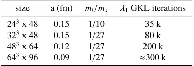
Table 1: MILC HISQ ensembles used for testing.
size a (fm) ml/ms λ1GKL iterations
243x 48 0.15 1/10 35 k
323x 48 0.15 1/27 80 k
483x 64 0.12 1/27 200 k
643x 96 0.09 1/27 ≈300 k
We performed some tests of the algorithm using some MILC HISQ ensembles [16] on a Blue Gene/Q supercomputer. In table1we list the relevant parameters of the ensembles used along with
the number of GKL iterations that were needed for the lowest singular value (λ1) to converge using
σrel=10−6andσabs=10−8. Once the lowest singular value has converged, many more low ones will have converged too. The results are from only one configuration from each ensemble, however we have run on a few other configurations from thea≈0.15 fm ensembles and found similar results.
The number of iterations needed grows with the lattice volume (though not quite as fast as linear in volume). The large number of iterations needed makes it prohibitive to store all the vectors from the GKL process, so we instead make two passes: first calculating the matrixBk, then we can find the matrixXkand do a second GKL pass accumulating the vectors ofWkas it goes.
In order to cross check results and compare performance, we used the eigensolver provided in PRIMME [5] on the normal form, A†A. We created a Nim wrapper [17] for the C interface of
After checking if enough singular values have converged,smallestUnconvergedreturns the vector corresponding to the smallest approximate singular value that hasn’t converged yet, which is used to start a new GKL process. Repeating this procedure then ensures that the lowest eigenvectors will eventually converge.
Most of the algorithmic design choices went into thecombineprocedure above. Ideally it would do a full diagonalization ofA†Ain the span of W1 and W2, however this can be expensive. Instead
the full diagonalization can be approximated with many smaller ones by diagonalizing over spaces of vectors with similar approximate eigenvalues. There are many ways to do this and the details can make big difference in convergence properties. We will not discuss the details here due to lack of
space.
We recently ported the old code to a new framework, QEX (Quantum Expressions) [10–12]. This is a new lattice field theory framework written in the Nim[13] programming language (see the contri-bution to this conference [14]). Nim has a python-like syntax, though is strongly typed and compiles to C/C++code making it efficient and portable. Converting the Lua code to Nim was fairly easy to
do by hand (Lua dynamic types can be written as Nim generics). Converting the underlying C code to Nim was done with the c2nim[15] tool plus some cleanup by hand.
After the initial port, we worked on tuning the code and improving the method. The current version of the code scales well to over 100,000 iterations. This allowed us to experiment with generating eigenvectors from a single large GKL run. This is not necessarily the most efficient way to use it, but
we wanted to see how many iterations were needed for the method to converge to the lowest singular vector without any restarts.
3 Results
Table 1: MILC HISQ ensembles used for testing.
size a (fm) ml/ms λ1GKL iterations
243x 48 0.15 1/10 35 k
323x 48 0.15 1/27 80 k
483x 64 0.12 1/27 200 k
643x 96 0.09 1/27 ≈300 k
We performed some tests of the algorithm using some MILC HISQ ensembles [16] on a Blue Gene/Q supercomputer. In table1we list the relevant parameters of the ensembles used along with
the number of GKL iterations that were needed for the lowest singular value (λ1) to converge using
σrel=10−6andσabs=10−8. Once the lowest singular value has converged, many more low ones will have converged too. The results are from only one configuration from each ensemble, however we have run on a few other configurations from thea≈0.15 fm ensembles and found similar results.
The number of iterations needed grows with the lattice volume (though not quite as fast as linear in volume). The large number of iterations needed makes it prohibitive to store all the vectors from the GKL process, so we instead make two passes: first calculating the matrixBk, then we can find the matrixXkand do a second GKL pass accumulating the vectors ofWkas it goes.
In order to cross check results and compare performance, we used the eigensolver provided in PRIMME [5] on the normal form, A†A. We created a Nim wrapper [17] for the C interface of
PRIMME, plugged it into QEX, and tested on two lattice volumes, 243×48 and 323×48. We found
that using the SVD solver in PRIMME onAdirectly provided no advantage over its eigensolver on A†Afor our purposes, so we focused on using its eigensolver. We introduced a custom convergence
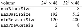
test to the PRIMME eigensolver to implement the convergence criteria in (15). Our inexhaustive tun-ing of PRIMME parameters provided about a 3 times speedup over the default parameters, and for the following tests, we settled on using the preset method ofPRIMME_DEFAULT_MIN_TIME, paired with settings:
volume 243×48 323×48
maxBlockSize 8 8
maxBasisSize 192 512
minRestartSize 120 400
maxPrevRetain 2 8
In order to compare the quality of the converged eigenvectors between different methods, we use
their effectiveness at deflation as a measure. For this we compare the number of conjugate gradient
(CG) iterations needed to solve forxin the linear systemDsx=bto within a residual of 10−8, where the vectorbis projected out of the space spanned by the eigenvectors corresponding to the smallest singular values. By removing the low eigenmodes ofDs fromb, the effective condition number of Ds decreases, and so does the number of CG iterations. The quality of the eigenvectors associates directly with the subtraction of low eigenmodes fromb. Therefore, the number of CG iterations for the deflated vectorbindicates the quality of the eigenvectors.
As an initial test to determine the appropriate convergence criteria, we study the effect of the
convergence criteria on the deflated solver. Here we just use results from the PRIMME eigensolver. Figure1shows the effect of the residual constraint from our convergence test on deflation. It shows the
number of conjugate gradient iterations required for solving against a vector deflated by the generated eigenvectors corresponding to the lowest eigenvalues. We have requested 600 and 400 eigenvectors corresponding to the lowest eigenvalues respectively for the volumes of 243×48 and 323×48. The looser convergence condition degrades the deflation for larger numbers of eigenvectors, which shows in the figure as lines departing from the one with the lowest number of iterations, which usesσrel =
10−6 andσabs =10−8. The zigzag feature of the lines of the degraded deflation is likely an artifact from the block algorithm used in PRIMME.
0 500 1000 1500 2000 2500 3000 3500
0 100 200 300 400 500 600
CG
iterations
number of deflated eigenvectors 𝜎𝜎rel= 10−4,𝜎𝜎abs= 10−6 𝜎𝜎rel= 10−5,𝜎𝜎abs= 10−7 𝜎𝜎rel= 10−6,𝜎𝜎abs= 10−8
(a) 243×48
0 1000 2000 3000 4000 5000 6000 7000 8000
0 50 100 150 200 250 300 350 400
CG
iterations
number of deflated eigenvectors 𝜎𝜎rel= 10−4,𝜎𝜎abs= 10−6 𝜎𝜎rel= 10−5,𝜎𝜎abs= 10−7 𝜎𝜎rel= 10−6,𝜎𝜎abs= 10−8
(b) 323×48
Figure 1: Effect of residual on deflation generated with PRIMME on two lattice volumes, 243×48 (a)
0 0.2 0.4 0.6 0.8 1
0 20 40 60 80 100 120 140 160 180
de
flat
ed C
G it
er
at
ions / nonde
flat
ed C
G it
er
at
ions
cost of eigensolver (in nondeflated solves) PRIMME 100 vectors PRIMME 200 vectors PRIMME 300 vectors PRIMME 400 vectors PRIMME 500 vectors PRIMME 600 vectors 100 vectors 200 vectors 300 vectors 400 vectors 500 vectors 600 vectors
Figure 2: Deflated iterations vs. eigensolver cost (243×48)
0 0.2 0.4 0.6 0.8 1
0 20 40 60 80 100 120
de
fl
at
ed C
G it
er
at
ions / nonde
fl
at
ed C
G it
er
at
ions
cost of eigensolver (in nondeflated solves) PRIMME 200 vectors PRIMME 400 vectors 100 vectors 200 vectors 300 vectors 400 vectors 500 vectors 600 vectors
Figure 3: Deflated iterations vs. eigensolver cost (323×48)
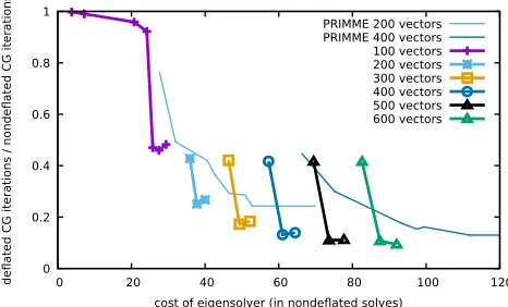
Last we look at the quality of eigenvectors, as measured by deflation, versus their respective costs to generate. Figures2,3, and4show the results for three lattice volumes, 243×48, 323×48, and 483 ×64. The vertical axis indicates the number of CG iterations required for the deflated source vector normalized by the number of CG iterations required for the nondeflated vector. The horizontal axis is the cost of the eigensolver divided by the cost of one nondeflated CG solve. The thicker lines with symbols are from the method presented here while the thinner lines are from PRIMME. In both cases we have given results from several different numbers of approximate eigenvectors generated
which are then used for deflation.
0 0.2 0.4 0.6 0.8 1
0 20 40 60 80 100 120 140 160 180
de flat ed C G it er at
ions / nonde
flat ed C G it er at ions
cost of eigensolver (in nondeflated solves) PRIMME 100 vectors PRIMME 200 vectors PRIMME 300 vectors PRIMME 400 vectors PRIMME 500 vectors PRIMME 600 vectors 100 vectors 200 vectors 300 vectors 400 vectors 500 vectors 600 vectors
Figure 2: Deflated iterations vs. eigensolver cost (243×48)
0 0.2 0.4 0.6 0.8 1
0 20 40 60 80 100 120
de fl at ed C G it er at
ions / nonde
fl at ed C G it er at ions
cost of eigensolver (in nondeflated solves) PRIMME 200 vectors PRIMME 400 vectors 100 vectors 200 vectors 300 vectors 400 vectors 500 vectors 600 vectors
Figure 3: Deflated iterations vs. eigensolver cost (323×48)
Last we look at the quality of eigenvectors, as measured by deflation, versus their respective costs to generate. Figures2,3, and4show the results for three lattice volumes, 243×48, 323×48, and 483×64. The vertical axis indicates the number of CG iterations required for the deflated source vector normalized by the number of CG iterations required for the nondeflated vector. The horizontal axis is the cost of the eigensolver divided by the cost of one nondeflated CG solve. The thicker lines with symbols are from the method presented here while the thinner lines are from PRIMME. In both cases we have given results from several different numbers of approximate eigenvectors generated
which are then used for deflation.
For the GKL based eigensolver (those not labeled ‘PRIMME’ in the figure) each line represents varying numbers of total GKL iterations performed. When the number of iterations is small, the small-est eigenvector does not converge well, and the number of deflated CG iterations is large, indicating poor quality of eigenvectors. The quick dip to the minimum is realized when the GKL iterations is just enough for the smallest eigenvector to converge. This corresponds (approximately) to the number of iterations given in table1. Setting too many GKL iterations, however, introduces duplicate copies
0 0.2 0.4 0.6 0.8 1
0 20 40 60 80 100 120 140
de flat ed C G it er at
ions / nonde
flat ed C G it er at ions
cost of eigensolver (in nondeflated solves) 100 vectors 200 vectors 300 vectors 400 vectors
Figure 4: Deflated iterations vs. eigensolver cost (483×64)
of the eigenvectors, and effectively reduces the span of the low eigenmodes, which in turn increases
the number of deflated CG iterations above the optimum value.
For the 323×48 ensemble we find that deflation can give between a 6×to 10×reduction in the number of CG iterations for a range of 300 to 600 vectors. The setup cost of generating the vectors varies from around 50 to 90 nondeflated CG solves. This means that if one is performing a much larger number of solves than this on a particular configuration, it is beneficial to calculate and deflate eigenvectors. On the 483×64 ensemble, we find about a 4×reduction in CG iterations using 400 vectors at a cost of about 110 nondeflated solves.
The results from PRIMME are obtained by varying the convergence criteria. The looser the con-vergence condition, the quicker it generates the eigenvectors, and the larger the number of deflated CG iterations due to poorer eigenvectors. The best results for each number of vectors are connected together to form a line just for convenience in presentation. In all cases we see that the GKL based eigensolver produces higher quality vectors at a fixed cost. We note that neither method may be tuned optimally, so the comparison is not an absolute statement about the efficiency of either method, but
shows that the new GKL based method is clearly competative with other established methods.
4 Summary
We have presented a method for calculating singular values and their corresponding vectors of a large sparse matrix based on the Golub-Kahan-Lanczos bidiagonalization process. This method was applied to the odd-even hopping matrix of the staggered Dirac operator which can then be used to calculate eigenvalues and eigenvectors of the Dirac operator.
We have found that the method achieves good efficiency in calculating eigenvectors on up to a
483 ×64 HISQ lattice, and have had some preliminary success on a 643×96 lattice. The method provides accurate eigenvectors which are suitable for use in deflation methods to speed up the time to solution for CG. In our tests we found that the deflated solver achieves up to a 10×reduction in CG iterations on a 323×48 lattice (using 600 vectors), and at least a 4×reduction in iterations for a 483×64 lattice (using 400 vectors).
We are currently investigating methods to quickly regenerate the deflation vectors from storing only a reduced number of vectors. This would allow one to efficiently save the deflation vectors for
5 Appendix
Here is an example of the main GKL bidiagonalization loop written in QEX.
var beta = 1.0 var k = 0
p := src / sqrt(src.norm2) u := 0
while true: v := p / beta linop.apply(r, v) r -= beta*u
let alpha = sqrt(r.norm2) a[k] = alpha
inc k
if k >= kmax: break
u := r / alpha linop.applyAdj(p, u) p -= alpha*v
beta = sqrt(p.norm2) b[k-1] = beta
References
[1] H. Neff, N. Eicker, T. Lippert, J.W. Negele, K. Schilling, Phys. Rev. D64, 114509 (2001), hep-lat/0106016
[2] T.A. DeGrand, S. Schaefer, Comput. Phys. Commun.159, 185 (2004),hep-lat/0401011
[3] L. Giusti, P. Hernandez, M. Laine, P. Weisz, H. Wittig, JHEP04, 013 (2004),hep-lat/0402002
[4] T. Kalkreuter, H. Simma, Comput. Phys. Commun.93, 33 (1996),hep-lat/9507023
[5] A. Stathopoulos, J.R. McCombs, ACM Transactions on Mathematical Software37, 21:1 (2010),
http://www.cs.wm.edu/~andreas/software
[6] A. Stathopoulos, K. Orginos, SIAM J. Sci. Comput.32, 439 (2010),0707.0131
[7] G.H. Golub, W.M. Kahan, SIAM J. Num. Anal.Ser. B, 205 (1965) [8] https://usqcd.lns.mit.edu/redmine/projects/qlua
[9] https://github.com/usqcd-software/qopqdp
[10] X.Y. Jin, J.C. Osborn, PoSICHEP2016, 187 (2016),1612.02750
[11] J. Osborn, X.Y. Jin, PoSLATTICE2016, 271 (2017) [12] https://github.com/jcosborn/qex
[13] https://nim-lang.org
[14] https://makondo.ugr.es/event/0/session/102/contribution/407
[15] https://github.com/nim-lang/c2nim
[16] A. Bazavov et al. (MILC), Phys. Rev.D87, 054505 (2013),1212.4768