Loop equation in Lattice gauge theories and bootstrap methods
PeterAnderson1,2,and MartinKruczenski1, 1Department of Physics and Astronomy, Purdue U.,
525 Northwestern Avenue, W. Lafayette, IN 47907-2036, USA. 2Wigner Research Center for Physics of the HAS,
29–33 Konkoly–Thege Miklós Str. H-1121 Budapest, Hungary.
Abstract.In principle the loop equation provides a complete formulation of a gauge the-ory purely in terms of Wilson loops. In the case of lattice gauge theories the loop equation is a well defined equation for a discrete set of quantities and can be easily solved at strong coupling either numerically or by series expansion. At weak coupling, however, we ar-gue that the equations are not well defined unless a certain set of positivity constraints is imposed. Using semi-definite programming we show numerically that, for a pure Yang Mills theory in two, three and four dimensions, these constraints lead to good results for the mean value of the energy at weak coupling. Further, the positivity constraints imply the existence of a positive definite matrix whose entries are expectation values of Wilson loops. This matrix allows us to define a certain entropy associated with the Wilson loops. We compute this entropy numerically and describe some of its properties. Finally we discuss some preliminary ideas for extending the results to supersymmetricN=4 SYM.
1 Introduction
The AdS/CFT correspondence [1–3] motivates the study of gauge theories purely in terms of gauge
invariant operators. In particular, it should be possible to formulate gauge theories in terms of Wilson loops, without reference to the usual Yang-Mills action or any other quantity that is defined in terms of gauge fields or other gauge-dependent variables. One possibility is to have an effective action written
purely in terms of Wilson loop expectation values. It is not known how to do this in a simple way (see [4,5] however). The other possibility is to write equations of motion for Wilson loop expectation values. Those are relatively simple and known as the Migdal-Makeenko loop equations or simply loop equations. The simplest case where one can discuss this problem is in lattice gauge theories since the lattice provides a regularization,i.e. Wilson loops are finite and at the same time the set of Wilson loops is discrete. In the rest of the talk we concentrate in the large-N limit where only single loops, namely single trace operators, need to be considered.
2 Lattice gauge theory
The lattice gauge theory we consider is a simple cubic lattice (see fig.1) with the standard Wilson action:
S =−N 2λ
P
TrUP, (1)
where the sum is over all plaquettes. The gauge group isS U(N) and, as mentioned, we are interested in the large-Nlimit [6,7] whereN→ ∞,gY M →0 keeping the ’t Hooft couplingλ=g2Y MNfixed.
Figure 1.Simple cubic lattice with a plaquette (black) and a random Wilson loop (red) highlighted.
3 Loop equation
We are interested in computing the expectation value of Wilson loops. We start by making a list of loops as illustrated in fig.2. The expectation value of loop jis denoted asWj. The loop equation is
2 Lattice gauge theory
The lattice gauge theory we consider is a simple cubic lattice (see fig.1) with the standard Wilson action:
S =−N 2λ
P
TrUP, (1)
where the sum is over all plaquettes. The gauge group isS U(N) and, as mentioned, we are interested in the large-Nlimit [6,7] whereN→ ∞,gY M→0 keeping the ’t Hooft couplingλ=g2Y MNfixed.
Figure 1.Simple cubic lattice with a plaquette (black) and a random Wilson loop (red) highlighted.
3 Loop equation
We are interested in computing the expectation value of Wilson loops. We start by making a list of loops as illustrated in fig.2. The expectation value of loop jis denoted asWj. The loop equation is
Figure 2.Up to symmetries, Wilson loops of various shapes can be listed as illustrated in the figure
an equation for theWjs derived as a type of Schwinger–Dyson equation in [8]. See also [9–11] for the lattice version that we use here. It has the form
Ki→jWj+2λWi+2λCi→jkWjWk=δi1, (2)
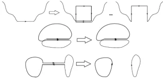
where the matrixKi→jis the so-called loop laplacian that is illustrated graphically in fig.3andCi→jk is the self intersection term whose action is described in the same figure3. The problem with solving
Figure 3.The loop equation contains two non-trivial terms, one is the matrixKthat represents the operation of replacing a link by connecting it to a plaquette with both orientations as illustrated in the first picture, thenCthat represents a self-intersection that splits the Wilson loop in two as illustrated in the two bottom pictures.
the loop equation is easy to understand. To define the problem correctly, either mathematically or numerically, we have to truncate the set of loops to a finite number and eventually let that number go to infinity. For example, we can consider loops of length up to a givenLmax. However, the loop equation for a loop of lengthLinvolves loops of lengthL+4. Therefore we can then only impose the loop equation for loops of length up toLmax−4, namely we have many more loops than equations implying that there is an infinite number of solutions. If we increaseLmaxthis problem persists and we cannot find a unique limit asLmax→ ∞. One possibility is to impose all equations up to lengthLmaxby making a guess for the missing loops of lengthLmax+2 andLmax+4, for example set them to zero but that only works at strong coupling. This was already checked in [12,13]. The alternative procedure we propose [14] is to impose a set of positivity constraints, that we derive in the next section, and that put bounds on the possible solutions that are allowed. In particular we get upper and lower bounds on the expectation value of the plaquette that converge smoothly as we increase the length of the loops, since adding constraints can only lower the upper bound and increase the lower one. Related ideas were discussed previously in [15,16] in the Hamiltonian approach to lattice gauge theory.
4 Positivity constraints
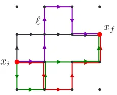
The positivity constraints [14] are derived by considering two points in the lattice and a set of open paths connecting them as in figure4. For a given lattice configuration, to each open pathwe associate
anS U(N) matrixU()as the product of the matrices in each link in the path. Constructing the linear combination
A=
cU() (3)
for arbitrary coefficientscand using that
Tr(A†A)≥0 ⇒
c∗
cTr
(U())†U()
≥0 ⇒
c∗
cTr
(U())†U()
we find that the matrix
ρ=Tr
(U())†U() 0 (5)
is positive definite. Imposing the positivity of this matrix put bounds on the solutions of the loop equation we are allowed to consider. The more open loops we take, the stricter the bounds. Notice that all bounds are exact since we do not use an approximation for the bounds. The approximation is that we do not impose all constraints associated with all possibleρmatrices. The matrixρcan be interpreted as a reduced density matrix where we trace over the color indices. The entropy associated withρdetermines how much information is lost in such tracing. It naively seems to depend on the
choice ofρnamely the choice of initial and final points and on the set of open loops between them as
in fig. 4. In figure5we show that this is not actually the case, in fact for very differentρmatrices,
the entropy is the same up to a small error. We emphasize that this entropy is an entropy computed directly from the Wilson loops and can be defined off-shell, namely for arbitrary values of the Wilson loops, as long as theρmatrix is positive definite.
Figure 4.To construct theρmatrix one chooses two points in the lattice and a set of open loops connecting them.
Figure 5.Different choices ofρmatrices labeled by their final point (the initial point is always 0, give rise to the same entropy implying that the entropy is a well defined quantity related to the lattice theory.)
5 Examples
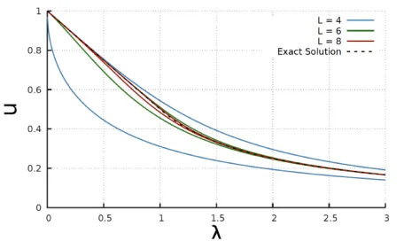
5.1 2D caseThe 2D case was solved exactly by Gross,Witten[17] and Wadia [18]. Here it is just used as a check of the procedure. The results for the expectation value of the plaquette is
W1=u=
1−λ
2 λ≤1
1
2λ λ≥1
(6)
Solving the loop equation and imposing the constraints gives rise to the upper and lower bounds shown in figure6. The numbersLindicate that we keep loops up to length 4L.
Figure 6.Expectation value of the plaquette as a function of ’t Hooft coupling. The exact solution and upper and lower bounds are displayed. The bounds bracket, and quickly converge to the exact solution.
5.2 3D and 4D case
This case is computationally more challenging. The bounds are given in fig.7. We see that, at small coupling, the expectation value for the plaquette agrees well with the upper bound allowed by the positivity constraints and the loop equations. The bounds are not as strict as in 2D since the largest length we consider is 4LwithL=5 instead ofL=8 as in 2D.
6
N
=
4
, bosonic sector, fermions, BPS loops
TheN = 4 theory action can be written in terms of Wilson loops [19–24] and therefore the loop equation can be similarly derived. We tested the bosonic sector of the theory where the action is shown in fig. 8. The loop equation for the plaquette is given in fig.9. Using a numerical simulation we checked the validity of the equations. When including fermions we checked the existence of BPS Wilson loops, namely loops invariant under supersymmetry whose expectation value isW=1. They are constructed out of ¯Uand ¯U−1as illustrated in figure10. HereU=eiA+ΦwhereAis the gauge field
(a) Three dimensions. (b) Four dimensions
Figure 7. The same as the previous figure but for 3D and 4D. In this case the weak coupling solution clearly matches the upper bound showing that the correct solution saturates the bounds at weak coupling
Figure 8.Bosonic part of the action forN=4 in terms of Wilson loops
Figure 9.Loop equation for the plaquette in the bosonic sector ofN=4
Figure 10.BPS loops in latticeN=4 where one supersymmetryQis unbroken
References
[1] J.M. Maldacena, Int. J. Theor. Phys.38, 1113 (1999), [Adv. Theor. Math. Phys.2,231(1998)], hep-th/9711200
[2] S.S. Gubser, I.R. Klebanov, A.M. Polyakov, Phys. Lett.B428, 105 (1998),hep-th/9802109 [3] E. Witten, Adv. Theor. Math. Phys.2, 253 (1998),hep-th/9802150
[4] A. Jevicki, B. Sakita, Nucl. Phys.B165, 511 (1980) [5] L.G. Yaffe, Rev. Mod. Phys.54, 407 (1982) [6] G. ’t Hooft, Nucl. Phys.B72, 461 (1974) [7] G. ’t Hooft, Nucl. Phys.B75, 461 (1974)
[8] Yu.M. Makeenko, A.A. Migdal, Phys. Lett. 88B, 135 (1979), [Erratum: Phys. Lett.89B,437(1980)]
[9] S.R. Wadia, Phys. Rev.D24, 970 (1981) [10] A.M. Polyakov, Nucl. Phys.B164, 171 (1980) [11] T. Eguchi, Phys. Lett.87B, 91 (1979)
[12] G. Marchesini, Nucl. Phys.B239, 135 (1984)
[13] G. Marchesini, E. Onofri, Nucl. Phys.B249, 225 (1985)
[14] P.D. Anderson, M. Kruczenski, Nucl. Phys.B921, 702 (2017),1612.08140 [15] A. Jevicki, O. Karim, J.P. Rodrigues, H. Levine, Nucl. Phys.B230, 299 (1984) [16] A. Jevicki, B. Sakita, Phys. Rev.D22, 467 (1980)
[17] D.J. Gross, E. Witten, Phys. Rev.D21, 446 (1980) [18] S.R. Wadia (2012),1212.2906
[19] S. Catterall, D.B. Kaplan, M. Unsal, Phys. Rept.484, 71 (2009),0903.4881
[20] S. Catterall, D. Schaich, P.H. Damgaard, T. DeGrand, J. Giedt, Phys. Rev.D90, 065013 (2014), 1405.0644
[21] D.B. Kaplan, M. Unsal, JHEP09, 042 (2005),hep-lat/0503039 [22] S. Catterall, J. Giedt, A. Joseph, JHEP10, 166 (2013),1306.3891