The effect of the Polyakov loop on the chiral phase transition
G. Mark´o1,aand Zs. Sz´ep2,b
1 Department of Atomic Physics, E¨otv¨os University, H-1117 Budapest, Hungary
2 Centre de Physique Th´eorique, Ecole Polytechnique, CNRS, 91128 Palaiseau Cedex, France
Abstract. The Polyakov loop is included in the S U(2)L×S U(2)Rchiral quark-meson model by considering the propagation of the constituent quarks, coupled to the (σ,π) meson multiplet, on the homogeneous background of a temporal gauge field, diagonal in color space. The model is solved at finite temperature and quark baryon chemical potential both in the chiral limit and for the physical value of the pion mass by using an expansion in the number of flavors Nf.Keeping the fermion propagator at its tree-level, a resummation on the pion propagator is constructed which resums infinitely many orders in 1/Nf,whereO(1/Nf) represents the order at which the fermions start to contribute in the pion propagator. The influence of the Polyakov loop on the tricritical or the critical point in theµq−T phase diagram is studied for various forms of the Polyakov loop potential.
1 Introduction
The low-energy effective models of the QCD, such as the
Nambu–Jona-Lasinio (NJL) model and the chiral quark-meson model (QM), are based on the global chiral sym-metry of the QCD. They are very useful to qualitatively understand many aspects related to the spontaneous break-ing of the chiral symmetry and its restoration at finite tem-perature and density. However, the absence of gluonic ef-fective degrees of freedom and the lack of color clustering alter the reliability of the quantitative thermodynamic pre-dictions of these models, such as the equation of state or the location of the critical end point (CEP) in theµq−T phase diagram.
Some information on the quark confinement can be in-corporated in the effective models through an effective
de-gree of freedom, the Polyakov loop, which is a good order parameter for the deconfinement phase transition in the ab-sence of dynamical quarks. The coupling of the Polyakov loop to the chiral effective models mimics the effect of
confinement by statistically suppressing at low tempera-ture the contribution of one- and two-quark states relative to the three-quark states. This feature makes the Polyakov-loop extended effective models more appropriate for the
description of the low-temperature phase and for quan-titative comparison with the thermodynamic observables on the lattice [1–3]. Better agreement is expected up to
T ≃(1.5−2)Tcabove which the transverse gluonic degrees of freedom dominate in thermodynamic quantities, such as the pressure, over the longitudinal ones represented by the Polyakov loop.
a e-mail:[email protected]
b e-mail: [email protected]. Speaker. On leave from Statistical and Biological Physics Research Group of the Hungarian Academy of Sciences, H-1117 Budapest, Hungary.
Some solutions of the Polyakov loop extended quark-meson model (PQM) appearing in the literature completely disregard quantum effects. The effect of including the
quan-tum fluctuation in the PQM model was recently studied in [4–6] using functional renormalization group methods and also in [7], where it was shown that the inclusion of the fluctuations has a significant effect on the location of
the CEP, which is pushed to higher values of µq. In this contribution we review the results on theµq−Tphase dia-gram obtained in [7] as a result of including different forms
of the effective Polyakov loop potential, as compared to
those previously obtained in [8] in the chiral limit of the two flavor QM using the resummation of the perturbative series provided by the large-Nf approximation. Starting with theΦ-derivable formalism, the approximations done
to parametrize and solve the model are also discussed.
2 The model in the large-
N
fapproximation
The ingredients for the PQM model are the (σ,π) meson
multiplet and the constituent quark fieldsψcoupled to them.
These latter propagate on the homogeneous background of a temporal gauge field. In order to be able to use a
large-Nf expansion we consider Nf constituent quarks and cor-respondingly N−1 pions (√N = Nf). Performing some rescaling with Nf (see [7,8] for details), which assures the finiteness of the tree-level constituent quark mass mq =gv as Nf → ∞,the Lagrangian of the model reads after sep-arating the vacuum expectation valuevNf of theσ field as :
L=−N
" λ
24v4+ 1
2m2v2−hv #
−√N λ
6v3+m2v−h
σ
+ 1
2 h
(∂σ)2+(∂π)2i−1
2m 2
σ0σ2− 1 2m
2
π0π2 C
Owned by the authors, published by EDP Sciences, 2011
− λv 6√Nσρ
2
−24Nλ ρ4+ψ¯h(i∂µ+δµ0A0)γµ−mq i
ψ
− √gN
¯
ψ
σ+i
q
2Nfγ5Taπa
ψ, (1)
where ρ2 = σ2 +π2 and the tree-level sigma and pion masses are m2
σ0 =m2+λv2/2 and m2π0 =m2+λv2/6.A0 is the temporal component of the gauge field, taken to be constant in the mean-field approximation.
2.1 The grand potential in theΦ-derivable
approximation
At finite temperature T =1/β, after analytical continuation
to imaginary time t → iτ, A0 → iA4, the grand partition function Z and the grand potentialΩ(T, µB) of the spatially
uniform system defined by (1) are defined as
Z=trnexph−βH0(A4)+Hint−µBQB io
=e−βΩ, (2)
whereµBis the baryon chemical potential. Hintis the
inter-acting part of the Hamiltonian constructed from (1). The
A4-dependent free Hamiltonian H0(A4) for two quark fla-vors u and d reads
H0(A4)=H0+ Z
d3xh
iu†
i(x)Ai j4uj(x)+id†i(x)Ai j4dj(x) i
,
(3) where H0is the quadratic part of the Hamiltonian at van-ishing A4 and i,jdenotes color indices. In the so-called Polyakov gauge A4is diagonal in color space, that is A4= diag(φ+, φ−,−(φ++φ−)).The conserved baryon charge QB appearing in (2) can be expressed in terms of the particle number operators as QB = 13
3 P i=1
Nq,i,with Nq,i = Nu,i+
Nd,i−N¯u,i−N¯d,iand e.g. Nu,i= R
d3x
u†
iui+d†idi
.Then,
combining H0(A4) andµBQB,the effect of fermions propa-gating on the constant background A4, diagonal in the color space is like having imaginary chemical potential for color. Following Ref. [9], one introduces color-dependent chem-ical potential for fermions
µ1,2=µq−iφ±, µ3 =µq+i(φ++φ−), (4)
whereµq =µB/3 is the quark baryon chemical potential. Then, introducing the notation H = H0−
3 P i=1
µiNq,i,one can write Z as a path integral over the fields, generically denoted byΨ
Z =e−βΩ0
Z h
DΨi
(
e−βH
Pexp
− Z β
0
dτHint(τ) )
Z h
DΨie−βH
, (5)
whereΩ0is the grand potential of the unperturbed system with fermions having color-dependent chemical potential
e−βΩ0=
Z h
DΨie−βH. (6)
In theΦ-derivable approximation of Ref. [10], which
is also called two-particle irreducible (2PI) approximation, the grand potentialΩ ≡ Ω[Gπ,Gσ,G, v, Φ,Φ¯] is a
func-tional of the full propagators and field expectation values of the form :
βΩ=U(Φ,Φ¯)+N
2m
2v2+N λ 24v
4 −Nhv
−(N−1)2i Z
k h
ln G−1
π (k)+D−π1(k)Gπ(k)
i
−2i Z
k h
ln G−1
σ(k)+D−σ1(k)Gσ(k)
i
+ √NitrD,c Z
k h
ln G−1(k)+D−1(k)G(k)i
+Γ2PI,(7)
where the trace is taken in Dirac and color space. The tree-level propagators of the pion, sigma, and constituent quark fields are
iD−1
π/σ(k)=k2−m2π/σ0, iD−1(k)= /k−mq, (8) while Gπ,Gσ, and G are the respective full propagators
in terms of which the set of 2PI skeleton diagrams de-noted byΓ2PI≡Γ2PI[Gπ,Gσ,G, v, Φ,Φ¯] is constructed. To
O(1/√N) accuracy this is given by
Γ2PI=N
λ
24 Z
k
Gπ(k)
!2
+ λ
12 Z
k
Gπ(k)
Z
p
Gσ(p)
− 12λi
Z
k
Π(k)− i
2 Z
kln 1−
λ
6Π(k) !
− λ6v2
Z
k
Gσ(k)+ λ
6v2 Z
k
Gσ(k)
1−λΠ(k)/6
− √Ng 2
2 itrD,c Z
k Z
p
γ5G(k)γ5G(k+p)Gπ(p)
+ g
2
2√NitrD,c
Z
k Z
p
G(k)G(k+p)Gσ(p), (9)
where the notationΠ(k)=−i
Z
p
Gπ(p)Gπ(k+p) was
intro-duced. The mesonic part ofΓ2PIcontains the 2PI diagrams
of the O(N) model as given in Eq. (2.13) and Figs. 2 and 4 of [11] and also in Eq. (48) and Fig. 2 of [12]. Notice that the contribution of the fermions goes with fractional pow-ers of N and intercalates between the leading order (LO) and next-to-leading order (NLO) contributions of the pi-ons, which go with integer powers of N.
2.2 The mean-field Polyakov-loop potential
U(Φ,Φ¯) appearing in (7) represents one of the different
versions of effective Polyakov-loop potentials defined in
the literature forµq = 0,where|Φ| = |Φ¯|.The simplest
effective potential is of a Landau type, constructed with
terms consistent with theZ3symmetry [13]:
β4Upoly(Φ,Φ¯)=−b2(T )
2 ΦΦ¯ −
b3 6 (Φ
3+Φ¯3)+b4 4 (ΦΦ¯)
2,
where the temperature-dependent coefficient which makes
spontaneous symmetry breaking possible is
b2(T )=a0+a1 T0
T
+a2 T0
T
2
+a3 T0
T
3
. (11)
T0is the transition temperature of the confinement/ decon-finement phase transition, in the pure gauge theory T0 = 270 MeV. The parameters ai,i=0, . . . ,3 and b3,b4 deter-mined in [14] reproduce the data measured in pure S U(3) lattice gauge theory for pressure, and entropy and energy densities. When using this potential in either the PNJL or the PQM models the minimum of the resulting thermody-namic potential is at Φ > 1 for T → ∞,which is not
in accordance with the value coming from the definition
Φ(x)=htrcL(x)i/Ncwith L(x)=Pexp
iRβ
0 dτA4(τ,x)
.
An effective potential for the Polyakov loop inspired
by a strong-coupling expansion of the lattice QCD action was derived in [15]. Using the part coming from the S U(3) Haar measure of group integration an effective potential
was constructed in [16]
β4Ulog(Φ,Φ¯)=−12a(T )ΦΦ¯ +b(T ) ln1−6ΦΦ¯
+4(Φ3+Φ¯3)−3(ΦΦ¯)2, (12)
with the temperature-dependent coefficients
a(T )=a0+a1 T0
T
+a2 T0
T
2
, b(T )=b3 T0
T
3
. (13)
The parameters ai,i=0,1,2 and b3reproduce the thermo-dynamic quantities in the pure S U(3) gauge theory mea-sured on the lattice. Since the logarithm inUlog(Φ,Φ¯)
di-verges asΦ,Φ¯ →1 the use of this effective potential
guar-antees thatΦ,Φ¯ →1 for T → ∞.
A third potential is the one determined in Refs. [15]:
βUFuku(Φ,Φ¯)=−bh54e−a/TΦΦ¯ +ln1−6ΦΦ¯
+ 4(Φ3+Φ¯3)−3(ΦΦ¯)2i, (14)
where the temperature of the deconfinement phase transi-tion in pure gauge theory is controlled by a, while b con-trols the weight of gluonic effects in the transition. In this
case, the parameters a =664 MeV and b=(196.2MeV)3
are obtained from the requirement of having a first order transition at about T =270 MeV [17,2].
It was shown in [17] that there is little difference in
the pressure calculated from the three effective potentials
for the Polyakov loop in their validity region up to T ≃ (1.5−2)Tc.The presence of dynamical quarks influences an effective treatment based on the Polyakov loop which
in this case is not an exact order parameter. Defining eff
ec-tive Polyakov-loop potentials for nonvanishing chemical potential when|Φ|,|Φ¯|is somewhat ambiguous [2].
Nev-ertheless, at µq , 0 we use theZ3 symmetric
Polyakov-loop potentials given above and include the effect of the
dynamical quarks along the lines of [2], where using renor-malization group arguments the Nf andµqdependence of
the T0 parameter of the Polyakov-loop effective potential was parametrized as T0(µq,Nf) = Tτexp(−1/(α0b(µq))). The parameters were chosen to have T0(µq=0,Nf =2)= 208.64 MeV. When using the Polyakov loop effective
po-tential given in (10) and (12) we will consider in addition to
T0 =270 MeV two more cases, one with a constant value
T0 = 208 MeV and the other with the above-mentioned
µq-dependent T0taken at Nf =2.
2.3 The propagator and field equations and the approximations made to solve them
We are interested in the equations for the two-point func-tions and the field equafunc-tions, which are given by the sta-tionary conditions
δΩ δG =
δΩ δGπ
= δΩ δGσ
=δΩ
δv =
δΩ
δΦ =
δΩ
δΦ¯ =0. (15)
In each of these equations the contribution of the fermions is kept only at LO in the large-Nf expansion. This contri-bution isO(√N) in the field equations ofΦand ¯Φ,O(1) in
the equation for the fermion propagator G,andO(1/√N)
in the remaining equations, that is the field equation ofv,
and the equations of Gπand Gσ.
The second line of (9) does not contribute to any of the equations at the order of interest, and the second term on the right hand side of (9) contributes only in the equation of the sigma propagator
iG−1
σ (p)=iD−σ1(p)+ λv2
3 −
λ
6 Z
k
Gπ(k)
−λv 2
3
1 1−λΠ(p)/6−
ig2
√
NtrD,c
Z
k
G(k)G(k+p). (16)
In fact, Gσ will not appear in any of the remaining five
equations. Nevertheless, it plays an important role in the parametrization of the model, as discussed in Sec. 2.4.
In the imaginary time formalism of the finite temper-ature field theory, which we use for calculation, the four-momentum is k =(iωn,k),where the Matsubara frequen-cies areωn = 2πnT for bosons, while for fermions they depend also on the color due to the color-dependent chem-ical potentialµiintroduced in (4) and are given byωn = (2n+1)πT −iµi.The meaning of the integration symbol encountered so far is then
Z
k
=iTX
n Z
k≡iT X
n
Z d3k
(2π)3. (17)
The dependence onΦ and ¯Φ of the fermionic trace-log
term in the grand potentialΩand of the quark-pion
setting-sun inΓ2PI results from the fact that, after performing the Matsubara sum, the color trace can be expressed in closed form in terms of the mean-field (x-independent) Polyakov loopΦand its conjugate ¯Φ.The big difference is that while
of a modified Fermi-Dirac distribution function
˜f+ Φ(E)=
¯
Φ+2Φe−β(E−µq)e−β(E−µq)+e−3β(E−µq)
1+3Φ¯ +Φe−β(E−µq)
e−β(E−µq)+e−3β(E−µq), (18) and a similar expression for ˜f−
Φ(E),but withΦ ↔ Φ¯ and µq ↔ −µq,in case of the setting-sun integral the result does not allow for an interpretation in terms of distribution func-tions, as shown in the Appendix of [7] between Eqs. (A35) and (A37).
Due to the complexity of the problem, the set of cou-pled equations coming from (15) is only solved using some approximations described below.
1. As a first approximation we disregard the self-con-sistent equation for the fermions arising fromδΩ/δG=0,
that is
iG−1(k)=iD−1(k)−ig2Z p
γ5G(p)γ5Gπ(p−k), (19)
and simply use the tree-level fermion propagator D(k) in the remaining five equations. Within this approximation the field equation of vand the pion propagator simplify
considerably. The contribution of the last but one term of (9) to the pion propagator breaks up upon working out the Dirac structure into the linear combination of a fermionic tadpole ˜T(mq) and a bubble integral ˜I(p; mq). Introducing the propagator
D0(k)= k2 i −m2q
, (20)
these integrals are defined as
˜
T(mq)= N1 c
Nc X
i=1 Z
k
D0(k), (21)
˜I(p; mq)= N1 c
Nc X
i=1 "
−i
Z
q
D0(q)D0(q+p) #
. (22)
In terms of these integrals given between Eqs. (A11) and (A18) of the Appendix of [7], where the sum over the color indices is explicitly done, one obtains
h=v
"
m2+λ 6 v2+
Z
k
Gπ(k)
! −4g
2N c √
N T˜(mq)
#
,(23)
iG−1
π (k)=k2−m2− λ
6 v 2+Z
k
Gπ(k)
!
+4g
2N c √
N T˜(mq)
− 2g 2N
c √
N k
2˜I(p; m
q). (24)
By making use of the field equation forvin the equation
for the pion propagator one finds that iG−1
π (k=0)=−h/v,
which means that the Goldstone theorem is fulfilled. Un-fortunately, it turns out that this is only accidental, because the Ward identity relating the inverse fermion propaga-tor and the proper vertexΓπaψψ¯ = δ3Γ/δψδψδπ¯ a (see e.g. Eq. (13.102) of [18])
−2iTa n
γ5,iG−1(p) o
=v
s
N
2NfΓπ
aψψ¯(0,p,−p), (25)
is satisfied only with tree-level propagators and vertices. The relation above is violated at any order of the perturba-tion theory in the large-Nf approximation, for in view of (19) the corrections to the inverse tree-level fermion prop-agator are ofO(1),while the corrections to the tree-level π−ψ−ψ¯ vertex are suppressed by 1/N. The feature is
probably a shortcoming of our way of implementing the large-Nf scaling in (1), and we could not find a way to overcome it.
2. A further approximation concerns the self-consistent pion propagator (24). In [7] several approximations for Gπ
were discussed, here we consider only two of them. In the chiral limit a local approximation is obtained by parametrizing the pion propagator as
Gπ,l(p)= i
p2−M2, (26)
which is then used in all of the equations. M2is determined from M2=−iG−1
π,l(p=0),which gives the gap-equation
M2=m2+λ 6
v2+TF(M)−4g
2N c
√N T˜F(mq). (27) The subscript F denotes the finite part of the cutoff
regu-larized integrals defined in Eqs. (21) and (22). In view of the field equation (23) in the chiral limit h = 0,one has
M2 = 0.We note that due to their self-consistent nature, when (27) is solved, a series containing all orders of 1/√N
is in fact resummed.
In the case of a physical pion mass, in addition to the local approximation (26) and (27) for the pion propagator, a nonlocal approximation is derived using an expansion to O(1/√N) in the expression of the pion propagator (24) ob-tained after exploiting the field equation ofv(23):
Gπ(p)=
i p2−h
v +2g
2N c √
N ip2˜I
F(p; mq)
p2−h
v
2 +O 1
N
!
.(28)
With this form of the pion propagator the field equation for
vreads
m2+λ 6
v2+TF(M)+2g
2N c √
N JF(M,mq)
−4g 2N
c √
N T˜F(mq)= h
v, (29)
where in this case M2 = h/vand we have introduced the integral
J(M,mq)=−i Z
p
G2π,l(p)p2˜IF(p; mq). (30) Solving this equation forvshows that this approximation
also resums infinitely many orders in 1/√N.
that even when a strict expansion in 1/√N is performed in the pion propagator equation, due to the fact that the fermion propagator is unresummed, different subseries of
the counterterms are needed to cancel the subdivergences of different equations. Here we retain the finite parts of the
integrals obtained using cutoffregularization. We refer the
interested reader to [7] for details.
2.4 Parametrization
We need to determine the mass parameter m2, the cou-plingsg, λof the Lagrangian (1), the renormalization scale
M0B,the vacuum expectation valuev0≡v(T =0, µq =0),
and the external field h,which vanishes in the chiral limit.
This is done at T = µq =0 using in addition to the pion decay constant fπ =93 MeV, pion mass mπ =140 MeV,
and the constituent quark mass taken to be Mq =mN/3= 313 MeV some information coming from the sigma sector, such as the mass and the width of the sigma particle and the behavior of the spectral function.
v0 is determined from the matrix element of the axial vector current between the vacuum state and a one-pion state, which due to the rescaling of the vacuum expectation value by √Ngivesv0 = fπ/2 for Nf =2.The value of the Yukawa couplingg=6.7 is obtained by equating the
tree-level fermion mass mq =gv0with Mq.The parametersλ and M0Bare determined from the sigma propagator, as will be detailed below. Having determined them, in the chiral limit m2 is fixed from the field equation of v, and in the case of the physical pion mass m2is determined from the gap equation by requiring M2=m2
π,and h is obtained from
the field equation for v,when the local approximation of
the pion propagator is used, while when the approximation (28) for Gπis used, h is fixed by requiring h =m2πv0,and
m2is determined from the field equation ofv.
In order to fixλand M0B,one uses in (16) the tree-level
fermion propagator, the field equation forv(23), and the
local approximation (26) for the pion propagator, which means that in the case of a physical pion mass we neglect for simplicity the second term of (29). After working out the Dirac structure one obtains the following form for the sigma propagator:
iG−1
σ (p)=p2−
h
v −
λv2
3
1 1−λIF(p; M)/6
+2g
2N c √
N (4m
2
q−p2) ˜IF(p; mq). (31) The integral IF(p; M),obtained using the local approxima-tion (26) for the pion propagator with M2 = m2
π,can be
found in Eqs. (10) and (11) of [19] with M0 replaced by
M0B,while ˜IF(p; mq) is given in Eqs. (A16)-(A18) of [7]. The self-energy has both in the chiral limit M=0 and
for M = mπ two cuts along the positive real axis of the
complex p0 plane. These are above the thresholds of the pion and fermion bubble integrals, which start at p2=4M2 and p2=4m2
q,respectively. Above these thresholds the re-spective pion and fermion bubble integrals have nonvan-ishing imaginary parts. We search for poles of the sigma
0 1 2 3 4 5 6 7
0 100 200 300 400 500 600 700 800
λ
M0B=885 MeV
h≠0
h=0 h=0
h≠0 log(ML/Mσ) Mσ/fπ
Γσ/fπ
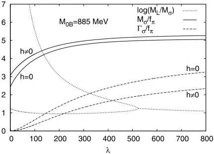
Fig. 1. Theλdependence of the real and imaginary parts of the
complex sigma pole p0 =Mσ−iΓσ/2 and of the Landau ghost
MLin the chiral limit and for the physical pion mass indicated with label h, 0 on the curves. ML is shown only in this latter case, for in the chiral limit there is very little difference.
propagator analytically continued between the two cuts to the second Riemann sheet in the form iG−1
σ(p0=κe−iφ,p=
0)=0. The pole is parametrized as p0=Mσ−iΓσ/2,with
the real and imaginary parts corresponding to the mass and the half-width of the sigma particle.
The solution for MσandΓσis shown in Fig. 1 both in
the chiral limit (h=mπ =0) and for the h,0 case.
Sim-ilar to the case of the O(N) model studied in Ref. [19], in the chiral limit the value of Mσ is a little smaller and the
value ofΓσlarger than in the h,0 case. Comparing Fig. 1
with Fig. 2 of Ref. [19] obtained in the O(N) model, that is without fermions, the Mσ(λ) curve moved slightly
up-ward, but theΓσ(λ) curve moved significantly downward,
which means that in the present case the phenomenologi-cally expected value [20] Mσ/Γσ ∼1 cannot be achieved
for any value of the couplingλ.Another difference is that
for low values ofλthere are two poles of Gσ on the
neg-ative imaginary axis in contrast to only one such pole in the O(N) model. These poles approach each other asλ
in-creases and after they collide at a given value ofλthere are
two complex poles at higherλ, one with positive and one
with negative real part. The imaginary part of the complex pole having positive real part is shown in Fig. 1 for the renormalization scale M0B = 885 MeV. As explained in the study done in the chiral limit in [8] for lower values of the renormalization scale the scale ML of the lower Lan-dau ghost on the imaginary axis comes even closer to Mσ
and as a result the spectral function of the sigma is heavily distorted. In order to avoid this and based on the ratio of
Mσ/Γσwe have chosenλ=400 and M0B=885 MeV. For these values Mσ = 456 MeV andΓσ = 221 MeV in the
chiral case, while Mσ =474 MeV andΓσ =152 MeV for
3 The
µ
q−
T
Phase diagram
The thermodynamics is determined by solving the field equations, i.e. (23) and the equations giving the depen-dence on T andµq of the two real mean fieldsΦand ¯Φ, which, when the full fermion propagator is replaced by the tree-level one have the form:
dU(Φ,Φ¯)
dΦ −2Nc
√
N
Z
k
k2 3Ek
d ˜f+ Φ(Ek)
dΦ +
d ˜f−
¯
Φ(Ek)
dΦ
+g2√NNc 2
˜
T0
F(mq)−TF(M)
d ˜Tβ(m
q)
dΦ +
d ˜Tβ,2 2 (mq)
dΦ
−M2 dS
β,1(M,m q)
dΦ +
dSβ,2(M,m q)
dΦ
!#
=0, (32)
where Ek = (k2 +m2q)
1
2 and M satisfies the gap equation
(27) or the relation M2 =h/v.The other equation is simi-lar to (32), the only difference is that the derivative is taken
with respect to ¯Φ.The integral in (32) is the contribution
of the fermionic trace-log integral, while the term propor-tional with g2 is the contribution of the quark-pion
two-loop integral in (9) given in Eq. (A35) of [7]. This term is disregarded for simplicity when solving the field equa-tions forΦand ¯Φ, and only in one case (see the last row
of Table 2) the complete equation (32) is solved in order to estimate the error made by neglecting it in all the other cases.
The tricritical point (TCP) and the critical end point (CEP) are identified as the points along the chiral phase transition line of theµq−Tphase diagram where a 1st order
phase transition turns with decreasingµq into a 2nd order or crossover transition, respectively. In case of a crossover, the temperature Tχof the chiral transition is defined as the
value where the derivative dv/dT has a minimum (inflec-tion point of v(T )), while the temperature Td of the de-confinement transition is obtained as the location of the maximum in dΦ/dT.The transition point in the case of
a 1st order phase transition is estimated by the inflection point located between the turning points of the multival-ued curvev(µq) obtained for a given constant temperature. Although the precise definition of the 1st order transition point is given by that value of the intensive parameter for which the two minima of the effective potential are
degen-erate, we adopt the definition based on the inflection point because we compute only the derivatives of the effective
potential with respect to the fields and propagators.
3.1 Phase transition in the chiral limit
In the chiral limit we solve the field equation (23) using the local approximation to the pion propagator (26) with
M2 =0 and neglect the term proportional withg2in (32). The critical temperature of the chiral transition Tχand the
pseudocritical temperature Td of the deconfinement tran-sition at vanishing chemical potential, and the location of the TCP are summarized in Table 1 for various forms of the
0 20 40 60 80 100 120 140 160 180
0 50 100 150 200 250 300 350
T [MeV]
µq [MeV] deconfinement chiral 2nd order 1st order spinodal TCP
Fig. 2. Phase diagrams obtained in the chiral limit without and with the inclusion of the Polyakov loop. The former has lower TTCPand for the latter we used Ulog(Φ,Φ¯) with T0 =208 MeV (upper curves) and with T0(µq) (middle curves). The deconfine-ment transition line is obtained from the inflection point ofΦ(T ).
Polyakov-loop potential. With the inclusion of the Polya-kov loop Tχ(µq =0) and TTCPincrease significantly com-pared with the values obtained earlier in [8] without the Polyakov loop, but it has little effect on the value ofµTCPq .
This increase in the value of Tχ(µq = 0) is basically de-termined by the value of the parameter T0of the Polyakov loop potential, while the value of TTCP shows no signifi-cant variation among different cases having the same value
of T0. One can also see, that as explained in [17], the use of the polynomial and logarithmic effective potentials for
the Polyakov loop, that is (10) and (12), drags the value of Tχ(µq =0) closer to the value of the parameter T0 than the use of UFuku(Φ,Φ¯) given in (14). In this latter case one obtains the smallest value for TTCP.
For T0 = 270 MeV the deconfinement transition line in theµq−T phase diagram is above the chiral transition line in all three variants of the effective potential for the
Polyakov loop. When the logarithmic effective potential
Ulog(Φ,Φ¯) is used either with a constant T0=208 MeV or with theµq-dependent T0 proposed in [2] one finds Td <
Tχatµq=0,but at a given value of the chemical potential the deconfinement transition line crosses the chiral
transi-U(Φ,Φ¯) T0 Tχ(0) Td(0) (T, µq)TCP
− − 139.0 − (60.7,277.0)
poly 270 185.6 229.0 (104.5,261.8) poly 208 168.2 176.5 (96.2,263.4) log 270 191.4 209.0 (109.4,261.2) log 208 167.6 162.4 (102.6,261.2) log T0(µq) 167.9 162.8 (84.3,266.9) Fuku − 176.5 193.0 (99.8,262.2) Table 1. The (pseudo)critical temperature (Td) Tχof the
tion line and remains above it for higher values ofµq.This
is shown in Fig. 2, where the deconfinement transition line is obtained from the inflection point ofΦ(T ).In contrast to
the case of constant T0,where basically the deconfinement transition line is not affected by the increase ofµq,with a
µq-dependent T0the deconfinement transition line strongly bends, staying close to the chiral line. The two lines cross just above the TCP.
In the case when T0(µq) is used, the lowering of the de-confinement transition results in the shrinking of the region of theµq−T plane for which Tχ < T <Td,already ob-served in Ref. [21]. Since the quantity measuring the quark content inside thermally excited particles carrying baryon number shows a pronounced change along the chiral phase transition line of this region, the region was identified in [17] with the so-called quarkyonic phase, a confining state made of quarks and is characterized by a high quark num-ber density and baryonic (three-quark state) thermal exci-tations.
Comparing our results on the phase diagram to those obtained in the chiral limit of the PNJL model one can no-tice differences of both qualitative and quantitative nature.
In the nonlocal PNJL model of Ref. [22] the deconfinement phase transition line starts atµq=0 below the chiral transi-tion line both for a polynomial and a logarithmic Polyakov-loop effective potential with T0=270 MeV, so that the two transition lines cross at finiteµq.In our case this happens only for the logarithmic potential with T0 = 208 MeV, as can be seen in Fig. 2. In [22,23] the values of Tχ(µq =0) and TTCPare much larger than in our case, while the value ofµTCPq is similar to ours.
3.2 Phase transition with a physical pion mass
In the approximation (28) for the pion propagator, which resum infinitely many orders in 1/√N,the phase
transi-tion at T = 0 turns with increasingµq from a crossover type into a first order transition at some value µcq > Mq, and in consequence there is a CEP in theµq−T phase dia-gram. The numerical results are summarized in Table 2 for
U(Φ,Φ¯) T0 Tχ(0) Td(0) Γχ (T, µq)CEP
− − 158.6 − 40.7 (13.5,328.6) poly 270 212.5 217.4 28.3 (32.9,328.8) poly 208 184.6 176.8 22.3 (30.6,328.8) log 270 209.7 209.3 12.0 (34.5,329.0) log 208 168.5 167.1 *43.0 (33.0,328.9) Fuku − 195.2 191.3 21.2 (31.8,328.8) poly 208 188.1 183.1 21.4 (32.2,329.0) Table 2. The temperatures Tχand Tdof the chiral and deconfine-ment transitions, the half-width at half maximumΓχof−dv/dT
atµq=0 (in the case marked with∗, due to the asymmetric shape of−dv/dT,the full width is given) and the location of the CEP in
units of MeV obtained using (28) for the pion propagator without and with the inclusion of the Polyakov loop. The contribution of the quark-pion setting-sun was kept in (32) only for the result of the last row.
0 20 40 60 80 100 120 140 160 180 200
0 50 100 150 200 250 300 350 400
T [MeV]
µq [MeV]
deconfinement chiral cross-over 1st order CEP
Fig. 3. Phase diagrams obtained for the physical value of the pion mass with the inclusion of the Polyakov loop. For the chiral tran-sition line which starts at higher T forµq=0 we used Upoly(Φ,Φ¯)
with T0=208 MeV and (28) for the pion propagator, for the other two phase diagrams we used the local approximation for the pion propagator and Ulog(Φ,Φ¯) with T0 =208 MeV (middle curves) and with T0(µq) (lower curves). The deconfinement transition line is obtained from the inflection point ofΦ(T ).
various forms of the Polyakov-loop potential reviewed in Sec. 2.2. Increasing the temperatureµcq decreases and the
first order chiral restoration becomes a crossover at a much lower temperature TCEPthan in the chiral case. The inclu-sion of the Polyakov loop increases significantly the value of TCEP,but, as in the chiral case, it has little effect on the value ofµCEPq .Neither the choice of the effective potential
for the Polyakov loop nor the value of T0has a significant effect on the value ofµCEPq .The result in the last row was
obtained by keeping in the field equation of the Polyakov loop (32) and its conjugate the contribution of the quark-pion setting-sun diagram, while in all other cases only the contribution of the fermionic trace-log was kept. Compar-ing the result in the last row of Table 2 with that of the second row obtained using the polynomial Polyakov-loop potential, one sees that the error we make by neglecting the setting-sun contribution in all other cases is fairly small.
The values of Tχ and Td at µq = 0 are mostly in-fluenced by the choice of the Polyakov effective
poten-tial and the value of T0 : they decrease with the decrease of T0 and by using the logarithmic potential instead of the polynomial one. Using the polynomial potential with
ap-proaches theµqaxis. This is even more the case here, with
a physical pion mass, since the deconfinement transition is a crossover and as such it happens in a relatively large temperature interval. However, the quarkyonic phase does not vanish completely as happens in [6], where quantum fluctuations are included using functional renormalization group methods.
4 Conclusions
Using the tree-level fermion propagator and some approx-imations for the self-consistent pion propagator obtained within a large-Nf expansion, we studied in the S U(2)L×
S U(2)Rchiral quark-meson model, in the chiral limit and for the physical value of the pion mass, the influence of the Polyakov loop on the chiral phase transition. When the local part of the approximate pion propagator resums in-finitely many orders in 1/Nf of fermionic contributions it is possible to find a CEP on the chiral phase transition line of the µq −T phase diagram. The inclusion of the Polyakov loop potential has a significant effect on TCEP and practically no effect onµCEPq obtained in the original
chiral quark-meson model, that is which does not contain the Polyakov loop. Using the logarithmic form Ulog(Φ,Φ¯) of the effective potential for the Polyakov loop with
pa-rameter T0 =208 MeV a crossing between the chiral and deconfinement transition lines was observed, with the lat-ter line starting atµq=0 slightly below the former one. In this case the existence of the quarkyonic phase is possible. It was shown in [7] that the result of resumming in the pion propagatorO(1/√N) fermionic fluctuations ob-tained with a strict expansion in 1/√N, while keeping the
fermion propagator unresummed, the phase transition soft-ens to the point that there is no CEP in theµq−T phase di-agram within a range 0< µq<500 MeV. For this reason it is an interesting question to what extent our results on the existence and location of the CEP would be modified by the use of the self-consistent propagator for fermions, and also by considering the more realistic S U(3)L×S U(3)R chiral quark-meson model.
Acknowledgments
This work is supported by the Hungarian Research Fund under Contracts No. T068108 and No. K77534.
References
1. W. Weise, Prog. Theor. Phys. Suppl. 174, 1 (2008). 2. B.-J. Schaefer, J. M. Pawlowski, and J. Wambach,
Phys. Rev. D 76, 074023 (2007).
3. B.-J. Schaefer, M. Wagner, and J. Wambach, Phys. Rev. D 81, 074013 (2010).
4. E. Nakano, B.-J. Schaefer, B. Stokic, B. Friman, K. Redlich, Phys. Lett. B682, 401 (2010).
5. V. Skokov, B. Friman, E. Nakano, K. Redlich, B.-J. Schaefer, Phys. Rev. D 82, 034029 (2010).
6. T. Herbst, J. Pawlowski, and B.-J. Schaefer, arXiv:1008.0081 [hep-ph].
7. G. Mark´o, Zs. Sz´ep, Phys. Rev. D 82, 065021 (2010). 8. A. Jakov´ac, A. Patk´os, Zs. Sz´ep, and P. Sz´epfalusy,
Phys. Lett. B582, 179 (2004).
9. C. P. Korthals Altes, R. D. Pisarski, and A. Sinkovics, Phys. Rev. D 61, 056007 (2000).
10. J. M. Luttinger and J.C. Ward, Phys. Rev. 118, 1417 (1960).
11. D. Dominici and U. Marini Bettolo Marconi, Phys. Lett. B319, 171 (1993).
12. G. Fej˝os, A. Patk´os, and Zs. Sz´ep, Phys. Rev. D 80, 025015 (2009).
13. R. D. Pisarski, Phys. Rev. D 62, 111501(R) (2000). 14. C. Ratti, M. A. Thaler, and W. Weise, Phys. Rev. D 73,
014019 (2006).
15. K. Fukushima, Phys. Lett. B591, 277 (2004).
16. C. Ratti, S. R¨oßner, M. A. Thaler, and W. Weise, Eur. Phys. J. C 49, 213 (2007).
17. K. Fukushima, Phys. Rev. D 77, 114028 (2008). 18. J. Zinn-Justin, Quantum Field Theory and Critical
Phenomena, 4th edition, (Oxford University Press, Oxford, 2002).
19. A. Patk´os, Zs. Sz´ep, and P. Sz´epfalusy, Phys. Lett. B537, 77 (2002).
20. I. Caprini, G. Colangelo, and H. Leutwyler, Phys. Rev. Lett. 96, 132001 (2006).
21. H. Abuki, R. Anglani, R. Gatto, G. Nardulli, and M. Ruggieri, Phys. Rev. D 78, 034034 (2008).
22. C. Sasaki, B. Friman, and K. Redlich, Phys. Rev. D 75, 074013 (2007).
23. P. Costa, C. A. de Sousa, M. C. Ruivo, and H. Hansen, Europhys. Lett. 86, 31001 (2009).