Condensed Unpredictability
Maciej Sk´orski1?, Alexander Golovnev2, and Krzysztof Pietrzak3??
1 University of Warsaw [email protected] 2 New York University [email protected]
3 IST Austria [email protected]
Abstract. We consider the task of deriving a key with high HILL en-tropy (i.e., being computationally indistinguishable from a key with high min-entropy) from an unpredictable source.
Previous to this work, the only known way to transform unpredictability into a key that wasindistinguishable from having min-entropy was via pseudorandomness, for example by Goldreich-Levin (GL) hardcore bits. This approach has the inherent limitation that from a source withkbits of unpredictability entropy one can derive a key of length (and thus HILL entropy) at mostk−2 log(1/) bits. In many settings, e.g. when dealing with biometric data, such a 2 log(1/) bit entropy loss in not an option. Our main technical contribution is a theorem that states that in the high entropy regime, unpredictability implies HILL entropy. Concretely, any variable K with |K| −d bits of unpredictability entropy has the same amount of so called metric entropy (against real-valued, determin-istic distinguishers), which is known to imply the same amount of HILL entropy. The loss in circuit size in this argument is exponential in the entropy gapd, and thus this result only applies for small d(i.e., where the size of distinguishers considered is exponential ind).
To overcome the above restriction, we investigate if it’s possible to first “condense” unpredictability entropy and make the entropy gap small. We show that any source withk bits of unpredictability can be condensed into a source of lengthkwithk−3 bits of unpredictability entropy. Our condenser simply “abuses” the GL construction and derives akbit key from a source with k bits of unpredicatibily. The original GL theorem implies nothing when extracting that many bits, but we show that in this regime, GL still behaves like a “condenser” for unpredictability. This result comes with two caveats (1) the loss in circuit size is exponential in
kand (2) we require that the source we start with hasnoHILL entropy (equivalently, one can efficiently check if a guess is correct). We leave it as an intriguing open problem to overcome these restrictions or to prove they’re inherent.
1
Introduction
Key-derivation considers the following fundamental problem: Given a joint dis-tribution (X, Z) whereX|Z (which is short for “X conditioned onZ”) is guar-anteed to have some kind of entropy, derive a “good” key K = h(X, S) from
X by means of some efficient key-derivation function h, possibly using public randomnessS.
In practice, one often uses a cryptographic hash function like SHA3 as the key derivation function h(.) [Kra10,DGH+04], and then simply assumes that h(.) behaves like a random oracle [BR93].
In this paper we continue the investigation of key-derivation with provable security guarantees, where we don’t make any computational assumption about h(.). This problem is fairly well understood for sources X|Z that have high min-entropy (we’ll formally define all the entropy notions used in 2 below), or are computationally indistinguishable from having so (in this case, we sayX|Z has high HILL entropy). In the case where X|Z hask bits of min-entropy, we can either use a strong extractor to derive a k−2 log−1 key that is-close to uniform, or a condenser to get a k bit key which is-close to a variable with k−log log−1 bits of min-entropy. Using extractors/condensers like this also works for HILL entropy, except that now we only get computational guarantees (pseudorandom/high HILL entropy) on the derived key.
Often one has to derive a key from a source X|Z which has no HILL en-tropy at all. The weakest assumption we can make onX|Z for any kind of key-derivation to be possible, is that X is hard to predict given Z. This has been formalized in [HLR07a] by saying that X|Z has k bits of unpredictability en-tropy, denotedHunp
s (X|Z)>k, if no circuit of sizescan predictX givenZ with advantage>2−k (to be more general, we allow an additional parameterδ
>0, and Hδ,sunp(X|Z) >k holds if (X, Z) is δ-close to some distribution (Y, Z) with Hunp
s (Y|Z)>k). We will also consider a more restricted notion, where we say that X|Z hask bits oflist-unpredictability entropy, denotedH∗unp
s (X|Z)>k, if it haskbits of unpredictability entropy relative to an oracleEqwhich can be used to verify the correct guess (Eqoutputs 1 on input X, and 0 otherwise).4 We’ll discuss this notion in more detail below. For now, let us just mention that for the important special case where it’s easy to verify if a guess for X is cor-rect (say, because we condition on Z = f(X) for some one-way function5 f), the oracle Eqdoes not help, and thus unpredictability and list-unpredictability coincide. The results proven in this paper imply that from a source X|Z with k bits of list-unpredictability entropy, it’s possible to extract a k bit key with k−3 bits of HILL entropy
Proposition 1. Consider a joint distribution (X, Z) over {0,1}n × {0,1}m where
Hs,γ∗unp(X|Z)>k (1)
4 We chose this name as having access to
Eqis equivalent to being allowed to output a list of guesses. This is very similar to the well known concept of list-decoding.
5 To be precise, this only holds for injective one-way functions. One can generalise
list-unpredictability and letEq output 1 on some setX, and the adversary wins if she outputs anyX ∈ X. Our results (in particular Theorem1) also hold for this more general notion, which captures general one-way functions by lettingX =f−1(f(X))
Let S ∈ {0,1}n×k be uniformly random and K = XTS ∈ {0,1}k, then the unpredictability entropy ofK is
Hs/2unp2kpoly(m,n),γ(K|Z, S)>k−3 (2)
and the HILL entropy ofK is
Ht,+γHILL(K|Z, S)>k−3 (3)
with6 t=s· 7 22kpoly(m,n).
Proposition 1follows from two results we prove in this paper.
First, in Section4we prove Theorem1which shows how to “abuse” Goldreich-Levin hardcore bits by generating akbit keyK=XTS from a sourceX|Z with kbits of list-unpredictability. The Goldreich-Levin theorem [GL89] implies noth-ing about the pseudorandomness of K|(Z, S) when extracting that many bits. Instead, we prove that GL is a good “condenser” for unpredictability entropy: if X|Z has kbits of list-unpredictability entropy, thenK|(Z, S) hask−3 bits of unpredictability entropy (note that we start with list-unpredictability, but only end up with “normal” unpredictability entropy). This result is used in the first step in Proposition1, showing that (1) implies (2).
Second, in Section5we prove our main result, Theorem2which states that any sourceX|Zwhich has|X| −dbits of unpredictability entropy, has the same amount of HILL entropy (technically, we show that it implies the same amount of metric entropy against deterministic real-valued distinguishers. This notion implies the same amount of HILL entropy as shown by Barak et al. [BSW03]). The security loss in this argument is exponential in the entropy gapd. Thus, if dis very large, this argument is useless, but if we first condense unpredictability as just explained, we have a gap of onlyd= 3. This result is used in the second step in Proposition 1, showing that (2) implies (3). In the two sections below we discuss two shortcomings of Theorem1 which we hope can be overcome in future work.7
On the dependency on 2k in Theorem 1. As outlined above, our first result is Theorem1, which shows how to condense a source withk bits of list-unpredictability into a k bit key having k−3 bits of unpredictability entropy. The loss in circuit size is 22kpoly(m, n), and it’s not clear if the dependency on 2k
6 We denote withpoly(m, n) some fixed polynomial in (n, m), but it can denote
dif-ferent polynomial throughout the paper. In particular, thepolyhere is not the same as in (2) as it hides several extra terms.
7 After announcing this result at a workshop, we learned that Colin Jia Zheng proved
a weaker version of this result. Theorem 4.18 in this PhD thesis, which is available viahttp://dash.harvard.edu/handle/1/11745716also states thatkbits of unpre-dictability imply k bits of HILL entropy. Like in our case, the loss in circuit size in his proof is polynomial in −1, but it’s also exponential inn (the length ofX),
is necessary here, or if one can replace the dependency on 2k with a dependency onpoly(−1) at the price of an extra term in the distinguishing advantage. In many settings log(−1) is in the order of k, in which case the above difference is not too important. This is for example the case when considering ak bit key for a symmetric primitive like a block-cipher, where one typically assumes the hardness of the cipher to be exponential in the key-length (and thus, if we want to be in the same order, we have log(−1) =Θ(k)). In other settings,kcan be superlinear in log(−1), e.g., if the the high entropy string is used to generate an RSA key.
List vs. normal Unpredictability. Our Theorem1shows how to condense a source where X|Z haskbits of list-unpredictability entropy into ak bit string withk−3 bits unpredictability entropy. It’s an open question to which extent it’s necessary to assumelist-unpredictability here, maybe “normal” unpredictability is already sufficient? Note that list-unpredictability is a lower bound for unpre-dictability as one always can ignore theEqoracle, i.e.,Hunp
,s(X|Z)>H,s∗unp(X|Z), and in general, list-unpredictability can be much smaller than unpredictability entropy.8
Interestingly, we can derive ak bit key with almostk bits of HILL entropy from a sourceX|Z whichkbits unpredictability entropyH,sunp(X|Z)>kin two extreme cases, namely, if either
1. ifX|Z has basically no HILL entropy (even against small circuits). 2. or when X|Z has (almost)k bits of (high quality) HILL entropy. In case 1. we observe that if HHILL
,t (X|Z)≈0 for some t s, or equivalently, given Z we can efficiently distinguishX from any X0 6=X, then theEq oracle used in the definition of list-unpredictability can be efficiently emulated, which means it’s redundant, and thusX|Zhas the same amount of list-unpredictability and unpredictability entropy, Hunp
s,(X|Z) ≈ H ∗unp
s0,0(X|Z) for (0, s0) ≈ (, s).
Thus, we can use Theorem 1 to derive a k bit key with k−O(1) bits of HILL entropy in this case. In case 2., we can simply use any condenser for min-entropy to get a key with HILL entropy k−log log−1 (cf. Figure 2). As condensing almost all the unpredictability entropy into HILL entropy is possible in the two extreme cases where X|Z has either no or a lot of HILL entropy, it seems con-ceivable that it’s also possible in all the in-between cases (i.e., without making any additional assumptions aboutX|Z at all).
GL vs. Condensing. Let us stress as this point that, because of the two issues discussed above, our result does not always allow generate more bits with high HILL entropy than just using the Goldreich-Levin theorem. Assumingk bits of unpredictability we getk−3 of HILL, whereas GL will only givek−2 log(1/). But as currently our reduction has a quantitatively larger loss in circuit size
8 E.g., letX by uniform over{0,1}nandZ arbitrary, but independent ofX, then for
s = exp(n) we haveHunp
s (X|Z) =n butHs∗unp(X|Z) = 0 as we can simply invoke
than the GL theorem, in order to get HILL entropy of the same quality (i.e., secure against (s, δ) adversaries for some fixed (s, δ)) we must consider the un-predictability entropy of the sourceX|Zagainst more powerful adversaries than if we’re about to use GL. And in general, the amount of unpredictability (or any other computational) entropy ofX|Zcan decrease as we consider more powerful adversaries.
2
Entropy Notions
In this section we formally define the different entropy notions considered in this paper. We denote with Dsrand,{0,1} the set of all probabilistic circuits of size s with boolean output, andDrand,[0,1]s denotes the set of all probabilistic circuits withreal-valued output in the range [0,1]. The analogous deterministiccircuits are denotedDsdet,{0,1} andDdet,[0,1]s . We useX ∼,sY to denote computational indistinguishability of variablesX andY, formally9
X ∼,sY ⇐⇒ ∀C∈ Dsrand,{0,1} : |Pr[C(X) = 1]−Pr[C(Y) = 1]|6 (4) X ∼ Y denotes thatX and Y have statistical distance, i.e.,X ∼,∞Y, and withX ∼Y we denote that they’re identically distributed. WithUn we denote the uniform distribution over{0,1}n.
Definition 1. The min-entropyof a random variableX with supportX is
H∞(X) =−log2max
x∈XPr[X =x]
For a pair (X, Z) of random variables, theaverage min-entropy ofX condi-tioned onZ is
e
H∞(X|Z) = −log2 E
z←Zmaxx Pr[X =x|Z =z] = −log2z←EZ2
−H∞(X|Z=z)
HILL entropy is a computational variant of min-entropy, whereX (conditioned onZ) haskbits of HILL entropy, if it cannot be distinguished from someY that (conditioned onZ) haskbits of min-entropy, formally
Definition 2 ( [HILL99], [HLR07a]). A random variableX has HILL en-tropy k, denoted by Hε,sHILL(X) ≥ k, if there exists a distribution Y satisfying H∞(Y)≥kandX ∼ε,sY.
Let (X, Z) be a joint distribution of random variables. Then X has condi-tional HILL entropykconditioned onZ, denoted byHHILL
ε,s (X|Z)≥k, if there exists a joint distribution(Y, Z)such thatHe∞(Y|Z)≥kand(X, Z)∼ε,s(Y, Z).
9 Let us mention that the choice of the distinguisher class in (4) irrelevant (up to a
small additive difference in circuit size), we can replaceDsrand,{0,1} with any of the
Barak, Sahaltiel and Wigderson [BSW03] define the notion of metric entropy, which is defined like HILL, but the quantifiers are exchanged. That is, instead of asking for a single distribution (Y, Z) that fools all distinguishers, we only ask that for every distinguisherD, there exists such a distribution. For reasons discussed in Section2, in the definition below we make the class of distinguishers considered explicit.
Definition 3 ( [BSW03], [FR12]). Let(X, Z)be a joint distribution of ran-dom variables. Then X has conditional metric entropy kconditioned on Z (against probabilistic boolean distinguishers), denoted byHε,sMetric,rand,{0,1}(X|Z)≥ k, if for every D∈ Drand,s {0,1} there exists a joint distribution (Y, Z) such that
e
H∞(Y|Z)≥k and
|Pr[D(X, Z) = 1]−Pr[D(Y, Z) = 1]|6
More generally, for class∈ {rand, det}, range∈ {[0,1],{0,1}}, HMetric,class,range
ε,s (X|Z)≥kif for everyD∈ Dclass,ranges such a(Y, Z)exists. Like HILL entropy, also unpredictability entropy, which we’ll define next, can be seen as a computational variant of min-entropy. Here we don’t require indistin-guishability as for HILL entropy, but only that the variable is hard to predict.
Definition 4 ( [HLR07a]). X hasunpredictability entropy kconditioned onZ, denoted byHunp
,s(X|Z)≥k, if(X, Z)is(, s)indistinguishable from some (Y, Z), where no probabilistic circuit of size scan predictY givenZ with proba-bility better than 2−k, i.e.,
Hs,unp(X|Z)≥k ⇐⇒ ∃(Y, Z),(X, Z)∼ε,s(Y, Z)∀C,|C|6s : Pr
(y,z)←(Y,Z)[C(z) =y]62 −k (5) We also define a notion called “list-unpredictability”, denotedH∗unp
,s (X|Z)≥k, which holds if Hunp
,s(X|Z) ≥ k as in (5), but where C additionally gets oracle access to a functionEq(.)which outputs1 on inputyand0otherwise. So,Ccan efficiently test if some candidate guess fory is correct.10
Remark 1 (The parameter). The parameter in the definition above is not really necessary, following [HLR07b], we added it so we can have a “smooth” notion, which is easier to compare to HILL or smooth min-entropy. If = 0, we’ll simply omit it, then the definition simplifies to
Hsunp(X|Z)≥k ⇐⇒ Pr
(x,z)←(X,Z)[C(z) =x]62 −k
Let us also mention that unpredictability entropy is only interesting if the con-ditional part Z is not empty as (already forsthat is linear in the length ofX)
10We name this notion ”list-unpredictability” as we get the same notion when instead
of giving Coracle access to Eq(.), we allow C(z) to output a list of guesses for y, not just one value, and require that Pr(y,z)←(Y,Z)[y∈ C(z)] 6 2−k. This notion is
we haveHunp
s (X) =H∞(X) which can be seen by considering the circuitC(that gets no input as Z is empty) which simply outputs the constantxmaximizing Pr[X =x].
Metric vs. HILL. We will use a lemma which states that deterministic real-valued metric entropy implies the same amount of HILL entropy (albeit, with some loss in quality). This lemma has been proven by [BSW03] for the uncon-ditional case, i.e., when Z in the lemma below is empty, it has been observed by [FR12,CKLR11] that the proof also holds in the conditional case as stated below
Lemma 1 ( [BSW03,FR12,CKLR11]).For any joint distribution (X, Z)∈ {0,1}n× {0,1}mand any , δ, k, s
H,sMetric,det,[0,1](X|Z)>k ⇒ H
HILL
+δ,s·δ2/(m+n)(X|Z)>k
Note that in Definition 2 of HILL entropy, we only consider security against probabilistic boolean distinguishers (as ∼,s was defined this way), whereas in Definiton 3 of metric entropy we make the class of distinguishers explicit. The reason for this is that in the definition of HILL entropy the class of distinguishers considered is irrelevant (except for a small additive degradation in circuit size, cf. [FR12, Lemma 2.1]).11 Unlike for HILL, for metric entropy the choice of the distinguisher class does matter. In particular, deterministic boolean metric entropy H,sMetric,det,{0,1}(X|Y) > k is only known to imply deterministic real-valued metric entropy H+δ,sMetric,det,[0,1](X|Y)>k−log(δ−1), i.e., we must allow for a δ > 0 loss in distinguishing advantage, and this will at the same time result in a loss of log(δ−1) in the amount of entropy. For this reason, it is crucial that in Theorem2 we show that unpredictability entropy implies deterministic real-valued metric entropy, so we can then apply Lemma 1 to get the same amount of HILL entropy. Dealing with real-valued distinguishers is the main source of technical difficulty in the proof of the Theorem2, proving the analogous statement for deterministicboolean distinguishers is much simpler.
3
Known Results on Provably Secure Key-Derivation
We say that a cryptographic scheme has securityα, if no adversary (from some class of adversaries like all polynomial size circuits) can win some security game with advantage > α if the scheme is instantiated with a uniformly random string.12Below we will distinguish between unpredictability applications, where
11This easily follows from the fact that in the definition (4) of computational
indistin-guishability the choice of the distinguisher class is irrelevant.
12We’ll call this string “key”. Though in many settings (in particular when keys are
the advantage bounds the probability of winning some security game (a typical example are digital signature schemes, where the game captures the existential unforgeability under chosen message attacks), and indistinguishability applica-tions, where the advantage bounds the distinguishing advantage from some ideal object (a typical example is the security definition of pseudorandom generators or functions).
3.1 Key-Derivation from Min-Entropy
Strong Extractors. Let (X, Z) be a source whereHe∞(X|Z)>k, or equivalently, no adversary can guessX givenZ with probability better than 2−k (cf. Def.1). Consider the case where we want to derive a keyK=h(X, S) that is statistically close to uniform given (Z, S). For example, X could be some physical source (like statistics from keystrokes) from which we want to generate almost uniform randomness. HereZ models potential side-information the adversary might have onX. This setting is very well understood, and such a key can be derived using a strong extractor as defined below.
Definition 5 ( [NZ93], [DORS08]). A function Ext : {0,1}n × {0,1}d → {0,1}` is an average-case (k, )-strong extractor if for every distribution (X, Z) over{0,1}n×{0,1}mwith
e
H∞(X|Z)>kandS∼Ud, the distribution(Ext(X, S), S, Z) has statistical distance to(Um, S, Z).
ExtractorsExtas above exist with `=k−2 log(1/) [HILL99]. Thus, from any (X, Z) where He∞(X|Z) > k we can extract a key K = Ext(X, S) of length k−2 log(1/) that isclose to uniform [HILL99]. The entropy gap 2 log(1/) is optimal by the so called “RT-bound” [RTS00], even if we assume the source is efficiently samplable [DPW14].
If instead of using a uniform`bit key for an αsecure scheme, we use a key that is close to uniform, the scheme will still be at least β =α+ secure. In order to get security β that is of the same order as α, we thus must set≈α. When the available amountkof min-entropy is small, for example when dealing with biometric data [DORS08,BDK+05], a loss of 2 log(1/) bits (that’s 160 bits for a typical security level= 2−80) is often unacceptable.
Condensers. The above bound is basically tight for many indistinguishability applications like pseudorandom generators or pseudorandom functions.13 For-tunately, for many applications a close to uniform key is not necessary, and a key |K| with min-entropy |K| −∆ for some small ∆ is basically as good as a uniform one. This is the case for allunpredictability applications, which includes
13For example, consider a pseudorandom functionF:{0,1}k× {0,1}a→ {0,1}and a
keyK that is uniform over all keys whereF(K,0) = 0, this distribution is ≈1/2 close to uniform and has min-entropy≈ |K| −1, but the security breaks completely as one can distinguishF(Uk, .) fromF(K, .) with advantageβ≈1/2 (by quering on
OWFs, digital-signatures and MACs.14 It’s not hard to show that if the scheme is αsecure with a uniform key it remains at least β =α2∆ secure (against the same class of attackers) if instantiated with any keyK that has|K| −∆bits of min-entropy.15 Thus, for unpredictability applications we don’t have to extract an almost uniform key, but “condensing” X into a key with |K| −∆ bits of min-entropy for some small∆is enough.
[DPW14] show that a (log+ 1)-wise independent hash function Cond : {0,1}n× {0,1}d→ {0,1}`is a condenser with the following parameters. For any (X, Z) whereHe∞(X|Z)>`, for a random seedS (used to sample a (log+ 1)-wise independent hash function), the distribution (Cond(X, S), S) is close to a distribution (Y, S) where He∞(Y|Z) > `−log log(1/). Using such an ` bit key (condensed from a source with ` bits min-entropy) for an unpredictability application that is αsecure (when using a uniform ` bit key), we get security β 6 α2log log(1/)+, which setting =α gives β 6α(1 + log(1/α)) security, thus, security degrades only by a logarithmic factor.
3.2 Key-Derivation from Computational Entropy
The bounds discussed in this section are summarised in Figures 1 and 2 in AppendixA. The last row of Figure2is the new result proven in this paper.
HILL Entropy. As already discussed in the introduction, often we want to derive a key from a distribution (X, Z) where there’s no “real” min-entropy at all
e
H∞(X|Z) = 0. This is for example the case whenZis the transcript (that can be observed by an adversary) of a key-exchange protocol like Diffie-Hellman, where the agreed valueX =gab is determined by the transcriptZ = (ga, gb) [Kra10, GKR04]. Another setting where this can be the case is in the context of side-channel attacks, where the leakage Z from a device can completely determine its internal stateX.
IfX|Z haskbits of HILL entropy, i.e., is computationally indistinguishable from having min-entropy k(cf. Def. 2) we can derive keys exactly as described above assumingX|Z hadkbits of min-entropy. In particular, if X|Z has|K|+ 2 log(1/) bits of HILL entropy for some negligible, we can derive a keyKthat is pseudorandom, and ifX|Zhas|K|+ log log(1/) bits of HILL entropy, we can
14 [DY13] identify an interesting class of applications called “square-friendly”, this class
contains all unpredictability applications, and some indistinguishability applications like weak PRFs (which are PRFs that can only be queried on random inputs). This class of applications remains somewhat secure even for a small entropy gap∆: For
∆= 1 the security isβ≈√α. This is worse that theβ= 2αfor unpredictability applications, but much better than the complete loss of securityβ ≈1/2 required for some indistinguishability apps like (standard) PRFs.
15Assume some adversary breaks the scheme, say, forges a signature, with advantageβ
derive a key that is almost as good as a uniform one for any unpredictability application.
Unpredictability Entropy. Clearly, the minimal assumption we must make on a distribution (X, Z)∈ {0,1}n×{0,1}mfor any key derivation to be possible at all is thatXis hard to compute givenZ, that is,X|Zmust have some unpredictabil-ity entropy as in Definition4. Goldreich and Levin [GL89] show how to generate pseudorandom bits from such a source. In particular, the Goldreich-Levin theo-rem implies that ifX|Z has at least 2 log−1 bits of list-unpredictability, then the inner productRTX ofX with a random vectorRisindistinguishable from uniformly random (the loss in circuit size ispoly(n, m)/4). Using the chain rule for unpredictability entropy,16 we can generate an ` = k−2 log−1 bit long pseudorandom string that is`indistinguishable (the extra`factor comes from taking the union bound over all bits) from uniform.
Thus, we can turnkbits of list-unpredictability intok−2 log−1bits of pseu-dorandom bits (and thus also that much HILL entropy) with quality roughly . The question whether it’s possible to generate significantly more than k− 2 log−1 of HILL entropy from a source with k bits of (list-)unpredictability seems to have never been addressed in the literature before. The reason might be that one usually is interested in generating pseudorandom bits (not just HILL entropy), and for this, the 2 log−1entropy loss is inherent. The observation that for many applications high HILL entropy is basically as good as pseudorandom-ness is more recent, and recently gained attention by its usefulpseudorandom-ness in the context of leakage-resilient cryptography [DP08,DY13].
In this paper we prove that it’s in fact possible to turn almost all list-unpredictability into HILL entropy.
4
Condensing Unpredictability
Below we state Theorem1 whose proof is in Appendix B, but first, let us give some intuition. LetX|Z havekbits of list-unpredictability, and assume we start extracting Goldreich-Levin hardcore bits A1, A2, . . . by taking inner products Ai=RTiX for randomRi. The first extracted bitsA1, A2, . . .will be pseudoran-dom (given theRiandZ), but with every extracted bit, the list-unpredictability can also decrease by one bit. As the GL theorem requires at least 2 log−1 bits of list-unpredictability to extract an secure pseudorandom bit, we must stop afterk−2 log−1bits. In particular, the more we extract, the worse the pseudo-randomness of the extracted string becomes. Unlike the original GL theorem, in our Theorem1we only argue about the unpredictability of the extracted string, and unpredictability entropy has the nice property that it can never decrease, i.e., predictingA1, . . . , Ai+1 is always at least as hard as predictingA1, . . . , Ai.
16Which states that if X|Z has k bits of list-unpredictability, then for any
Thus, despite the fact that oncei approacheskit becomes easier and easier to predictAi (givenA1, . . . , Ai−1, Z and theRi’s)17 this hardness will still add up tok−O(1) bits of unpredictability entropy.
The proof is by contradiction, we assume thatA1, . . . , Ak can be predicted with advantage 2−k+3 (i.e., does not have k−3 bits of unpredictability), and then use such a predictor to predictX with advantage>2−k, contradicting the kbit list-unpredictability ofX|Z.
IfA1, . . . , Ak can be predicted as above, then there must be an indexj s.t. Aj can be predicted with good probability conditioned on A1, . . . , Aj−1 being correctly predicted. We then can use the Goldreich-Levin theorem, which tells us how to findX given such a predictor. Unfortunately,jcan be close tok, and to apply the GL theorem, we first need to find the right values forA1, . . . , Aj−1on which we condition, and also can only use the predictor’s guess for Aj if it was correct on the firstj−1 bits. We have no better strategy for this than trying all possible values, and this is the reason why the loss in circuit size in Theorem1 depends on 2k.
In our proof, instead of using the Goldreich-Levin theorem, we will actually use a more fine-grained variant due to Hast which allows to distinguish between errors and erasures (i.e., cases where we know that we don’t have any good guess. As outlined above, this will be the case whenever the predictor’s guess for the firstj−1 inner products was wrong, and thus we can’t assume anything about the jth guess being correct). This will give a much better quantitative bound than what seems possible using GL.
Theorem 1 (Condensing Upredictability Entropy). Consider any distri-bution (X, Z) over{0,1}n× {0,1}m where
H,s∗unp(X|Z)>k
then for a random R← {0,1}k×n
H,tunp(R.X|Z, R)>k−∆ where18
t= s
22kpoly(m, n) , ∆= 3
5
High Unpredictability implies Metric Entropy
In this section we state our main results, showing thatkbits of unpredictability entropy imply the same amount of HILL entropy, with a loss exponential in the “entropy gap”. The proof is in AppendixC.
17The only thing we know about the last extracted bitA
kis that it cannot be predicted
with advantage > 0.75, more generally, Ak−j cannot be predicted with advantage
1/2 + 1/2j+2.
18We can set∆to be any constant>1 here, but choosing a smaller∆would imply a
Theorem 2 (Unpredictability Entropy Implies HILL Entropy).For any distribution(X, Z)over{0,1}n× {0,1}m, ifX|Z has unpredictability entropy
Hγ,sunp(X|Z)>k (6) then, with∆=n−kdenoting the entropy gap,X|Z has (real valued, determin-istic) metric entropy
H+γ,tMetric,det,[0,1](X|Z)>k for t=Ω
s·
5 25∆log2(2∆−1)
(7)
By Lemma1this further implies that X|Z has, for any δ >0, HILL entropy
H+δ+γ,Ω(tδHILL 2/(n+m))(X|Z)>k which for=δ=γ is
H3,Ω(sHILL ·7/25∆(n+m) log2(2∆−1))(X|Z)>k
References
BDK+05. Xavier Boyen, Yevgeniy Dodis, Jonathan Katz, Rafail Ostrovsky, and Adam
Smith. Secure remote authentication using biometric data. In Ronald Cramer, editor,EUROCRYPT 2005, volume 3494 ofLNCS, pages 147–163. Springer, May 2005.
BR93. Mihir Bellare and Phillip Rogaway. Random oracles are practical: A paradigm for designing efficient protocols. In V. Ashby, editor,ACM CCS 93, pages 62–73. ACM Press, November 1993.
BSW03. B. Barak, R. Shaltiel, and A. Wigderson. Computational Analogues of Entropy. In S. Arora, K. Jansen, J. D. P. Rolim, and A. Sahai, editors,
RANDOM-APPROX 03, volume 2764 of LNCS, pages 200–215. Springer,
2003.
CKLR11. Kai-Min Chung, Yael Tauman Kalai, Feng-Hao Liu, and Ran Raz. Memory delegation. In Phillip Rogaway, editor, CRYPTO 2011, volume 6841 of LNCS, pages 151–168. Springer, August 2011.
DGH+04. Yevgeniy Dodis, Rosario Gennaro, Johan H˚astad, Hugo Krawczyk, and Tal
Rabin. Randomness extraction and key derivation using the CBC, cascade and HMAC modes. In Matthew Franklin, editor, CRYPTO 2004, volume 3152 ofLNCS, pages 494–510. Springer, August 2004.
DORS08. Y. Dodis, R. Ostrovsky, L. Reyzin, and A. Smith. Fuzzy Extractors: How to Generate Strong Keys from Biometrics and Other Noisy Data. SIAM Journal on Computing, 38(1):97–139, 2008.
DP08. Stefan Dziembowski and Krzysztof Pietrzak. Leakage-resilient cryptogra-phy. In49th FOCS, pages 293–302. IEEE Computer Society Press, October 2008.
DPW14. Yevgeniy Dodis, Krzysztof Pietrzak, and Daniel Wichs. Key derivation without entropy waste. InEUROCRYPT 14, LNCS. Springer, 2014. DY13. Yevgeniy Dodis and Yu Yu. Overcoming weak expectations. In Amit Sahai,
FR12. Benjamin Fuller and Leonid Reyzin. Computational entropy and informa-tion leakage. Cryptology ePrint Archive, Report 2012/466, 2012. http: //eprint.iacr.org/.
GKR04. Rosario Gennaro, Hugo Krawczyk, and Tal Rabin. Secure Hashed Diffie-Hellman over non-DDH groups. In Christian Cachin and Jan Camenisch, ed-itors,EUROCRYPT 2004, volume 3027 ofLNCS, pages 361–381. Springer, May 2004.
GL89. Oded Goldreich and Leonid A. Levin. A hard-core predicate for all one-way functions. In21st ACM STOC, pages 25–32. ACM Press, May 1989. Has03. Gustav Hast. Nearly one-sided tests and the Goldreich-Levin predicate.
In Eli Biham, editor, EUROCRYPT 2003, volume 2656 of LNCS, pages 195–210. Springer, May 2003.
HILL99. Johan H˚astad, Russell Impagliazzo, Leonid A. Levin, and Michael Luby. A pseudorandom generator from any one-way function. SIAM Journal on Computing, 28(4):1364–1396, 1999.
HLR07a. C.-Y. Hsiao, C.-J. Lu, and L. Reyzin. Conditional Computational Entropy, or Toward Separating Pseudoentropy from Compressibility. In M. Naor, editor,EUROCRYPT 07, volume 4515 ofLNCS, pages 169–186. Springer, 2007.
HLR07b. Chun-Yuan Hsiao, Chi-Jen Lu, and Leonid Reyzin. Conditional compu-tational entropy, or toward separating pseudoentropy from compressibility. In Moni Naor, editor, EUROCRYPT 2007, volume 4515 ofLNCS, pages 169–186. Springer, May 2007.
Kra10. Hugo Krawczyk. Cryptographic extraction and key derivation: The HKDF scheme. In Tal Rabin, editor,CRYPTO 2010, volume 6223 ofLNCS, pages 631–648. Springer, August 2010.
NZ93. Noam Nisan and David Zuckerman. More deterministic simulation in logspace. In25th ACM STOC, pages 235–244. ACM Press, May 1993. RTS00. Jaikumar Radhakrishnan and Amnon Ta-Shma. Bounds for dispersers,
A
Figures
Deriving a (pseudo)random key of length|K|=k−2 log−1
from a source (X, Z)∈ {0,1}n× {0,1}mwhereX|Zhaskbits (min/HILL/list-unpredictability) entropy
Entropy Entropy quantity and Derive keyKof Quality of derived key
type quality of source lengthk−2 log−1as HHILL
0,s0(K|Z, S) =k−2 log−1=|K|
equivalently (K, Z, S)∼0,s0(U|K|, Z, S)
min He∞(X|Z) =k K=Ext(X, S) 0= s0=∞
HILL HHILL
δ,s (X|Z) =k K=Ext(X, S) 0=+δ s0≈s
Unpredict. H∗unp
δ,s (X|Z) =k K=GL(X, S) =S
TX 0=m+δ s0=s·4/poly(m, n)
Fig. 1. Bounds on deriving a (pseudo)random keyKof length|K|=k−2 log−1 bit from a sourceX|Z withkbits of min, HILL or list-unpredictability entropy. Extis a strong extractor (e.g. leftover hashing), andGLdenotes the Goldreich-Levin construc-tion, which forX∈ {0,1}nandS∈ {0,1}n×|K|is simply defined asGL(X, S) =STX.
Leftover hashing requires a seed of length |S|= 2n(extractors with a much shorter seed|S|=O(logn+ log−1) that extractk−2 log−1−O(1) bits also exist), whereas
Goldreich-Levin requires a longer |S| = |K|n bit seed. The above bound for HILL entropy even holds if X|Z only hask bits of probabilistic boolean metric entropy (a notion implying the same amount of HILL entropy, albeit with a loss in circuit size), as shown in Theorem 2.5 of [FR12]
Derivingkbit keyKwith high HILL entropy fromX|Zwithkbits (min/HILL/list-unpredictability) entropy Entropy Entropy quantity and Derive key of Quantity and quality of HILL entropy ofK
type quality of soucre length|K|=kas HHILL
0,s0(K|Z, S)>k−∆
min He∞(X|Z) =k K=Cond(X, S) 0= s0=∞ ∆= log log−1
HILL HHILL
δ,s (X|Z) =k K=Cond(X, S) 0=+δ s0≈s ∆= log log−1
Unpredict. H∗unp
δ,s (X|Z) =k K=GL(X, S) =S
TX 0=+δ s0=s·7/22kpoly(m, n) ∆= 3
Fig. 2. Bounds on deriving a key of lengthkwith min (or HILL) entropyk−∆from a source X|Z withk bits of min, HILL or unpredictability entropy. Cond denotes a (log+ 1) wise independent hash function, which is shown to be a good condenser (as stated in the table) for min-entropy in [DPW14]. The bounds for HILL entropy follow directly from the bound for min-entropy. The last row follows from the results in this paper as stated in Proposition1.
B
Proof of Theorem
1
Theorem 3 ( [Has03]). There is an algorithm LDthat, on input l andnand with oracle access to a binary Hadamard code of x (where |x|=n) with an e-fraction of errors and an s-fraction of erasures, can output a list of2l elements in time O(nl2l) asking n2l oracle queries such that the probability that x is contained in the list is at least 0.8 if l > log2(20n(e+c)/(c−e)2+ 1), where c= 1−s−e(the fraction of the correct answers from the oracle).
We’ll often consider sequencesv1, v2, . . . of values and will use the notation vb
a to denote (va, . . . , vb), withvab=∅ ifa > b.vb is short for vb1= (v1, . . . , vb). Proof (of Theorem 1).It’s sufficient to prove the theorem for= 0, the general case>0 then follows directly by the definition of unpredictability entropy. To prove the theorem we’ll prove its contraposition
Htunp(R.X|Z, R)< k−∆ ⇒ Hs∗unp(X|Z)< k (8) The left-hand side of (8) means there exists a circuitAof size|A|6tsuch that
Pr
(x,z)←(X,Z),r←{0,1}k×n[A(z, r) =r.x]>2
−k+∆ (9)
It will be convenient to assume thatAinitially flips a coinb, and ifb= 0 outputs a uniformly random guess. This loses at most a factor 2 inA’s advantage, i.e.,
Pr
(x,z)←(X,Z),r←{0,1}k×n[A(z, r) =r.x]>2
−k+∆−1 (10)
but now we can assume that for anyz, r andw∈ {0,1}k
Pr[A(z, r) =w]>2−k−1 (11) Using Markov eq.(10) gives us
Pr
(x,z)←(X,Z)[r←{0,1Pr}k×n[A(z, r) =r.x]>2
−k+∆−2]
>2−k+∆−2 (12)
We call (x, z)∈supp[(X, Z)] “good” if
(x, z) is good ⇐⇒ Pr
r←{0,1}k×n[A(z, r) =r.x]>2
−k+∆−2 (13)
Note that by eq.(12), (z, x)←(Z, X) is good with probability>2−k+∆−2. We will useAto construct a new circuitBof sizes=O(t22kpoly(n)) where
Pr (x,z)←(X,Z)
[B(z) =x|(x, z) is good]>1/2 (14)
Which with (14) and (12) further gives
Pr (x,z)←(X,Z)
[B(z) =x] = Pr[B(z) =x|(x, z) is good]·Pr[(x, z) is good]
contradicting the right-hand side of (8), and thus proving the theorem.
We’ll now constructBsatisfying (14), for this, consider any good (x, z). Let R =Rk = (R
1, . . . , Rk) be uniformly random and let A =Ak = (A1, . . . , Ak) whereAi=Ri.x.
Let ˆA←A(z, R) and definei = PrR[ ˆAi =Ai|Aˆi−1 =Ai−1]. Using (13) in the last step
k
Y
i=1 i= Pr
R[A= ˆA] = PrR[A(z, R) =R.x]>2
−k+∆−2
Thus, here exists anis.t.,i>2
−k+∆−2
k = 1
2+δwithδ≈ ∆−2
k · ln(2)
2 . We fix this i(we don’t know whichiis good, and later will simply try all of them). Then
ERi−1[ Pr Ri,Rki+1
[ ˆAi=Ai |Aˆi−1=Ai−1]]>1/2 +δ
Using Markov
Pr Ri−1[RPr
i,Rki+1
[ ˆAi=Ai |Aˆi−1=Ai−1]>1/2 +δ/2]> δ
2 (16)
We callri−1good if (note that by the previous equation a randomri−1is good with probability >δ/2).
ri−1 is good ⇐⇒ Pr Ri,Rki+1
[ ˆAi=Ai |Aˆi−1=Ai−1]>1/2 +δ/2 (17)
From now on, we fix some goodri−1 and assume we knowai−1=ri−1.x(later we’ll simply try all possible choices forai−1).
We define a predictorPi(ri) that tries to predictri.xgiven a randomri(and also knowsz, ri−1, ai−1 as above) as follows
1. Sample random ri+1k ←Rki+1
2. Invoke ˆAk ← A(z, r(i), x). Note that r(i) = (ri−1, r
i, rki+1) consists of the fixedri−1, the inputr
i and the randomly sampledri+1k . 3. if ˆAi−1=ai−1 output ˆA
i, otherwise output⊥. Using (11), which implies Pr[ ˆAi−1=ai−1]
>2−i, and (17) we can lower bound Pi’s rate and advantage as
Pr Ri
[Pi(Ri)6=⊥] = Pr[ ˆAi−1=ai−1]>2−i,
Pr Ri
[Pi(Ri) =Ri.x]>Pr[ ˆAi−1=ai−1]( 1
2 +δ/2). (18)
In terms of Theorem 3, we have a binary Hadamard code with e+c = Pr[ ˆAi−1=ai−1],c−e=δ·Pr[ ˆAi−1=ai−1], which implies that (e+c)/(c−e)2
6 2i
Now Theorem3implies that given such a predictorPwe can output a list that containsxwith probability>0.8 in timeO(2ipoly(m, n)) =O(2kpoly(m, n)), as we assume access to an oracleEqwith outputs 1 on inputxand 0 otherwise, we can findxin this list with the same probability.
Using this, we can now construct an algorithm as claimed in (14) as follows: Bwill sample i∈ {1, . . . , k}and then ri−1 at random. ThenB callsPi with all possible ai−1 ∈ {0,1}i−1. We note that with probability δ/2k(we lose a factor k for the guess of i, and δ/2 is the probability of sampling a good ri−1) the predictorPi will satisfy (18).
If xis not found, B repeats the above process, but stops if xis not found after 2k/δ iterations. The success probability of B is ≈ (1−1/e)0.8 > 0.5 as claimed, the overall running time we get isO(22kpoly(m, n)). ut
C
Proof of Theorem
2
It’s sufficient to prove the theorem forγ= 0, the caseγ >0 then follows directly by definition of unpredictability entropy. Suppose for the sake of contradiction that (7) does not hold. That is, Ht,Metric,det,[0,1](X|Z) < k, which means that there exists a distinguisherD:{0,1}n× {0,1}m→[0,1] of sizetthat satisfies
ED(X, Z)−ED(Y, Z)> ∀(Y, Z) : H∞(Ye |Z)>k. (19)
We will show how to construct an efficient algorithm that givenZusesDto pre-dictXwith probability at least 2−k, contradicting (6). The core of the algorithm is the procedurePredictordescribed below.
FunctionPredictor(z,D0, ` )
Input :z←Z, [0,2]-valued distinguisherD0
Output:x∈ {0,1}n 1 b←1,i←1
2 whileb6= 0 andi < `do 3 x← {0,1}n
4 b←BernoulliDistribution(D0(x, z)/2) /* outputs 1 w.p. D0(x, z)/2 */
5 if b= 0then
6 i←i+ 1
7 else
8 returnx
9 end
10 end
11 return⊥
advantageED(X, Z)−ED(Y, Z) is positive (as assumed in (19)), we know that xbeing the correct guess forX is positively correlated with the valueD(x, Z). The probability that Predictor(Z,D, `) returns some particular valuexas guess forX will be linear inD(x, Z).
Predictor(Z,D, `) may also output ⊥, which means it failed to sample anx according to this distribution. The probability of outputting ⊥ goes exponen-tially fast to 0 as `grows.
A toy example: predicting X when Z is empty and D is boolean. Suppose that
ED(X)−ED(Y)>for all Y such thatH∞(Y)>k. And assume that D(.) is
boolean (not real valued as in our theorem). Then Predictor(∅,D, `) will output a guess for X that (if it’s not ⊥) is a random value x satisfying D(x) = 1. The probability that this guess forX is correct equalsED(X)/|D|where|D|=
P
xD(x). Consider now the distribution Y of min-entropy k that maximizes
ED(Y). We can assume that Y is flat and supported on those 2k elements x
for which the value D(x) is the biggest possible. Observe that sinceED(X)−
ED(Y)>0, we haveED(Y)<1 and sinceDis boolean, the support ofY contains
all the elements x satisfyingD(x) = 1. Therefore we obtain ED(Y) = 2−k|D|. Now we can estimate the predicting probability from below as follows:
Pr[X is predicted correctly] =ED(X) |D| >
ED(Y) +
|D| = 2
−k+ |D|
The above probability holds for ` = ∞, i.e., when predictor never outputs⊥. For efficiency reasons, we must use a finite, and not too big`. The predictor will output⊥with probability (1−2−n|D|)`and thus
Pr[we predcitX in timeO(`·time(D))] =
2−k+ |D|
1− 1−2−n|D|`
With a little bit of effort one can prove that setting`= 1 + 2n−k/≈2∆/yields the success probability 2−k independently of|D|.
Proof in general case - important issues Unfortunately, what we have proven above cannot be generalized easily to the case considered in the theorem, there are two obstacles. First, in the theorem we consider a conditional distribution X|Z (i.e., the conditional part Z is not empty as above). Unfortunately we cannot simply make the above argument separately for all possible choicesZ =z of the conditional part, as we cannot guarantee that the conditional advantages (z) = ED(X|Z =z, z)−ED(Y|Z =z, z) are all positive; we only know that
their average = Ez←Z(z) is positive. Second, so far we assumed that D is boolean. This would only prove the theorem where the derived entropy in (7) is against deterministic booleandistinguishers, and this is not enough to conclude that we have the same amount of HILL entropy as discussed in Section2.
predictor forX with advantage>2−kin general. Instead, we first have to trans-formDinto a new distingusiherD0 that has the same distinguishing advantage, and for which we can prove that the predictor will work.
The way in which we modifyDdepends on the distribution Y|Z that mini-mizes the left-hand side of (19). This distribution can be characterized as follows:
Lemma 2. GivenD:{0,1}n× {0,1}m→[0,1]consider the following optimiza-tion problem
max Y|Z E
D(Y, Z)
s.t.He∞(Y|Z)>k
(20)
The distribution Y|Z =Y∗|Z satisfying H∞(Ye ∗|Z) = k is optimal for (20) if
and only if there exist real numberst(z)and a numberλ>0 such that for every z
(a) P
xmax(D(x, z)−t(z),0) =λ
(b) If0<PY∗|Z=z(x)<maxx0PY∗|Z=z(x0) thenD(x, z) =t(z). (c) IfPY∗|Z=z(x) = 0then D(x, z)6t(z)
(d) IfPY∗|Z=z(x) = maxx0PY∗|Z=z(x0)thenD(x, z)>t(z)
Proof. The proof is a straightforward application of the Kuhn-Tucker conditions
given in Appendix. ut
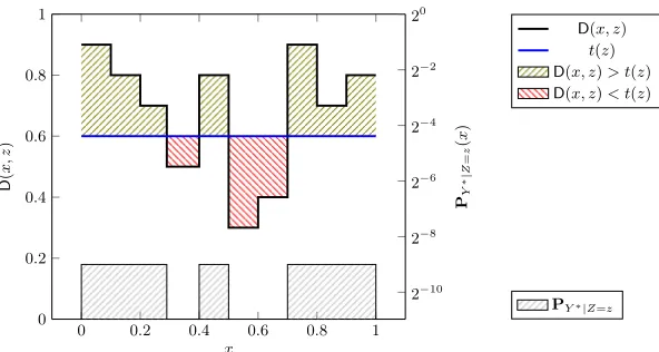
Remark 2. The characterization can be illustrated in an easy and elegant way. First, it says that the area under the graph ofD(x, z) and above the threshold t(z) is the same, no matter whatz is (see Figure3).
0 0.2 0.4 0.6 0.8 1 0
0.5 1
x
D
(
x,
z1
)
D(x, z1)
t(z1) D(x, z1)> t(z1)
0 0.2 0.4 0.6 0.8 1 0
0.5 1
x
D
(
x,
z2
)
D(x, z2)
t(z2) D(x, z2)> t(z2)
Fig. 3.For everyz, the (green) area under D(·, z) and abovet(z) equalsλ
0 0.2 0.4 0.6 0.8 1 0
0.2 0.4 0.6 0.8 1
x
D
(
x,
z
)
D(x, z) t(z)
D(x, z)> t(z)
D(x, z)< t(z)
2−10
2−8
2−6
2−4
2−2
20
PY
∗|
Z
=
z
(
x
)
PY∗|Z=z
Fig. 4.Relation between distinguisherD(x, z), thresholdt(z) and distributionY∗|Z=
z.
Note that because of “freedom” in defining the distribution on elementsx satis-fyingD(x, z) =t(z) (2, point (b)), there could be many distributions Y∗|Z cor-responding to fixed numbersλandt(z) that satisfy the characterization above, and this way are optimal to (20) with k = He∞(Y∗|Z). For the sake of com-pleteness we characterize bellow the all possible values ofkthat match toλand t(z). We note that this fact might be used to modify our nonuniform guessing algorithm into a uniform one.
Corollary 1. Let D:{0,1}n× {0,1}m→[0,1]andλ∈(0,1). Lett(z) =t(λ, z) be the unique numbers that satisfy the condition (a) in Lemma 2. Define
k(λ) =n−log (Ez←Z[1/P(D(U, z)>t(z))]), (21) which is a non-decreasing right continuous function ofλ. Letk−(λ) = limλ0→λ−k(λ0)
andk+(λ) = lim
λ0→λ+k(λ0) =k(λ)be the one-sided limits. Then for everyY∗|Z of min-entropy k=He∞(Y∗|Z)fulfilling (b),(c) and (d) we have k− 6k6k+. Conversely, if k satisfies k− 6 k 6 k+ then there exists a distribution Y∗|Z fulfilling (b),(c) and (d) such thatHe∞(Y∗|Z) =k.
Predicting given the thresholds t(z). We use the numberst(z) to modifyDand then we call the procedurePredictor on the modified distinguisher. Lemma 3 below shows that we could efficiently predictX fromZ, assuming we knew the numbers t(z) for all z in the support ofZ (later, we’ll show how to efficiently approximate them)
Lemma 3. Let Y∗|Z be the distribution satisfying He∞(Y∗|Z) = k and maxi-mizingED(Y, Z)overHe∞(Y|Z)>k, wherek < nandDsatisfies (19). Lett(z) be as in Lemma 2. Define
and set`= 2·2n−k−1 in the algorithm
Predictor. Then we have
Pr (Predictor(Z,D0, `) =X)>2−k 1 + 2k−n
(23)
Proof. We start by calculating the probability on the left-hand side of(23)
Claim 1 For any19 D0, the algorithm Predictor outputs X givenZ=z with probability
Pr
X,Z(Predictor(Z,D
0, `) =X|Z=z) = 2−n−1g
ED0(U, z)
2
·ED0(X|Z=z, z)
(24)
whereU is uniform over{0,1}n andg is defined byg(d) =1−(1−d)`
d (sog(d)≈ 1/dfor large`)
Proof (of Claim).It is easy to observe that
Pr[Predictor(z,D0, `) =x|Predictor(z,D0, `)6=⊥] = D 0(x, z)
P
x
D0(x, z) (25)
In turn, for every roundi= 1, . . . , ` of the execution, the probability that Pre-dictorstops and outputsx0is equal to Pr[U =x0]D0(x0, z)/2 = 2−n−1D0(x0, z), the probability that it outputs anything (and thus leaves the while loop) is thus
P
x0Pr[U =x0]·
1−D0(x20,z)= 1−ED0(U,z)
2 . So the probability of not leaving the while loop for `rounds (in this case the output is⊥) is
Pr[Predictor(z,D0, `) =⊥] = 1−
1−ED 0(U, z)
2
`
(26)
Combining the last two formulas we obtain
Pr[Predictor(z,D0) =x] = 2−n−1g(ED0(U, z)/2)·D0(x, z) (27) Hence
Pr[Predictor(z,D0) =X|Z =z] =X x
Pr[Predictor(z,D0) =x, X=x|Z=z]
=X
x
Pr[Predictor(z,D0) =x] Pr[X =x|Z =z]
= 2−n−1g(ED0(U, z)/2)
X
x
D0(x, z) Pr[X =x|Z =z]
= 2−n−1g(ED0(U, z)/2)ED0(X|Z=z, z) (28)
and the claim follows. ut
Now we can see why we cannot apply the algorithmPredictorusing the distin-guisherDsatisfying only (19) directly. According to the last formula, the success probability would be an averaged sum of productsg(ED(U, z))·ED(X|Z=z, z) over z. We know the average of the second factors of these products, but in general cannot compare the values ofED(U, z) for differentz’s. The crucial
ob-servation is that the distinguisher D0 we defined satisfies the same inequality (19) as D (though, D0 has the range [0,2] not [0,1] as D). Moreover D0 has a special form which allows us to simplify expression (23). The details are given in the next two claims
Claim 2 We haveED0(X, Z)−ED0(Y, Z)> for allY|Z : He∞(Y|Z)>k
Proof (of Claim). We argue that (a): ED0(X, Z)−ED0(Y∗, Z) > ED(X, Z)−
ED(Y∗, Z) and (b):Y∗|Z maximizesD0(Y, Z) overHe∞(Y|Z)>k. For the proof of (a), observe that by (22) we haveD0(x, z)>D(x, z)−t(z) for every xandz. HenceED0(X, Z)>ED(X, Z)−t(z). Moreover, ifD(x, z)−t(z)<0 then Lemma 2 impliesPY∗|Z=z(x) = 0 and thus ED0(Y∗|Z =z, z) =ED(Y∗|Z =z)−t(z).
Hence, for allz we have
ED0(X|Z =z)−ED0(Y∗|Z=z, z)>ED(X|Z=z, z)−ED(Y∗|Z=z, z)
The proof of (a) follows now by taking the average over z. The proof of (b) follows by observing that D0 satisfies the characterization in (2) witht(z) = 0
for allz. ut
Claim 3 The exists a numberλ0∈(0,1) such that ED0(U, z) =λ0 for everyz.
Proof. Lemma 2impliesP
xD
0(x, z) =λfor everyz. We can defineλ0 = 2−nλ and then it remains to showλ <2n andλ >0. Observe that the caset(z)<0 in Lemma 2 is possible if and only if PY∗|Z=z(x) = maxx0PY∗|Z=z(x0) for all x, which meansH∞(Y∗|Z =z) =n. Since k < n, we havet(z)>0 for at least one z and then λ =P
xmax(D(x, z)−t(z),0) 6
P
xD(x, z) which essentially meansλ62n. Lemma2guarantees thatλ
>0 , therefore we need to show that λ6∈ {0,2n}. Observe that if λ= 0 then the conditionP
xD0(x, z) =λimplies D0(x, z) = 0 for all xand z, contradicting to Claim 2 because > 0. In turn, if λ = 2n then from Lemma 2 we get D(·, z) ≡ 1 and t(z) = 0 for all z such thatt(z)>0. This is possible only ifPY∗|Z=z(x) = maxx0PY∗|Z=z(x0) for allx which meansH∞(Y∗|Z =z) =n ift(z)>0. But then H∞(Y∗|Z =z) =nfor
allzwhich contradictsk < n. ut
To calculate the success probability we need one more observation. The following claim shows that support ofD0 is contained in the support ofY∗.
Claim 4 For everyz we have
ED0(Y∗|Z=z, z) =ED0(U, z)·2nmax
x0 PY∗|Z=z(x
Proof (of Claim).By Lemma2,D(x, z)> t(z) only ifPY∗|Z=z(x) = maxx0PY∗|Z=z(x0) therefore
ED0(Y∗|Z =z, z) =
X
x
max(D(x, z)−t(z),0)PY∗|Z=z(x)
=X
x
max(D(x, z)−t(z),0) max
x0 PY∗|Z=z(x
0),
and the claim follows by the definition ofD0. ut
Now we are ready to prove the main result. From Claim1and Claim3we obtain
Pr (Predictor(Z,D0, `) =X) = 2−n−1Ez←Z[g(λ0/2)·D0(X|Z=z, z)] = 2−n−1g(λ0/2)·ED0(X, Z) (30) Claim2 applied toY =Y∗ yields now the following estimate
Pr (Predictor(Z,D0, `) =X)>2−n−1g(λ0/2)·(ED0(Y∗, Z) +). (31) Observe that Claim4, Claim 3, andHe∞(Y∗|Z) =kimply
ED0(Y∗, Z) =Ez←Z[D0(Y∗|Z=z, z)] =Ez←Z
h
ED0(U, z)·2nmax
x0 PY∗|Z=z(x
0)i
= 2nλ0·Ez←Z
h
max
x0 PY∗|Z=z(x
0)i= 2n−kλ0 (32)
Plugging this into (31) we get the following bound
Pr (Predictor(Z,D0, `) =X)>2−n−1g(λ0/2)· 2n−kλ0+ = 2−k 1−(1−λ0/2)`
1 + 2 k−n−1
λ0/2
(33)
To give a lower bound on the success probability it remains to minimize the last expression overλ0∈(0,1). This is answered below
Claim 5 Let h(s) = (1−(1−s)`)(1 +as−1), where a > 0 and ` >1 +a−1. Thenh(s)>h(1) = 1 +afor alls∈[0,1].
Proof (of Claim).The proof uses standard calculus and is given in the appendix. u t
Computing t(z) from λ So far, we have shown how to construct the predict-ing algorithm provided that we are given the numbers t(z). Now we will prove that one can compute themapproximately and usesuccessfully in place of the original ones. We start with a few useful facts about the auxiliary function g already introduced in Claim1in the proof of Lemma3. Below we summarize its fundamental properties.
(a) g is continuous at 0 and decreasing (b) g is convex
(c) for anyd2> d1 we have g(d2)> g(d1) 1−2`· |d2−d1|
Proof (of Lemma). The proof uses elementary calculus and is referred to the
appendix ut
The entire solution is based on the next two lemmas. The first lemma is based on the intuition that replacingDby a distinguisher which approximates it close enough should not affect the success probability of Predictor(Z,D, `) very much. For technical reasons we present this statement assuming one-sided L1 -approximation. The second lemma describes an efficient algorithm which obtains λas a hint on its input and computes approximations fort(z) from below, for every z.
Lemma 5. LetD1,D2:{0,1}n×{0,1}m→[0,1]be any two functions satisfying (a) D2(x, z)>D1(x, z) for allx, z
(b) ED2(U, z)−ED1(U, z)6δfor all z Then we have
Pr (Predictor(Z,D2, `) =X)>(1−`δ/2) Pr (Predictor(Z,D1, `) =X) (34)
Proof (of Lemma). We have
Pr (Predictor(z,D2, `) =X|Z=z) =g(ED2(U, z))ED2(X|Z =z, z) >g(ED2(U, z))ED1(X|Z =z, z), (35)
where the inequality follows from D2 >D1 > 0. The assumptions (a) and (b) imply|ED1(U, z)−ED2(U, z)|6δfor everyz. From property (c) in Lemma4it
follows that
g(ED2(U, z))>g(ED1(U, z))(1−`δ/2)
for everyz. Combining the last two estimates we get
Pr (Predictor(z,D2, `) =X|Z=z)>(1−`δ/2)·g(ED1(U, z))ED1(X|Z=z, z)
= (1−`δ/2)·Pr (Predictor(z,D1) =X|Z=z) (36)
Taking the average overz←Z completes the proof. ut
Lemma 6. Let D : {0,1}n → [0,1] be any function computable in time s, let λ∈ (0,1) and t ∈[0,1]be a number such that Emax(D(U)−t,0) = λ. There exists a probabilistic algorithm FindThreshold(D, λ, δ, N) that runs in time O(log(1/δ)N·time(D))and with probability at least1−2 log(12/δ)e−N δ2/3
FunctionFindThreshold(D, λ, δ, N)
Input :D:{0,1}n→[0,1],λ∈(0,1), parametersδ, N Output:t0such thatEmax(D(U)−t0,0)∈[λ, λ+δ]
1 t−← −1, t+←1 2 repeat
3 t0←(t−+t+)/2
4 x1, . . . , xN←U /* fresh values every time */
5 λ0←N−1PjN=1max (D(xj)−t0,0) /* λ0≈Emax(D(U)−ti,0) */
6 if λ0> λ+23δ then
7 t−←t0
8 else if λ0< λ+δ3 then
9 t+←t0
10 else
11 returnt0
12 end
13 until t+−t−6 12δ 14 if t0<−1 +12δ then 15 t0← −1
16 returnt0
Proof (of Lemma). The idea is pretty simple: given t0 we approximate values
Emax(D(U)−t0,0) by sampling and by comparing the result with λ, we can
find the right value oft0 using binary search. This corresponds to finding a blue line on Fig.4such that the green area above is sufficiently close toλ.
The functionh(t0) =Emax(D(U)−t0,0) is clearly non-increasing with respect
to t0 and changes from 1 +ED(U) at t0 = −1 to 0 for t = 1. Moreover, it is
strictly decreasing in a small neighborhood of t0 =t and for all t0 < t. Indeed, since λ > 0 there is at least one x such that D(x) > t. Taking t0 < t00 6 minx:D(x)>tD(x) we see that h(t0)−h(t00) > 2−n(t00−t0) > 0. Hence, t0 > t implies Emax(D(U)−t0,0) <Emax(D(U)−t,0) =λ. This proves the second part of the statement. Denote byλ0i, t0i, t−i , t+i the values assigned in round i to λ0, t0, t−, t+ respectively. Observe that by the Chernoff Bound20 and the union bound over at most log(12/δ) rounds of the execution, with probability p = 1−2 log(12/δ) exp(−N δ2/3) we have |λ0
i−h(ti)| < 12δ for every round i. Note that with the same probability the algorithm satisfies the invariant property: if there ist0∈[t−i , t
+
i ] such thath(t0)∈λ+5δ12, λ+7δ12and the algorithm jumps to round i+ 1 then t0 ∈
t−i+1, t+i+1. Suppose that h(t0)∈
λ+5δ12, λ+7δ12 for somet0∈[−1,1]. Now we have two possibilities: either we terminate withtisuch thatλi∈
λ+δ3, λ+2δ3which meansh(ti)∈
λ+3δ12, λ+7δ12and we are done, or we will eventually find sucht0up to an error12δ . Since|h(t2)−h(t1)|6|t2−t1| for any t1, t2, the returned number t0 satisfies h(t0)−12δ 6h(t0)6h(t0) + 12δ , in particular it satisfies the desired inequality. It remains to consider the case
20We use the following version: letX1, . . . , X
N be [0,1]-valued independent random
variables, letX =PN
when eitherh(t)< λ+5δ
12 for alltorh(t)> λ+ 7δ
12. Sinceh(1) = 0 the second is clearly impossible. In the first case we haveh(t)6h(−1)< λ+5δ12, which means that in every roundiwe havet−i =−1 and either we terminate withti such that λ0i ∈
λ+δ3, λ+2δ3which means h(ti)∈
λ+3δ12, λ+7δ12and we are done, or in every roundiwe do the assignmentt+i+1=tiwhich yieldsti=−1+2−i+1and the main loop halts with ti <−1 +12δ. The algorithm outputs then−1 which satisfies the desired inequality, because of the assumptionh(−1) < λ+5δ12 and
the trivial inequalityh(−1)>1>λ. ut
Let D0 be as in Lemma 3. Let t0(z) =
FindThreshold(D, λ, δ, N), define D00(x, z) = max(D(U, z)−t0(z),0). Denote by Pr[bad] the probability thatED00(U, z)6∈ [λ, λ+δ] (i.e. probability of failure of the algorithmFindThreshold). If the event bad doesn’t occur then D00 >D0 and ED00(U, z)6ED0(U, z) +δ. Applying the last two claims we obtain
Pr [Predictor(z,D00, `)]>2−k 1 + 2k−n
·
1−`δ 2
Pr[¬bad] (37)
By the elementary inequality (1 +s)(1−s/4)2
>1 valid fors ∈[0,1], for this probability to be bigger than 2−k it is enough to require
`δ/262k−n/4 (38) 2 log(12/δ) exp(−N δ2)/3)62k−n/4 (39) The solution for the first inequality isδ=O(22(k−n)2) which impliesδ. The second one gives us N = Ω (1/δ)2(log log(1/δ) +n−k+ log(1/)
which can be simplified toN =Ω (1/δ)2(log(1/δ)
. The total running time is (up to a con-stant factor) the time needed for invokingO(`·Nlog(1/δ)) =O (2∆/)5log2 2∆/ times of the distinguisherD.
D
Proof of Lemma
2
Proof. Consider the following linear optimization program
maximize Px,z,az
X
x,z
D(x, z)P(x, z)
subject to −Px,z60, (x, z)∈ {0,1}n× {0,1}m
X
x
Px,z−PZ(z) = 0, z∈ {0,1}m
Px,z−az60, z∈ {0,1}m
X
z
az−2−k60
(40)
This problem is equivalent to (20) if we definePY,Z(x, z) =P(x, z) and replace the condition P
zmaxxPY,Z(x, z)62
−k, which is equivalent to
e
Claim 6 The numbers(Px,z)x,z,(az)z are optimal for (40) if and only if there exist numbersλ1(x, z)
>0,λ2(z)∈
R,λ3(x, z)>0,λ4>0such that
(a) D(x, z) =−λ1(x, z) +λ2(z) +λ3(x, z)and0 =−P
xλ
3(x, z) +λ4
(b) We have λ1(x, z) = 0 if Px,z > 0, λ3(x, z) = 0 if Px,z < az, λ4 = 0 if
P
zaz<2−k.
Proof (of Claim).This is a straightforward application of KKT conditions. ut
It remains to apply and simplify the last characterization. Let (Px,z∗ )x,z,(a∗z)z be optimal for (40), whereP∗(x, z) =PY∗,Z(x, z), andλ1(x, z), λ2(z), λ3(x, z), λ4(x) be corresponding multipliers given by the last claim. Define t(z) = λ2(z) and λ =λ4. Observe that for every z we have a∗
z >maxx P(x, z)> 2−nPZ(z)>0 and thus for every (x, z) we have
λ1(x, z)·λ3(x, z) = 0 (41)
If P∗(x, z) = 0 then P∗(x, z) < a∗(z) and λ3(x, z) = 0, hence D(x, z) 6 t(z) which proves (c). IfP∗(x, z) = maxx0P∗(x, z) thenP∗(x, z)<0 andλ1(x, z) = 0
which proves (d). Finally observe that (41) implies
max(D(x, z)−t(z),0) = max(−λ1(x, z) +λ3(x, z),0) =λ3(x, z) Hence, the assumptionP
xλ
3(x, z) =λ4=λproves (a).
Suppose now that the characterization given in the Lemma is satisfied. Define P∗(x, z) =PY,Z(x, z) andaz = maxzPY∗,Z(x, z), letλ3(x, z) = max(D(x, z)− t(z),0), λ1(x, z) = max(t(z)−D(x, z),0) and λ4 =λ. We will show that these numbers satisfy the conditions described in the last claim. By definition we have −λ1(x, z) +λ2(z) +λ3(x, z) =D(x, z), by the assumptions we getP
xλ
3(x, z) = λ = λ4. This proves part (a). Now we verify the conditions in (b). Note that D(x, z)< t(z) is possible only if PY∗|Z=z(x) = 0 and D(x, z)> t(z) is possible only if PY∗|Z=z(x) = maxx0PY∗|Z=z(x0). Therefore, ifPY,Z(x, z)>0 then we must haveD(x, z)>t(z) which means thatλ1(x, z) = 0. Similarly ifPY,Z(x, z)< maxzPY∗,Z(x, z) thenD(x, z)6t(z) andλ3(x, z) = 0. Finally, since we assume
e
H∞(Y∗|Z) =kwe havePzaz= 2
−k and thus there is no additional restrictions
onλ4. ut
E
Proof of Corollary
1
Proof (of Corollary).Letymax(z) = maxx0PY|Z=z(x0). Consider the function
fzδ(x) =
ymax(z) +δ,D0(x, z)> t(z) 1−#{x: D0(x.z)>t(z)}·(ymax+δ)
#{x: D0(x,z)=t(z)} ,D0(x, z) =t(z) 0,D0(x, z)< t(z)
(42)
This function defines a distribution that satisfies
fzδ(x)6max x0 f
δ z(x
0) ∀x:D0(x, z)