Nonlinearity of the forward-backward correlation function in the model with string fusion

Nonlinearity of the forward-backward correlation function in the

model with string fusion

Vladimir Vechernin1,

1_{Saint Petersburg State University, 7/9 Universitetskaya nab., St.Petersburg, 199034 Russia}

Abstract. The behavior of the forward-backward correlation functions and the corre-sponding correlation coefficients between multiplicities and transverse momenta of

par-ticles produced in high energy hadronic interactions is analyzed by analytical and MC calculations in the models with and without string fusion. The string fusion is taking into account in simplified form by introducing the lattice in the transverse plane. The results obtained with two alternative definitions of the forward-backward correlation co-efficient are compared. It is shown that the nonlinearity of correlation functions increases

with the width of observation windows, leading at small string density to a strong de-pendence of correlation coefficient value on the definition. The results of the modeling

enable qualitatively to explain the experimentally observed features in the behavior of the correlation functions between multiplicities and mean transverse momenta at small and large multiplicities.

1 Introduction

The investigations of long range rapidity correlations give the information about the initial stage of high energy hadronic interactions [1]. In paper [2] the study of the correlations between multiplicities in two separated rapidity windows (the long range forward-backward correlations) to find a signature of the string fusion and percolation phenomenon [3–6] in ultrarelativistic heavy ion collisions has been proposed. Later it was realized [7–12] that the investigations of the forward-backward correlations involving intensive observables, such e.g. as the event-mean transverse momentum, enable to obtain more clear signal about the initial stage of hadronic interaction, including the process of string fusion, compared to usual forward-backward multiplicity correlations.

In the present work, correlation functions and correlation coefficients between the observables in two separated rapidity intervals in ultrarelativistic heavy ion collisions are analyzed by analytical and MC calculations in a simple model which enables to take into account the string fusion effects. It is shown that the nonlinearity of correlation function increases with the width of observation windows, leading at small string density to the strong dependence of correlation coefficient value on the defini-tion. Whereas the forward-backward correlation function itself is uniquely defined and carries more physical information than the correlation coefficients deduced from it.

2 Definitions

The forward-backward (FB) correlation function, for the correlation between two observables,Fand B, measured event-by-event in rapidity intervals,δηF andδηB, separated by some rapidity gap,ηgap, gives the dependence of the mean value of the variableBon the variableF:

BF = f(F), (1)

In present paper we restrict ourself to the study of long range FB correlations between the multiplici-ties of charged particles (n-n) and between the event-mean transverse momentum and the multiplicity (pt-n). So asFwe use the multiplicity of charged particles,nF, measured in forward rapidity window and asBwe use the multiplicity of charged particles,n_B, measured in backward rapidity window or the event-mean transverse momentum of these particles,p_B:

pB=_n1 B

nB

i=1

|pi

tB|. (2)

In the last case of the pt-n correlation we expect smaller influence on results of the trivial fluctua-tions in the number of sources (strings) - the so called “volume” fluctuafluctua-tions. Being an intensive variable, thepB does not depends directly on the number of strings. It is sensitive to changes in the characteristics of the sources, e.g. due to the string fusion processes.

Usually the strength of the FB correlation is characterized by the correlation coefficientbFB. Un-fortunately the definition of the correlation coefficient is not unique (see e.g. [13] for a review). One of the most popular definition [14, 15] is

bFB= FB − FB

F2 _{− F}2 =

cov(F,B)

DF . (3)

Another possible option [8, 9]:

b

FB= dBF

dF

_F=F . (4)

In the case of an integer variableF, asn_F, one has to interpret this definition as follows

b

FB=B[F]− B[F]+1, (5)

where the [F] is an entire part of theF. It is clear that the definitions ofbFBandbFBare the same for the linear correlation function

BF =a+bFBF, (6)

the so-called linear regression, differing from each other in the general case.

2 Definitions

The forward-backward (FB) correlation function, for the correlation between two observables,Fand B, measured event-by-event in rapidity intervals,δηF andδηB, separated by some rapidity gap,ηgap, gives the dependence of the mean value of the variableBon the variableF:

BF = f(F), (1)

In present paper we restrict ourself to the study of long range FB correlations between the multiplici-ties of charged particles (n-n) and between the event-mean transverse momentum and the multiplicity (pt-n). So asFwe use the multiplicity of charged particles,nF, measured in forward rapidity window and asBwe use the multiplicity of charged particles,n_B, measured in backward rapidity window or the event-mean transverse momentum of these particles,p_B:

pB= _n1 B

nB

i=1

|pi

tB|. (2)

In the last case of the pt-n correlation we expect smaller influence on results of the trivial fluctua-tions in the number of sources (strings) - the so called “volume” fluctuafluctua-tions. Being an intensive variable, the pB does not depends directly on the number of strings. It is sensitive to changes in the characteristics of the sources, e.g. due to the string fusion processes.

Usually the strength of the FB correlation is characterized by the correlation coefficientbFB. Un-fortunately the definition of the correlation coefficient is not unique (see e.g. [13] for a review). One of the most popular definition [14, 15] is

bFB=FB − FB

F2 _{− F}2 =

cov(F,B)

DF . (3)

Another possible option [8, 9]:

b

FB= dBF

dF

_F=F . (4)

In the case of an integer variableF, asn_F, one has to interpret this definition as follows

b

FB=B[F]− B[F]+1, (5)

where the [F] is an entire part of theF. It is clear that the definitions ofbFBandbFBare the same for the linear correlation function

BF =a+bFBF, (6)

the so-called linear regression, differing from each other in the general case.

Due to the locality of strong interaction in rapidity the FB correlation naturally divides into two parts: the short- and the long-range ones. The short-range correlation takes place only between par-ticles produced from a same source (string). It goes to zero for large enough rapidity gaps,ηgap 2. The origin of the long-range correlations at largeηgapis event-by-event variance in the number and properties of particle sources (strings [13], cut pomerons [16] and so on), formed in high energy hadronic interaction. In present paper we will consider only these long-range part of the correlations, as we are interested in the study of the variations in number and properties of the strings, produced at the initial stage of the hadronic interaction.

3 The model

We will take into account the string fusion effects in simplified form by introducing a lattice in the transverse plane. This discrete version of string fusion model [5, 6] was introduced in [17] and then was exploited for a description of various phenomena (correlations, anisotropic azimuthal flows, the ridge) in high energy hadronic collisions [8–12, 19–21]. In this approach one splits the impact parameter plane intoM cells with the area equal to the transverse area of single string, σstr, and supposes the fusion of all strings with the centers in a given cell. Then each string configuration is characterized by the set of integers:

Cη={η1, ..., ηM} , (7)

whereηiis a number of initial strings fused in a giveni-th cell . This leads to the splitting of the transverse area into domains with different, fluctuating values of color field within them. What is similar to the attempts to take into account the density variation in transverse plane in models based on the BFKL evolution [22] and on the CGC approach [23].

In this model one supposes that theηiin each cell fluctuates around the same mean valueηwith a scaled varianceωη. Then in accordance with the string fusion prescription [5, 6] the mean number of

charged particles in forward and backward observation windows, produced from the fragmentation of fused strings in thei-th cell, is given by the expression

nFi =µF√ηi, nBi =µB√ηi, (8)

whereµFis a mean number of particles produced from decay of a single string in the forward window

δηF. Clear thatµF is proportional to the window width: µF =µ0δηF and the same for the backward window. Note that in the framework of the present model we can simultaneously calculate the results without taking into account the string fusion effects simply using instead of (8) the dependencen_iF = µFηi.

Because we study only LRC, we also suppose the independent fragmentation of thei-th fused string in forward and backward windows. So the corresponding numbers of charge particlesnF

i and nB

i fluctuates independently event-by-event around the above mean values with some scaled variance

ωµ.

Finally, in accordance with the string fusion ideas [5, 6] we suppose that the transverse momentum distribution of particles, produced from theηifused strings, has enlarged mean transverse momentum:

p(ηi)=p0√4ηi, (9)

wherep0is a mean transverse momentum for particles produced from a decay of a single string. Basically in this model one can calculate the correlation functions and the correlation coefficients by direct MC simulations using the definitions (1)-(5). To calculate n-n correlation one needs to generate the following configuration

C=Cη,CnF,CnB

, (10) where CF n = nF 1, ...,nFM

, CB

n =

nB 1, ...,nBM

. (11)

HerenF

i andnBi are the numbers of charged particles, produced in forward and backward windows from the fragmentation of fused string ini-th cell. Forpt-ncorrelation one needs also to generate the transverse momentap_tijBof allnB

i particles produced in backward window for each cell:

CB p =

p1B t1, ...,p

nB 1B

t1 ;...;p1tMB, ...,p nB

MB tM

supposing some transverse momentum distribution in accordance with (9). The physical observables, defined in previous Sect. 2, are expressed through these generated values:

nF = M

i=1 nF

i , nB= M

i=1 nB

i , pB= 1 n_B

M

i=1 nB

i

j=1

p_tijB. (13)

As we will see below such direct MC approach to the calculation of the correlation functions and coefficients in not optimal. The approach, in which part of the computations is performed analytically, proves to be more practical. It allows considerably reduce the amount of MC simulations, enabling more precise results for the correlation function in the regions of very small or large multiplicityn_F. Whereas the direct MC approach needs a huge number of simulations to generate configurations with n_F, which is considerably different fromn_F.

These simplifying analytical calculations we will perform using the representation for the long-range FB correlation function, exploited in [15]:

BF =

CBCP(C)PC(F)

CP(C)PC(F) , (14)

whereP(C) is the probability of realization of the configurationC in a given event. TheBC and PC(F) are correspondingly, the mean value of the observable B in the backward window and the probability to have the valueFfor the observable in the forward window for given configurationC.

4 Correlation between multiplicities

In paper [17] the non-monotonic dependence of the correlation coefficientsb_nn andb_ptn on string densityηat small string densities was found. What is interesting the effect took place only for the extended rapidity windows. We start the analysis of this effect from the consideration of then-n correlation. In this case at small string density as a first step we can neglect string fusion and check whether there is this effect without a string fusion.

4.1 The correlation coefficientbnn

In the version of the model without string fusion the allocation of strings on cells does not play any role and the configurationCηis characterized simply by the total number of strings:

N=

M

i=1

ηi. (15)

In this case, acting as in [24], we can obtain the explicit analytical formula forbnn, (3):

bnn = ωN−λN

ωµF/µF+ωN−λN

, (16)

whereωµFandωNare the corresponding scaled variances:

ωµF =DµF/µF, ωN=DN/N =ωη, DN =N2−N 2

, N=ηM (17)

and

supposing some transverse momentum distribution in accordance with (9). The physical observables, defined in previous Sect. 2, are expressed through these generated values:

nF = M

i=1 nF

i , nB= M

i=1 nB

i , pB= 1 n_B

M

i=1 nB

i

j=1

p_tijB. (13)

As we will see below such direct MC approach to the calculation of the correlation functions and coefficients in not optimal. The approach, in which part of the computations is performed analytically, proves to be more practical. It allows considerably reduce the amount of MC simulations, enabling more precise results for the correlation function in the regions of very small or large multiplicityn_F. Whereas the direct MC approach needs a huge number of simulations to generate configurations with n_F, which is considerably different fromn_F.

These simplifying analytical calculations we will perform using the representation for the long-range FB correlation function, exploited in [15]:

BF =

CBCP(C)PC(F)

CP(C)PC(F) , (14)

whereP(C) is the probability of realization of the configurationC in a given event. TheBC and PC(F) are correspondingly, the mean value of the observable B in the backward window and the probability to have the valueFfor the observable in the forward window for given configurationC.

4 Correlation between multiplicities

In paper [17] the non-monotonic dependence of the correlation coefficients b_nn andb_ptn on string densityηat small string densities was found. What is interesting the effect took place only for the extended rapidity windows. We start the analysis of this effect from the consideration of the n-n correlation. In this case at small string density as a first step we can neglect string fusion and check whether there is this effect without a string fusion.

4.1 The correlation coefficientbnn

In the version of the model without string fusion the allocation of strings on cells does not play any role and the configurationCηis characterized simply by the total number of strings:

N=

M

i=1

ηi. (15)

In this case, acting as in [24], we can obtain the explicit analytical formula forbnn, (3):

bnn = ωN−λN

ωµF/µF+ωN−λN

, (16)

whereωµFandωNare the corresponding scaled variances:

ωµF =DµF/µF, ωN=DN/N=ωη, DN =N2−N 2

, N=ηM (17)

and

λ=P(0)/[1−P(0)], P(0)=pM(0). (18)

0 0.2 0.4 0.6 0.8 1

0 0.05 0.1 0.15 0.2 0.25 0.3 0.35 0.4 0.45 0.5

b

η

M=30 - MC M=10 - MC M=30 - analit. M=10 - analit.

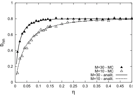
Figure 1.The FB multiplicity correlation coefficient,bnn, (3), calculated by direct MC simulations (points) and analytically by formula (21) (curves) for lattices withM =10 and 30 cells as a function ofη(theη/σstris a string density), using the wide observation windows, corresponding toµF =4. The poissonian distribution for the number of particles produced from a string (ωµF =1) and the modified (19) poissonian distribution for the

fluctuation in the number of strings were supposed. The string fusion processes are not taken into account.

Herep(0) is the probability to have zero number of string in a given cell. In addition to the considera-tion in [24] we take into account that modeling inelastic collisions we have to discard the events with zero total number of strings. This corresponds to the following simple modification (P(N)→ P_(N))

of event string distribution:

P_{(0)=0 ; P(N)=P(N)/1−P(0), N≥1. (19)}

We denote asNandNthe mean values calculated correspondingly withP(N) andP_(N).

In paper [17] the non-monotonic dependence on string density was obtained for the modified poissonian distribution of the total number of strings. In this case

P(0)=pM(0)=e−ηM=e−N, Nk_=Nk_/(1−e−N_{) (20)}

and the formula (16) converts into

bnn= 1−ληM ωµF/µF+1−ληM

, λ= e

−ηM

1−e−ηM . (21)

We see that the dependence of the correlation coefficient onMtakes place only in the regionη1/M (see figure 1). At other values ofηwe have the well known resultbnn=µF/(µF+ωµF) [25].

0 0.2 0.4 0.6 0.8 1

0 0.05 0.1 0.15 0.2 0.25 0.3 0.35 0.4 0.45 0.5

b

η

µ_F=4, with fusion - MC µ_F=4, no fusion - MC µ_F=4, no fusion - analyt. µ_F=1, with fusion - MC µ_F=1, no fusion - MC µ_F=1, no fusion - analyt.

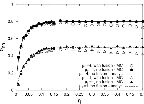
Figure 2. The same as in figure 1, but for the two widths of observation windows,µF =1 and 4, for the lattice withM=30 cells. The open points demonstrate the influence of string fusion processes.

The analysis shows also that this decrease withηis monotonic at any value of the parameterµF, i.e. for the observation windows of arbitrary width in rapidity (see figure 2). So it can not explain the non-monotonic behavior ofb

nn observed in [17] for wide rapidity windows, correspondingµF =4. The taking into account the string fusion processes does not change the situation forbnn at small values ofη(see figure 2).

We have to suppose now that this non-monotonic behavior ofb

nnarises due to nonlinearity of the forward-backward correlation function for wide observation windows, which leads to the difference between the correlation coefficientsb_nn andb_nn, defined by (3) and (4). To calculate the correlation coefficientb_nn, we have at first to calculate the correlation functionn_Bn

F.

4.2 The correlation functionn_Bn_F

For the case without string fusion taking into account considerations of the previous subsection 4.1 we can present the formula (14) as

BF =

N=1BNP(N)PN(F)

N=1 P(N)PN(F) , (22)

with

BN =µBN, FN =µFN. (23)

In this subsection to be short we imply thatF = n_F andB =n_B, but do not fulfill this substitution explicitly. As in paper [17] we will suppose the poissonian distribution for charge particles from a string decay. Then the distribution from decay ofNstring also will be poissonianPN(F):

0 0.2 0.4 0.6 0.8 1

0 0.05 0.1 0.15 0.2 0.25 0.3 0.35 0.4 0.45 0.5

b

η

µ_F=4, with fusion - MC µ_F=4, no fusion - MC µ_F=4, no fusion - analyt. µ_F=1, with fusion - MC µ_F=1, no fusion - MC µ_F=1, no fusion - analyt.

Figure 2. The same as in figure 1, but for the two widths of observation windows,µF =1 and 4, for the lattice withM=30 cells. The open points demonstrate the influence of string fusion processes.

The analysis shows also that this decrease withηis monotonic at any value of the parameterµF, i.e. for the observation windows of arbitrary width in rapidity (see figure 2). So it can not explain the non-monotonic behavior ofb

nn observed in [17] for wide rapidity windows, correspondingµF =4. The taking into account the string fusion processes does not change the situation for bnn at small values ofη(see figure 2).

We have to suppose now that this non-monotonic behavior ofb

nnarises due to nonlinearity of the forward-backward correlation function for wide observation windows, which leads to the difference between the correlation coefficientsb_nn andb_nn, defined by (3) and (4). To calculate the correlation coefficientb_nn, we have at first to calculate the correlation functionn_Bn

F.

4.2 The correlation functionn_Bn_F

For the case without string fusion taking into account considerations of the previous subsection 4.1 we can present the formula (14) as

BF =

N=1BNP(N)PN(F)

N=1 P(N)PN(F) , (22)

with

BN =µBN, FN =µFN. (23)

In this subsection to be short we imply thatF = n_F andB = n_B, but do not fulfill this substitution explicitly. As in paper [17] we will suppose the poissonian distribution for charge particles from a string decay. Then the distribution from decay ofNstring also will be poissonianPN(F):

PN(F)=e−µFN(µFN)F/F!, (24)

0 10 20 30 40 50

0 10 20 30 40 50 60 70 80

<n

>

n

η

=0.01

MC analit. <nF>

0 10 20 30 40 50

0 10 20 30 40 50 60 70 80

<n

>

n

η

=0.04

MC analit. <nF>

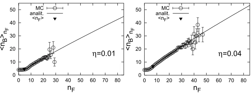
Figure 3.The correlation function between the multiplicities of charged particles produced in the backward,n_B, and forward,n_F, rapidity intervals at string densities, correspondingη=0.01 (left panel) andη=0.04 (right panel), for large observation windows withµF=4. The points are the results obtained in the model on the base

of 800 000 direct MC simulations, the curves are obtained by the analytical calculations using formulas (25) and (29). The black triangular marks the mean valuenF.

Substituting in (22) we get:

BF =µBΦ(F+1)

Φ(F) , Φ(F)≡

N=1

P(N)NF_e−µFN_{. (25)}

This result is in agreement with the formulaBF =(F+1)P(F+1)/P(F), obtained using generating function technique for the caseµF =µB in [15]. Note the nonlinear dependence of the correlation function onµF.

If we will use as in the previous subsection 4.1 and in paper [17] the modified poissonian distri-butionP_{(N) for the total number of strings, then omitting common constant factor, we can use as} Φ(F)

Φ(F)=

N=1

NFaN

N! =

ad da

F

ea_{, F≥1, (26)}

Φ(0)=ea−1, a≡Ne−µF _=ηMe−µF ₍₂₇₎

for the calculation ofBFin (25). By (26) we can get explicit expression:

Φ(F)=ea

F

k=1

(−1)k_ak

k!    k m=1

(−1)m_Cm kmF

 

 . (28)

But practical calculations by the formula (28) is not convenient, as the sum is alternating. More suitable to use the following recurrence relation:

Φ(F)=eaSF, SF =

F

k=1

b(_kF)ak_{, F≥1, (29)}

0 0.2 0.4 0.6 0.8 1

0 0.05 0.1 0.15 0.2

b’

, b

η

b’_nn - MC by derivative b’_nn - analit. by derivative b_nn - MC by correlator bnn - analit. by correlator

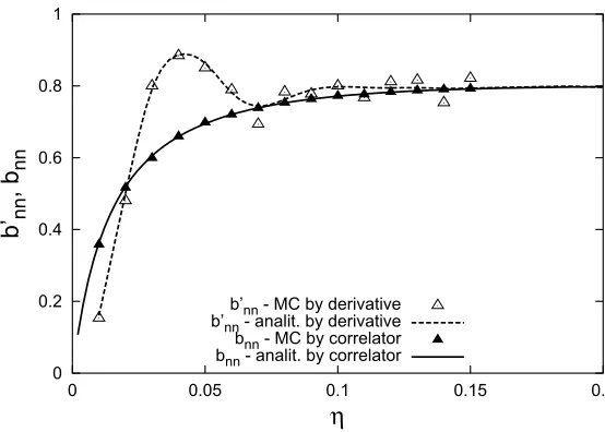
Figure 4.The comparison of the FB correlation coefficientsbnn(filled points, solid curve) andbnn(open points, dash curve), defined by (3) and (4), as a function of string density. The points are the results of direct 800 000 MC simulations, the curves are analytically calculated using the formulas (21), (25) and (29).

The results of the calculation of the correlation functionn_Bn_Fby these analytical formulae and by direct MC simulations are presented in figure 3. We see the good agreement and that the analytical approach enables to calculate the FB correlation function at large multiplicitiesn_F, when direct MC simulations can not produce a result even after 800 000 simulations.

4.3 The correlation coefficientb

nn

Now by (5) we can calculate the correlation coefficientb_nn. The results obtained by analytical cal-culations and by direct MC simulations are presented in figure 4. We see that even without string fusion for wide rapidity windows (µF =4) we have the non-monotonic behavior ofbnnat small string density, observed in [17].

We can understand the origin of this non-monotonic behavior ofb

nncomparing the left and right panel plots in figure 3. In these plots we have marked the pointn_F, in which the correlation coeffi -cientb

nn is calculated. We see that with the increase ofηthe form of the correlation functionnBnF remains almost unchanged, whereas the pointn_Fmoves to higher values. Due to nonlinearity of the correlation functionn_BnFat small values ofnF this leads to the non-monotonic behavior ofb

nnwith the increase ofη.

The detail analysis shows that this nonlinearity at small values ofn_Farises only for the observation windows which are wide in rapidity e.g. it takes place atµF =4 and does not take place atµF =1. The reason is that for wide rapidity windows the contributions to the correlation functionn_BnFfrom configurations with one and two strings are not almost overlapping.

5 Correlation between transverse momentum and multiplicity

0 0.2 0.4 0.6 0.8 1

0 0.05 0.1 0.15 0.2

b’

, b

η

b’_nn - MC by derivative b’_nn - analit. by derivative b_nn - MC by correlator bnn - analit. by correlator

Figure 4.The comparison of the FB correlation coefficientsbnn(filled points, solid curve) andbnn(open points, dash curve), defined by (3) and (4), as a function of string density. The points are the results of direct 800 000 MC simulations, the curves are analytically calculated using the formulas (21), (25) and (29).

The results of the calculation of the correlation functionn_Bn_F by these analytical formulae and by direct MC simulations are presented in figure 3. We see the good agreement and that the analytical approach enables to calculate the FB correlation function at large multiplicitiesn_F, when direct MC simulations can not produce a result even after 800 000 simulations.

4.3 The correlation coefficientb

nn

Now by (5) we can calculate the correlation coefficientb_nn. The results obtained by analytical cal-culations and by direct MC simulations are presented in figure 4. We see that even without string fusion for wide rapidity windows (µF =4) we have the non-monotonic behavior ofbnnat small string density, observed in [17].

We can understand the origin of this non-monotonic behavior ofb

nncomparing the left and right panel plots in figure 3. In these plots we have marked the pointn_F, in which the correlation coeffi -cientb

nn is calculated. We see that with the increase ofηthe form of the correlation functionnBnF remains almost unchanged, whereas the pointn_Fmoves to higher values. Due to nonlinearity of the correlation functionn_BnFat small values ofnFthis leads to the non-monotonic behavior ofb

nnwith the increase ofη.

The detail analysis shows that this nonlinearity at small values ofn_Farises only for the observation windows which are wide in rapidity e.g. it takes place atµF =4 and does not take place atµF =1. The reason is that for wide rapidity windows the contributions to the correlation functionn_BnF from configurations with one and two strings are not almost overlapping.

5 Correlation between transverse momentum and multiplicity

In the present model the correlations between event-mean transverse momentum p_B, (13), in the backward window and the multiplicity n_F in the forward window arises only when we take into

0.29 0.3 0.31 0.32 0.33 0.34

0 20 40 60 80 100 120

<p

>

n

analit. <n_F>

0.29 0.295 0.3 0.305 0.31 0.315 0.32 0.325 0.33

0 10 20 30 40 50 60

<p

>

n

analit. <n_F>

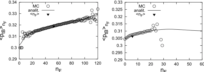
Figure 5. The function of long-range FB correlation between the event-mean transverse momentum, p_B, of particles in the backward rapidity window, (2), and the multiplicity,n_F, in the forward window, arising due to string fusion processes, for two sets of parameters:η=0.5,µF =4 (left panel) andη=0.2,µF=1 (right panel). The parameterp0 =0.3 GeV/c, the value of the mean transverse momentum for a single string in formula (9),

was chosen. The circles are the results obtained in the model on the base of 800 000 direct MC simulations, the curves are obtained by the semi-analytical calculations using formulas (32), (33) and (34). The black triangular marks the mean valuen_F.

account the string fusion process as it was explained above. We again can simplify the MC simulations performing part of the work analytically. As in the case ofn-ncorrelation, considered in Sect. 4, we start from the general formula (14):

pBn_F=

CpB_CP(C)PC(n_F)

CP(C)PC(n_F) (30)

Recall that nowC=Cη,CnF,CBn,CBp

by the remark before formula (12). Averaging of thep_B, given by the formula (13), over configurationsCB

pwe have

pB_CηCB n =

M

i=1niBp(ηi)

M i=1niB

CηCnB

, (31)

wherep(ηi) is given by (9). In paper [8] it is shown that for the poissonian distribution innB_i averaging over configurationsCB

n leads to:

ptBCη = M

i=1niB(ηi)p(ηi)

M i=1niB(ηi)

Cη

, (32)

withnB

i(ηi) given by (8) (see also [26]). After that the general formula (30) is reduced to

pBn_F=

CηpBCηP(Cη)PCη(nF)

CηP(Cη)PCη(nF)

, (33)

where for poissonian distribution innF i:

PCη(nF)=PnF(nF)=e− nFnF

n_F

n_F! , nF=µF M

i=1

√_η

The residual averaging over configurationsCηin (33) can be easily done by MC simulations.

An example of the calculation of thepBn_Fcorrelation function by this semi-analytical approach and by direct MC simulations is presented in figure 5. We see again the good agreement and that the semi-analytical approach enables to calculate the FB correlation function in wider region ofn_F, than direct MC simulations.

We would like to draw attention to an interesting detail. In right panel of figure 5 we observe the slight decrease of thept-ncorrelation function at extremely large multiplicities. One can find the signature of this effect in figure 7 in paper [27] for the correlation between transverse momentum and multiplicity of charged particles produced in the same window (in the acceptance of ALICE TPC

|η|<0.8) in 900 GeV pp collisions.

In the framework of the present model this effect has the following explanation. In events with the highest number of initial strings, the fluctuations in their distribution on transverse plane, compared to the uniform distribution, increase the event-mean transverse momentum and decrease the event multiplicity, due to string fusion effects, what leads to the negative correlation between them in this region of largen_F.

6 Concluding remarks

We have analyzed the behavior of the forward-backward correlation functions and the corresponding correlation coefficients between multiplicities and transverse momenta by analytical and MC calcu-lations in the model with a string fusion on a transverse lattice. We see that in many cases the FB correlation function,BF, occurs nonlinear, containing the physical information, which can not be reduced to the one number - the correlation coefficient. As consequence the value of the correlation coefficient in these cases can depend on its definition (e.g. bnn bnn), whereas the corresponding correlation function,n_Bn_F, is uniquely defined.

This analysis of the nonlinearity of FB correlation functions is urgent, because, for example, due to the huge arrays of events registered at the LHC we can analyze the experimental distributions in very wide region ofn_F - far away fromn_F. (Clear that forn_F in a vicinity ofn_Fwe can always limit ourselves to the linear regression, (6).)

As a result we found that the nonlinearity is greater for large observation rapidity intervals, for which the correlation between particles, produced from the same string, leads to the deviation of the distribution inn_F from the poissonian one [13]. The results of the modeling enable qualitatively to explain the experimentally observed features in the behavior of the correlation functions between multiplicities and mean transverse momenta at small and large multiplicities.

In particular we found that the string fusion processes lead to the conversion of the increase of the

p_Bn_Fcorrelation function to the decrease at very large values of the multiplicitynF. The developed methods can be applied to the analysis of the long-range rapidity correlations involving heavy flavor particles. In this case we expect stronger nonlinear effects in the correlation function, assuming the sensitivity of the heavy flavor particle yields to the string fusion processes.

The research was funded by the grant of the Russian Science Foundation (project 16-12-10176).

References

[1] A. Dumitru, F. Gelis, L. McLerran, R. Venugopalan, Nucl. Phys. A810, 91 (2008) [2] N.S. Amelin et al., Phys. Rev. Lett.73, 2813 (1994)

The residual averaging over configurationsCηin (33) can be easily done by MC simulations.

An example of the calculation of thepBn_Fcorrelation function by this semi-analytical approach and by direct MC simulations is presented in figure 5. We see again the good agreement and that the semi-analytical approach enables to calculate the FB correlation function in wider region ofn_F, than direct MC simulations.

We would like to draw attention to an interesting detail. In right panel of figure 5 we observe the slight decrease of thept-ncorrelation function at extremely large multiplicities. One can find the signature of this effect in figure 7 in paper [27] for the correlation between transverse momentum and multiplicity of charged particles produced in the same window (in the acceptance of ALICE TPC

|η|<0.8) in 900 GeV pp collisions.

In the framework of the present model this effect has the following explanation. In events with the highest number of initial strings, the fluctuations in their distribution on transverse plane, compared to the uniform distribution, increase the event-mean transverse momentum and decrease the event multiplicity, due to string fusion effects, what leads to the negative correlation between them in this region of largen_F.

6 Concluding remarks

We have analyzed the behavior of the forward-backward correlation functions and the corresponding correlation coefficients between multiplicities and transverse momenta by analytical and MC calcu-lations in the model with a string fusion on a transverse lattice. We see that in many cases the FB correlation function,BF, occurs nonlinear, containing the physical information, which can not be reduced to the one number - the correlation coefficient. As consequence the value of the correlation coefficient in these cases can depend on its definition (e.g. bnn bnn), whereas the corresponding correlation function,n_Bn_F, is uniquely defined.

This analysis of the nonlinearity of FB correlation functions is urgent, because, for example, due to the huge arrays of events registered at the LHC we can analyze the experimental distributions in very wide region ofn_F - far away fromn_F. (Clear that forn_F in a vicinity ofn_Fwe can always limit ourselves to the linear regression, (6).)

As a result we found that the nonlinearity is greater for large observation rapidity intervals, for which the correlation between particles, produced from the same string, leads to the deviation of the distribution inn_F from the poissonian one [13]. The results of the modeling enable qualitatively to explain the experimentally observed features in the behavior of the correlation functions between multiplicities and mean transverse momenta at small and large multiplicities.

In particular we found that the string fusion processes lead to the conversion of the increase of the

p_Bn_Fcorrelation function to the decrease at very large values of the multiplicitynF. The developed methods can be applied to the analysis of the long-range rapidity correlations involving heavy flavor particles. In this case we expect stronger nonlinear effects in the correlation function, assuming the sensitivity of the heavy flavor particle yields to the string fusion processes.

The research was funded by the grant of the Russian Science Foundation (project 16-12-10176).

References

[1] A. Dumitru, F. Gelis, L. McLerran, R. Venugopalan, Nucl. Phys. A810, 91 (2008) [2] N.S. Amelin et al., Phys. Rev. Lett.73, 2813 (1994)

[3] T.S. Biro, H.B. Nielsen, J. Knoll, Nucl. Phys. B245, 449 (1984) [4] A. Bialas, W. Czyz, Nucl. Phys. B267, 242 (1986)

[5] M.A. Braun, C. Pajares, Phys. Lett. B287, 154 (1992) [6] M.A. Braun, C. Pajares, Nucl. Phys. B390, 542 (1993) [7] M.A. Braun, C. Pajares, Phys. Rev. Lett.85, 4864 (2000)

[8] M.A. Braun, R.S. Kolevatov, C. Pajares, V.V. Vechernin, Eur. Phys. J. C32, 535 (2004) [9] ALICE collaboration et al., J. Phys. G32, 1295 (2006), [Sect. 6.5.15]

[10] V.V. Vechernin, R.S. Kolevatov, Phys. Atom. Nucl.70, 1797 (2007) [11] V.V. Vechernin, R.S. Kolevatov, Phys. Atom. Nucl.70, 1809 (2007) [12] V.V. Vechernin, Theor. Math. Phys.,184, 1271 (2015)

[13] V. Vechernin, Nucl. Phys. A939, 21 (2015)

[14] J. Adam et al. [ALICE Collab.], JHEP05, 097 (2015)

[15] M.A. Braun, C. Pajares, V.V. Vechernin, Phys. Lett. B493,54(2000). [16] A. Capella, A. Krzywicki, Phys. Rev. D18, 4120 (1978)

[17] V.V. Vechernin, R.S. Kolevatov, Vestn. Peterb. Univ., Ser.4: Fiz. Khim., No.4, 11 (2004), arXiv: hep-ph/0305136

[18] M.A. Braun, C. Pajares, Eur. Phys. J. C16, 349 (2000) [19] M.A. Braun, C. Pajares, Eur. Phys. J. C71, 1558 (2011)

[20] M.A. Braun, C. Pajares, V.V. Vechernin, Nucl. Phys. A906, 14 (2013) [21] M.A. Braun, C. Pajares, V.V. Vechernin, Eur. Phys. J. A51, 44 (2015) [22] E. Levin, A.H. Rezaeian, Phys.Rev. D84, 034031 (2011)

[23] A.Kovner., M. Lublinsky, Phys.Rev. D83, 034017 (2011)

[24] V.V. Vechernin,in Relativistic Nuclear Physics and Quantum Chromodynamics, Proceedings of the Baldin ISHEPP XX vol.2, JINR, Dubna (2011) 10-14, arXiv:1012.0214.

[25] V.V. Vechernin, R.S. Kolevatov, Vestn. Peterb. Univ., Ser.4: Fiz. Khim., No.2, 12 (2004), arXiv:hep-ph/0304295

[26] V.V. Vechernin, Theor. Math. Phys. (2016) [in press]