An Exploration of a Balanced Up-downwind Scheme for Solving Heston Volatility Model Equations on Variable Grids

An Exploration of a Balanced Up-downwind

Scheme for Solving Heston Volatility Model

Equations on Variable Grids

Chong Sun ∗and Qin Sheng

Department of Mathematics and Center for Astrophysics, Space Physics, and Engineering Research, Baylor University, One Bear Place, Waco, TX 76798-7328, USA; chong [email protected];

qin [email protected]

* Correspondence: chong [email protected]

Version October 29, 2018 submitted to Preprints

Abstract:This paper studies an effective finite difference scheme for solving two-dimensional 1

Heston stochastic volatility option pricing model problems. A dynamically balanced 2

up-downwind strategy for approximating the cross-derivative is implemented and analyzed. 3

Semi-discretized and spatially nonuniform platforms are utilized. The numerical method 4

comprised is simple, straightforward with reliable first order overall approximations. The 5

spectral norm is used throughout the investigation and numerical stability is proven. Simulation 6

experiments are given to illustrate our results. 7

Keywords: Heston volatility model; initial-boundary value problems; finite difference 8

approximations; up-downwind scheme; order of convergence; stability 9

1. Introduction 10

Demands of highly effective, efficient and reliable numerical methods have been increasingly 11

high for solving option trading modeling equations involving cross-derivative terms. However, 12

desirable computational procedures are in general difficult to obtain due to challenges from the 13

participation of cross-derivatives [6,15]. This motivates our study. In this investigation, targeting 14

at European options that can only be exercised on dates of maturity, we propose and analyze a 15

new and dynamically balanced up-downwind finite finite difference method in the pursuit. 16

In the early 1970s, Black, Scholes and Merton introduced the popular Black-Scholes-Merton 17

(BSM) model [2,5]. Under the consideration, stock prices are assumed to follow geometric 18

Brownian motion, while the volatility of the stock prices is fixed and no sudden jumps occur. 19

However, classic BSM models often cannot fit ideally into market data observed nowadays [5]. 20

This may be due to the fact that, in modern financial markets, not only stock prices are subject 21

to risk, but also the estimate of the riskiness is typically subject to significant uncertainty. To 22

incorporate additional sources of randomness into an option pricing model, Heston proposed a 23

different approach by introducing the consideration of stochastic volatility [9]. 24

There have been numerous recent publications on the numerical solution of Heston modeling 25

equations. For instance, certain up-downwind first order algorithms are proposed and studied by 26

Ma and Forsyth [15]. Stability analysis are also carried out via standard von Neumann analysis 27

for Cauchy problems or problems with periodic boundary conditions [4,12]. Difficulties for more 28

general stability analysis are primely due to the use of cross-derivative and boundary data [13]. 29

Consequently, there has been no rigorous mathematical proof of the numerical stability for any 30

second order scheme. 31

But cross-derivatives are essential to partial differential equations modeling a Heston Process. 32

Further, Heston modeling formulations also require more realistic Dirichlet, Neumann, or 33

mixed boundary conditions [1,9]. These have motivated our approaches. In this paper, we 34

are particularly interested in computations based on a Heston put option model [4,5,8,10,12,22]. 35

Similar investigations can also be carried out for a call option. 36

In particular, we consider the following two-dimensional Heston volatility model 37

interpreting the behavior of the asset valueSand its volatilityyat timet≥0, 38

dS(t)

S(t) = µdt+

q

y(t)dW1(t), dy(t) = κ(η−y(t))dt+σ

q

y(t)dW2(t), cov(dW1(t),dW2(t)) = ρdt,

whereµis the expected return of the asset,κ is the rate of reversion to the mean level of the 39

volatility,ηis the mean level of the volatility,σ > 0 is the volatility parameter, and cov(u,v) 40

is the covariance betweenuandv[9,21]. The two Wiener processesW1(t)andW2(t)describe 41

the random noise in asset and volatility, respectively. They are assumed to be correlated with a 42

constant correlation coefficientρ∈[−1, 1]. 43

Letv(S,y,t), t ≥0, denote the value of a European put option that is a function of asset price, volatility and time. An application of Itô’s Lemma and the non-arbitrage principle with a construction of risk-less portfolio leads to [5,7,9,12,19],

vt+1

2yS 2_v

SS+ρσySvSy+

σ2y

2 vyy+rSvS+κ(η−y)vy=rv, S,y>0. (1.1) Let

v(S,y,T) =max{K−S, 0}, S,y≥0,

be the terminal condition to use, whereTis the payoff time andKis the strike price. We adopt 44

the following mixed boundary conditions forS,y>0 andT>t≥0 [4]: 45

v(0,y,t) = Ke−r(T−t), lim

S→∞v(S,y,t) = 0,

vy(S, 0,t) = 0,

lim

Setτ=T−t. Equation(1.1)can be rewritten as

vτ = yS 2

2 vSS+ρσySvSy+ σ2y

2 vyy+rSvS+κ(η−y)vy−rv, T>τ>0. Letx=ln S

K, u= v Ke

rτ_{. For−∞<x<∞, y>0, T>}

τ>0 we observe that

uτ= y

2uxx+ρσyuxy+ σ2y

2 uyy−

y

2 −r

ux+κ(η−y)uy, (1.2)

together with constraints [4,5,22], 46

u(x,y, 0) = max{1−ex, 0}, −∞<x<∞, y>0, (1.3) lim

x→−∞u(x,y,τ) = 1, y>0, T≥τ>0, (1.4)

lim

x→∞u(x,y,τ) = 0, y>0, T≥τ>0, (1.5)

uy(x, 0,τ) = 0, −∞<x<∞, T≥τ>0, (1.6) lim

y→∞uy(x,y,τ) = 0, −∞<x<∞, T≥τ>0. (1.7)

We may extend the temporal domain for(1.2)-(1.7)by allowingT=∞. Further, for the sake of 47

computations, we consider a truncated spatial domainΩ={(x,y):−X<x<X; 0<y<Y} 48

for sufficiently largeXandYin the rest of our investigations. 49

In the next section, a nonuniform spacial mesh will be introduced. Based on it, 50

a semi-discretized system will be derived for solving (1.2)-(1.7). Dynamically balanced 51

up-downwind difference approximations will be presented. A general linear stability analysis 52

will be implemented in Section 3. Computational experiments will be carried out in Section 4. 53

Computationally evaluated rates of convergence of the scheme will also be provided. Finally, 54

conclusions and future research intentions will be given in Section 5. 55

2. Results 56

2.1. Balanced up-downwind semi-discretized scheme 57

Let−X = x0< x1 < · · ·< xM < xM+1 = X, 0 = y0 < y1 <· · · <yN < yN+1 =Y, for 58

whichxm−xm−1=hm,yn−yn−1=kn, 0<hm,kn 1,m=1, 2, . . . ,M+1, n=1, 2, . . . ,N+1. 59

Letzm,n=zm,n(τ)be an approximation ofz(xm,yn,τ), 0≤m≤M+1, 0≤n≤N+1, 0< 60

Figure 1. Computational stencil for(2.1)and(2.4)[frame 1];(2.2)[frame 2];(2.3)and(2.6)

[frame 3];(2.5)[frame 4]

in the`-direction, respectively, where` ∈ {x,y}[13,20]. Similarly, for appropriate indexes, we 62

define 63

∆2

x,0zm,n = 2zm+1,n

hm+1(hm+1+hm)−

2zm,n

hm+1hm

+ 2zm−1,n hm(hm+1+hm), ∆2

y,0zm,n = 2zm,n+1

kn+1(kn+1+kn)

− 2zm,n kn+1kn

+ 2zm,n−1 kn(kn+1+kn).

We now approximate the diffusion terms in(1.2)by using the above, and derivatives in (1.6)and(1.7)via the following,

uy(xm, 0,τ)≈ 1

hy∆y,+um,0

(τ), uy(xm,Y,τ)≈ 1

hy∆y,−um,N+1

(τ), 0<τ<T.

We approximate the advection terms in(1.2)through three different channels depending 64

upon relations betweenηandr. 65

Case 1:η>2r. 66

ux(xm,yn,τ)≈∆x,+um,n, uy(xm,yn,τ)≈∆y,+um,n, 2r≥y>0, (2.1)

ux(xm,yn,τ)≈∆x,−um,n, uy(xm,yn,τ)≈∆y,+um,n, η≥y>r, (2.2) ux(xm,yn,τ)≈∆x,−um,n, uy(xm,yn,τ)≈∆y,−um,n, Y>y>η. (2.3) Case 2:η≤2r.

67

ux(xm,yn,τ)≈∆x,+um,n, uy(xm,yn,τ)≈∆y,+um,n, η≥y>0, (2.4) ux(xm,yn,τ)≈∆x,+um,n, uy(xm,yn,τ)≈∆y,−um,n, 2r≥y>η, (2.5) ux(xm,yn,τ)≈∆x,−um,n, uy(xm,yn,τ)≈∆y,−um,n, Y>y>2r. (2.6)

68

Define

hmin= min

m=1,2···Mhm, hmax=m=max1,2···Mhm; kmin=n=min1,2···Nkn, kmax=n=max1,2···Nkn.

2.1.1. Case forρ∈[−1, 0]. 70

For the smoothness of nonuniform grids [20], we require that

−ρkmax≤σhmin≤σhmax≤ −1

ρkmin. (2.7)

We propose that

uxy(xm,yn,τ) = 1

2(∆x,+∆y,−+∆x,−∆y,+)um,n(τ) +O(hmax+kmax). (2.8) Substitute all spacial derivative approximations into(1.2)and letwdenote the approximate solution tou. We acquire the following linear system,

w0(τ) =Aw(τ) +f(τ), (2.9) wherew,f ∈RMNandA∈RMN×MNis block tridiagonal in the form of

71

A =

          

D1 Q1 · · · 0 P2 D2 Q2 · · · 0

..

. . .. . .. . .. · · · ... ..

. · · · PM−2 DM−2 QM−2 0 · · · PM−1 DM−1 QM−1

0 · · · PM DM

          

wherePi,Dj,Qk∈RN×N, i=2, 3, . . . ,M; j=1, 2, . . . ,M; k=1, 2, . . . ,M−1. Nontrivial entries

72

of the matricesPm,DmandQmfor their respective ranges ofmare as follows. 73

p(nm,n) =

             yn

hm(hm+hm+1)

+ ρσyn 2hmkn+1

, 0<yn ≤2r,

yn

hm(hm+hm+1)

+ ρσyn 2hmkn+1

+ yn−2r 2hm , 2r

<yn <Y−kN+1, yN

hm(hm+hm+1)

+yN−2r 2hm , yn

=Y−kN+1; p(_nm_,n)₊₁ = − ρσyn

2hmkn;

d(_nm_,n)₋₁ =

      

σ2yn

kn(kn+kn+1)

+ ρσyn 2hm+1kn, k1

<yn≤η, σ2yn

kn(kn+kn+1)

+ ρσyn 2hm+1kn

−κ(η−yn) kn , η

<yn ≤Y−kN+1;

d(nm,n) =

                            

αm,1+y1 −2r 2hm+1

−κ(η−y1) k2 , yn

=k1, βm,n+yn

−2r 2hm+1

−κ(η−yn) kn+1 , k1

<yn ≤2r,

βm,n−yn−2r

2hm

−κ(η−yn) kn+1 , 2r

<yn ≤η, βm,n−yn

−2r 2hm

+κ(η−yn) kn , η

<yn <Y−kN+1, γm,N−yN

−2r 2hm

+ κ(η−yN) kN , yN

=Y−kN+1;

d(_nm_,n)₊₁ =

      

σ2yn

kn+1(kn+kn+1)

+ ρσyn 2hmkn+1

+κ(η−yn) kn+1

, 0<yn ≤η, σ2yn

kn+1(kn+kn+1)

+ ρσyn 2hmkn+1,

η<yn<Y−kN+1; q(_nm_,n)₋₁ = − ρσyn

2hm+1kn, yn >k1;

q(nm,n) =

             y1

hm+1(hm+hm+1)

−y1−2r 2hm+1,

yn =k1, yn

hm+1(hm+hm+1)

+ ρσyn 2hm+1kn

−yn−2r 2hm+1

, k1<y≤2r, yn

hm+1(hm+hm+1)

+ ρσyn 2hm+1kn, 2r

where 74

αm,n = − yn

hmhm+1

− σ

2_y n

kn+1(kn+kn+1)

− ρσyn 2hmkn+1, βm,n = − yn

hmhm+1 − σ

2_y n

knkn+1

− ρσyn 2hm+1kn

− ρσyn 2hmkn+1

,

γm,n = − yn

hmhm+1

− σ

2_y n

kn(kn+kn+1)

− ρσyn 2hm+1kn.

It is observed that in the event ifρ=−1, we have the following due to(2.7):

hmin=hmax=h, kmin=kmax=k, k=σh,

which indicate that uniform spacial grids must be employed. Thus,(2.9)reduces to

w0(τ) =Asw(τ) + fs(τ).

Nontrivial entries ofAsare readily to obtain based on above discussions. 75

Figure 2.Computational stencil of(2.8)[left] and(2.11)[right].

2.1.2. Case forρ∈(0, 1]. 76

We need the following restrictions on mesh steps in the case [20]:

ρkmax≤σhmin≤σhmax≤ 1

ρkmin. (2.10)

Apparently, whenρ=1, the above implies that a uniform spacial mesh withh=σkmust be 77

used. 78

Different from (2.8), we consider a new dynamically balanced cross-derivative approximation,

uxy(xm,yn,τ) = 1

2(∆x,−∆y,−+∆x,+∆y,+)um,n(τ) +O(hmax+kmax). (2.11) Computational stencils for(2.8)and(2.11)are shown in Figure 2.

In this circumstance, we obtain the following new system,

w0(τ) =Aw(τ) +˜ f˜(τ), (2.12) wherew, ˜f(τ)∈_RMNand ˜A∈_RMN×MNis block tridiagonal, that is,

80 ˜ A =            ˜

D1 Q˜1 · · · 0 ˜

P2 D˜2 Q˜2 · · · 0 ..

. . .. . .. . .. · · · ... ..

. · · · P˜M−2 D˜M−2 Q˜M−2 0 · · · _P˜_{M−1 D}˜_{M−1 Q}˜_M−1

0 · · · _P˜_{M D}˜_M

           .

Nontrivial entries of ˜Pm, ˜Dmand ˜Qmwithin their respective ranges ofmare given by 81

˜

p(_nm_,n)₋₁ = ρσyn 2hmkn, yn

>k1;

˜ p(nm,n) =

             y1 hm(hm+hm+1)

, yn =k1, yn

hm(hm+hm+1)

− ρσyn 2hmkn, k1

<yn≤2r,

yn

hm(hm+hm+1)

− ρσyn 2hmkn

+yn−2r 2hm , 2r

<yn≤Y−kN+1;

˜

r(_nm_,n)₋₁ =

      

σ2yn

kn(kn+kn+1)

− ρσyn 2hmkn, k1

<yn ≤η, σ2yn

kn(kn+kn+1)

− ρσyn 2hmkn

−κ(η−yn) kn ,

η<yn≤Y−kN+1;

˜ r(nm,n) =

                             ˜ αm,1+

y1−2r 2hm+1

−κ(η−y1) kn+1 , y1

=k1, ˜

βm,n+ yn

−2r 2hm+1

−κ(η−yn) kn+1

, k1<yn≤2r,

˜

βm,n− yn

−2r 2hm

−κ(η−yn) kn+1

, 2r<yn≤η, ˜

βm,n− yn

−2r 2hm

+κ(η−yn) kn , η

<yn<Y−kN+1, ˜

γm,N−

yN−2r

2hm

+κ(η−yN) kN ,

˜

r(_nm_,n)₊₁ =

      

σ2yn

kn+1(kn+kn+1)

− ρσyn 2hm+1kn+1

+κ(η−yn) kn+1

, 0<yn≤η, σ2yn

kn+1(kn+kn+1)

− ρσyn 2hm+1kn+1

, η<yn <Y−kN+1;

˜ q(nm,n) =

            

yn

hm+1(hm+hm+1)

− ρσyn 2hm+1kn+1

−yn−2r 2hm+1

, 0<yn≤2r,

yn

hm+1(hm+hm+1)

− ρσyn 2hm+1kn+1, 2

r<yn<Y−kN+1, yN

hm+1(hm+hm+1)

, yN=Y−kN+1; ˜

q(_nm_,n)₊₁ = ρσyn 2hm+1kn+1

, 0<yn <Y−kN+1,

where 82

˜

αm,n = − yn

hmhm+1

− σ

2_y n

kn+1(kn+kn+1)

+ ρσyn 2hm+1kn+1

+ ρσyn 2hmkn,

˜

βm,n = − yn

hmhm+1 − σ

2_y n

knkn+1

+ ρσyn 2hm+1kn+1

+ ρσyn 2hmkn,

˜

γm,n = − yn

hmhm+1

− σ

2_y n

kn(kn+kn+1)

+ ρσyn 2hmkn.

The semi-discretized method(2.12)reduces to a uniform scheme whenρ=1, that is,

w0(τ) = 1

2h2A˜sw(τ) + f˜(τ).

Nontrivial elements of ˜Acan be determined from simplifications of the above formulae. 83

2.2. Numerical stability 84

It is readily to verify that the the solution to(2.9)is

w(τn+1) =e∆τAw(τn) + Z _τn+1

τn

e(t−τn)A_{f(t)dt, n=0, 1, . . . , (2.1)}

whereτn=n∆τ. The formal solution to(2.12)is similar. We have 85

Lemma 1. [13,18]The semi-discretized schemes(2.9)and(2.12)are stable if

lim

hmax,kmax→0

max τ∈[0,τ∗]

e

τA ₂

≤c(τ∗), lim

hmax,kmax→0

max τ∈[0,τ∗]

e

τA˜ ₂

≤c(τ∗),

Lemma 2. [13]Let B∈Cd×d.Thenσ(B)⊂ ∪di=1Si,where

Si =

(

z∈C:|z−bi,i| ≤ d

∑

j=1,j6=i

|bi,j|

)

are Geršhgorin discs andσ(B)is the set containing all eigenvalues of B. Moreover,λ∈σ(B)may lie on 87

∂S_i0 for some i0∈ {1, 2, . . . ,d}only ifλ∈∂Sifor all i=1, 2, . . . ,d. 88

Lemma 3. [17]The matrix exponential, etA,tends to a zero matrix as t → +∞if and only if all the 89

eigenvalues of A have strictly negative real parts. 90

Theorem 4. The semi-discretized schemes(2.9)and(2.12)are linearly stable. 91

Proof. We will only need to show the case ofρ∈(0, 1], η>2rfor(2.9), since extensions of our 92

results for other cases are technically imminent. Thus, we only need to show that each of theMN 93

Geršhgorin discs ofAlies on the left side of the complex plane. In fact, there are five types of the 94

Geršhgorin discs to consider: 95

1. discs centered at an internal mesh point; 96

2. discs centered on one of the Dirichlet boundaries; 97

3. discs centered on the Neumann boundary; 98

4. discs centered at one of the intersection mesh points of two Dirichlet boundaries; 99

5. discs centered at one of the intersection mesh points of one Dirichlet boundary and the 100

Neumann boundary. 101

We provide detailed proofs for the first three types of discs. Similar arguments can be applied 102

to the rest cases. 103

CASE1: In this situation, we first consider the situation in whichη<yn ≤Y. Letz∈Sibe 104

any complex number, whereSiis a Geršhgorin disc centered at an internal point of the spacial 105 grids. Thus, 106 z

+ yn hmhm+1

+ σ 2_y

n

knkn+1

− ρσyn 2hm+1kn+1

− ρσyn 2hmkn

+yn−2r 2hm

−κ(η−yn) kn ≤

σ2yn

kn(kn+kn+1)

− ρσyn 2hmkn

−κ(η−yn) kn +

σ2yn

kn+1(kn+kn+1)

− ρσyn 2hm+1kn+1

+ yn

hm+1(hm+hm+1)

− ρσyn 2hm+1kn+1

+ ρσyn

2hm+1kn+1

+ ρσyn

2hmkn

+ yn

hm(hm+hm+1)

− ρσyn 2hmkn

+yn−2r 2hm

Letαbe the real part ofz. Since we are concerned only about the upper bound of the real 107

part of the eigenvalues, we may replacezbyαvia a triangle inequality, and remove absolute 108

value sign on the left hand side of(2.2). As a consequence,(2.2)renders to 109

α+ yn hmhm+1

+ σ 2_y

n

knkn+1

− ρσyn 2hm+1kn+1

− ρσyn 2hmkn

+yn−2r 2hm

−κ(η−yn) kn ≤

σ2yn

kn(kn+kn+1)

− ρσyn 2hmkn

−κ(η−yn) kn +

σ2yn

kn+1(kn+kn+1)

− ρσyn 2hm+1kn+1

+ yn

hm+1(hm+hm+1)

− ρσyn 2hm+1kn+1

+ ρσyn

2hm+1kn+1

+ ρσyn

2hmkn

+ yn

hm(hm+hm+1)

− ρσyn 2hmkn

+yn−2r 2hm

. (2.3)

Recall(2.10)and thatρ>0. We have

2 ρσkn,

2

ρσkn+1≥hm+hm+1and hm, hm+1≥ ρ

σ(kn+kn+1). The above indicates that

110

σ2yn

kn(kn+kn+1)

≥ ρσyn 2hmkn,

σ2yn

kn+1(kn+kn+1)

≥ ρσyn

2hm+1kn+1 ,

yn

hm+1(hm+hm+1)

≥ ρσyn

2hm+1kn+1 ,

yn

hm(hm+hm+1)

≥ ρσyn 2hmkn.

Furthermore, sincey>η>2r, we conclude that

−κ(η−yn) kn

≥0 and yn−2r 2hm

≥0.

Therefore, the term inside each pair of absolute signs in(2.3)must be positive. We may remove all absolute signs in(2.3), and, subsequently, yields

α≤0,

which is what we expect. Generalizations of the discussion for cases involving y ≤ η are 111

straightforward. Therefore all eigenvalues contained inSimust lie on the left half of the complex 112

CASE2: Without loss of the generality, we consider the case ofx=x1andη<y<Y. Thus, 114

for any complex numberz∈Si, whereSiis a Geršhgorin disc satisfying 115

z

+ yn hmhm+1

+ σ 2_y

n

knkn+1

− ρσyn 2hm+1kn+1

− ρσyn 2hmkn

+yn−2r 2hm

−κ(η−yn) kn ≤

σ2yn

kn(kn+kn+1)

− ρσyn 2hmkn

−κ(η−yn) kn +

σ2yn

kn+1(kn+kn+1)

− ρσyn 2hm+1kn+1

+ yn

hm+1(hm+hm+1)

− ρσyn 2hm+1kn+1

+ ρσyn

2hm+1kn+1

.

Similar to the previous case, we takeα, the real part ofz. Thus,

α≤ yn hm+1

1 hm+hm+1

− 1 hm

−yn−2r 2hm

<0.

The above apparently implies that such anSimust lie strictly on the left half of the complex plane, 116

and the origin cannot be on its boundary. This ensures our expectation. 117

CASE3: In the circumstance, Geršhgorin discs,Si, concerned are centered at boundary points 118

where a Neumann condition is imposed. Hence, for anyz∈Siwe have 119

z

+ yN hmhm+1

+ σ 2_y

N

kN(kN+1+kN)

− ρσyN 2hmkN

+yN−2r 2hm

−κ(η−yN) kN ≤

σ2yN

kN(kN+kN+1)

− ρσyN 2hmkN

−κ(η−yN) kN + yN

hm+1(hm+hm+1)

+ ρσyN

2hmkN

+ yN

hm(hm+hm+1)

− ρσyN 2hmkN

+ yN−2r 2hm

.

The above indicates thatα, the real part ofz, must satisfy

α≤ yN

(hm+hm+1)2

− yN hmhm+1

<0.

Recall Lemma 3.2. Since the origin cannot lie on the boundary of every Geršhgorin disc, combining results from the three cases, we conclude immediately that all eigenvalues ofAmust be strictly on the left half complex plane. Thus, we must have

lim

hmax,kmax→0

max τ∈[0,τ∗]

e τA ₂

≤c(τ∗).

The above completes our proof. 120

2.3. Computational experiments 121

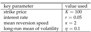
Table 1.Key parameter values for numerical simulations .

key parameter value used

strike price K=100

interest rate r=0.05

mean reversion speed κ=2

long-run mean of volatility η=0.1

market, we proceed withρ=−1 andT=5. For demonstrating the numerical solution and its rate of convergence estimates, we first consider uniform spacial grids. To this end, we may denote that

hm=h, kn =k=σh, m=1, 2, . . . ,M; n=1, 2, . . . ,N.

Results over nonuniform grids will be presented later on. 122

Some key parameters used are shown in Table1. Further, a Crank-Nicolson type temporal 123

integrator will be utilized for advancing our semi-discretized system(2.9),(2.12), with∆τas the 124

temporal step [18]. It has been known thatλ=∆τ/c2, wherec=min{h,k}, play an effective 125

role of the Courant number [14,16]. We experiment with different values ofλvarying from 0.5 to 126

1. 127

Our semi-discretized scheme is expected to be up to the first order in convergence in 128

space. To numerically examine this through experiments, we employ a generalized Milne’s 129

device [13,20]. Then, for a selected terminal timeT, we denote the numerical solution at point 130

(xm,yn,T), 1≤m≤M; 1≤n≤N, asum,n;hfor any particular spatial step 0<h1. Likewise, 131

we letum,n;h/2andum,n;h/4be computed solutions obtained by usingh/2 andh/4, respectively. 132

Thus, the point-wise rate of spatial convergence atTcan be evaluated via 133

Rhm,n ≈

1 ln2ln

u_m,n;h−u_m,n;h/2

u_m,n;h/2−u_m,n;h/4

.

Most of our experiments are accomplished on Apple workstations. Matlab platforms without 134

parallelizations are used throught operations. 135

Let h = 0.01 and σ = 1. For simplicity of notations, we use the same letter v for the 136

approximate solution to(1.1). We show the solutionvforρ=−0.5 andρ=−1 in Figure3and 137

Figure5, respectively. To see more precisely solution profiles, we show corresponding contour 138

maps next to the surfaces. It can be observed that the European put option price is a decreasing 139

function of the stock priceS. This coincides well with the financial theory that a put option price 140

should have a negative correlation with the underline stock price [1,11]. To examine further the 141

delicate relationship between a put option price and its volatility, we plot an average numerical 142

solution ¯v(y,t)taken across different stock prices with respect to the volatility in Figure7. The 143

simulated computational result is exactly what we would expect, since a put option price should 144

Table 2.Rates of convergenceRh_PWobserved withσ=1,ρ=−0.5 andT=0.5.

mesh steps rconv. rates λ=0.5 λ=0.75 λ=1

min

m,n(R

h

m,n) 0.6193 0.6134 0.6026

h=0.01 max

m,n(R

h

m,n) 1.0024 0.9976 0.9811

meanm,n(Rhm,n) 0.9026 0.90438 0.9053 min

m,n(R

h

m,n) 0.6324 0.6221 0.6206

h=0.02 max

m,n(R

h

m,n) 0.9674 1.0007 1.0151

meanm,n(Rhm,n) 0.8342 0.8300 0.8296 min

m,n(R

h

m,n) 0.5824 0.5971 0.6179

h=0.03 max

m,n(R

h

m,n) 0.9941 0.9437 0.9586

meanm,n(Rhm,n) 0.7952 0.8015 0.8142

Figure 3. LEFT: Price of an European put option at T = 0.5 and for ρ = −0.5; RIGHT:

Corresponding contour map

To exam actual performances of our dynamically balanced algorithms, we plot computed 146

rate of convergence surfaces for cases whenρ = −0.5 andρ = −1 in Figure4and Figure6, 147

respectively. In addition, a summary of point-wise convergence rates for the circumstance as 148

ρ = −0.5, T = 0.5 on different spacial grids is given in Table 2. Minor disturbances can be 149

observed in regions where the solution changes fast, in particularly in extreme situations with 150

0.7

0.9 0.8

Rate of Convergence

0.9

250

y

1

0.5

S

150 50

0.1 50 100 150 200 250

S

0.1 0.3 0.5 0.7 0.9

y

Figure 4. LEFT: Point-wise rate of convergence estimate atT=0.5 and forρ=−0.5; RIGHT:

Corresponding contour map

Figure 5.LEFT: Price of an European put option atT=5 and forρ=−1; RIGHT: Corresponding

contour map

-4

0.9 -2

0

y

0.5

Rate of Convergence

250 2

S

150 4

0.1 50 50 100 150 200 250

S 0.1

0.3 0.5 0.7 0.9

y

Figure 6. LEFT: Point-wise rate of convergence estimate atT = 5 and forρ = −1. RIGHT:

0 0.2 0.4 0.6 0.8 1 38

38.5 39

Figure 7.Relation between average price of an European put option with volatility atT=0.5 and forρ=−0.5.

0 50 100 150 200 280

S

0 0.2 0.4 0.6 0.8 1

z 1

0 0.2 0.4 0.6 0.8 1 y

0 0.2 0.4 0.6 0.8 1

z2

Figure 8.LEFT: Nonlinear mesh distribution governing functionz1in theS-direction; RIGHT: Nonlinear mesh distribution governing functionz2in they-direction

0 1 0.2

0.8 ₂₈₀

0.4

Composite Surface

0.6 0.6

y

200

S

0.4 150

0.8

100

0.2 ₅₀

0 0 0 50 100 _S150 200 280

0 0.2 0.4 0.6 0.8 1

y

Now, we consider simulations over nonuniform spacial grids. To better design our tests, we 152

are particularly interested in the following nonlinear distribution governing functions 153

z1(S) =

s

1 2.56+

25(S/100)10

2.56[1+ (S/100)5_]4, Smin≤S≤Smax, z2(y) =

10p

0.5y

7 , ymin≤y≤ymax,

since they asymptotically fit into profiles of our option solutionv as shown in experiments associated with uniform spacial meshes. Our nonuniform grids are generated via an arc-length equal-distribution principal for functionsz1,z2inS- andy-directions, respectively. The principal is commonly utilized in adaptive computations and serves as an initial exploration for more sophisticated adaptations [3,20]. The calculation of the mesh coordinates in our experiments is conducted based on a forward Euler formula for arc-lengths [18]. For instance, in theS-direction we have

Sj+1=Sj+

`

(N−1)q1+ [(z1(Sj))S]2

, j=1, 2, . . .N−1,

where`is the total arc-length, that is,

`= Z S_max

Smin

q

1+ [(z1(S))S]2dS.

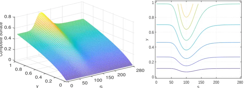
While the distribution functionsz1,z2are shown in Figure8, their composite surface plots can 154

be found in Figure9. The latter characterizes the 2-dimensional profile of our grids distribution. 155

The numerical solution acquired over such nonuniform grids, withρ=−0.5 atT=0.5 is given 156

in Figure??. 157

3. Discussion 158

A dynamically balanced up-downwind semi-discretized finite difference method is 159

constructed and analyzed in this paper based on arbitrary spacial grids. The algorithm acquired 160

is easy to use. It is also effective for solving underlying Heston stochastic volatility option pricing 161

model problems with cross-derivative terms. The scheme is proven to be numerically stable. The 162

numerical method is expected to be first order in space. Computational experiments are carried 163

out to verify our expectations both on uniform and nonuniform grids. 164

The spectral norm is used throughout this paper. The study can be extended by using 165

different Euclidean norms. Our ongoing research has been including effective schemes on 166

variable spacial and temporal meshes for different financial products and simulations. We have 167

also been considering effective adaptation strategies such as those investigated in [16,18]. 168

Our future endeavors also include improving the computational efficiency through 169

exponential splitting methods, particularly variable step LOD approximations [3,8,20]. Compact 170

handling cross-derivatives dynamically and well balances for pricing American and some Asian 172

options [1,7,12,22]. 173

Author Contributions: Conceptualization, C.S. and Q.S.; Methodology, C.S. and Q.S.; Software, C.S.; 174

Validation, C.S. and Q.S.; Formal Analysis, C.S. and Q.S.; Investigation, C.S. and Q.S.; Resources, C.S. and 175

Q.S.;Writing—Original Draft Preparation, C.S.; Writing—Review & Editing, C.S. and Q.S.; Visualization, C.S. 176

and Q.S.; Supervision, Q.S.; Project Administration, C.S. and Q.S.; Funding Acquisition, Q.S. 177

Funding: This research work is partially supported by American Mathematical Society (Fan Research 178

Award: AMS-F-32180177). 179

Acknowledgments:We are grateful to colleagues for their valuable and helpful discussions. 180

Conflicts of Interest:The authors declare no conflict of interest. 181

References 182

1. Albrecher H.; Predota M. On Asian option pricing for NIG Lévy processes.J. Comp. Appl. Math.2004, 183

172,153–168. 184

2. Black F.; Scholes M. The pricing of options and corporate liabilities.J. Political. Econ.1973,81, 637–654. 185

3. Cheng, H.; Lin P.; Sheng Q.; Tan R. Solving degenerate reaction-diffusion equations via variable step 186

Peaceman-Rachford splitting.SIAM J. Sci. Comput.,2003,25, 1273–1292. 187

4. Düring B.; Fournié M. High-order compact finite difference scheme for option pricing in stochastic 188

volatility models.J. Comput. Appl. Math.2012,236, 4462–4473. 189

5. Düring B.; Fournié M.; Heuer C. High-order compact finite difference schemes for option pricing in 190

stochastic volatility models on non-uniform grids.J. Comput. Appl. Math.2014,271, 247–266. 191

6. Fornberg B. Calculation of weights in finite difference formulas.SIAM Rev.1998,40, 685–691. 192

7. Fusai G.; Meucci A. Pricing discretely monitored Asian options under Lévy processes. J. Banking

193

Finance.2008,32, 2076–2088.

194

8. Hendricks C.; Ehrhardt M.; Günther M. High-order ADI schemes for diffusion equations with mixed 195

derivatives in the combination technique.Appl. Numer. Math.2016,101, 36–52. 196

9. Heston S. A Closed-form for options with stochastic volatility with applications to bond and currency 197

options.Rev. Finan. Stud.1993,6, 327–343. 198

10. K. J. in’ t Hout; Welfert B. D. Stability of ADI schemes applied to convection-diffusion equations with 199

mixed derivative terms.Appl. Numer. Math.2007,57, 19–36. 200

11. Hull J. C.Option, futures and other derivatives, 9th ed.; Pearson Education: New Jersey, USA, 2015. 201

12. Ikonen S.; Toivanen J. Efficient numerical methods for pricing American options under stochastic 202

volatility.Numer. Meth. PDEs.2008,24, 104–126. 203

13. Iserles A.A First Course in the Numerical Analysis of Differential Equations, 2nd ed.; Cambridge University 204

Press: New York, USA, 2008. 205

14. Lax P. D.; Richtmyer R. D. Survey of the stability of linear finite difference equations.Comm. Pure Appl.

206

Math.1956,9, 267–293.

207

15. Ma K.; Forsyth P. A. An unconditionally monotone numerical scheme for the two-factor uncertain 208

volatility model.IMA J. Numer. Anal.2017,37, 905–944. 209

16. Meng Q. J.; Ding D.; Sheng Q. Preconditioned iterative methods for fractional diffusion models in 210

finance,Numer. Meth. PDEs.2015,31, 1382–1395. 211

18. Padgett J.; Sheng Q. Numerical solution of degenerate stochastic Kawarada equations via a 213

semi-discretized approach.Appl. Math. Comp.2018,325, 210–226. 214

19. Rachev S. T.Handbook of Computational and Numerical Methods in Finance; Birkhäuser: Boston, USA, 215

2014. 216

20. Sheng Q.; Padgett J. On the stability of a variable step exponential splitting method for solving 217

multidimensional quenching-combustion equations.Springer Proc. Math. Stat.2016,171, 155–167. 218

21. Shreve S.Stochastic Calculus for Finance II: Continuous-Time Models; Springer: New York, USA, 2004. 219

22. Zhu S. P.; Chen W. T. A predictor-corrector scheme based ADI method for pricing American puts with 220