Evolution of heavy quark distribution
function on quark-gluon plasma: Using
the Iterative Laplace Transform Method
Sharareh Mehrabi Pari1,2∗, Kurosh Javidan1∗∗, Fatemeh Taghavi Shahri1∗ ∗ ∗
1 Department of Physics, Ferdowsi University of Mashhad, 91775-1436
Mashhad, Iran
2 Department of Physics and Technology, University of Bergen, 5007
Bergen, Norway
Abstract
The “Iterative Laplace Transform Method” is used to solve the Fokker-Plank equation for finding the time evolution of the heavy quarks distribution functions such as charm and bottom in quark gluon plasma. These solutions will lead us to calculation of nuclear sup-pression factorRAA. The results have good agreement with available experiment data from the PHENIX collaboration.
1
Introduction
Heavy partons, which are produced in the early stage of heavy ion collisions could induce a large amount of energy loss for hard patrons produced in the initial stage of the collision. So, the observed jet quenching in such collisions can indicate the formation of this strongly interacting dense matter [1, 2]. Charm and bottom quarks play crucial role in this endeavor because they are
∗Email: [email protected] ∗∗Email: [email protected]
the witness to the entire space-time evolution of the system and due to their large masses, a memory of their interaction history may be preserved [3].
The Fokker-Plank equation (FPE) provides an appropriate framework for studying the evolution of the heavy quark distribution functions [4].
Heavy quarks dissipate their energy during their propagation through QGP via two processes [5]: The first one is the collisional process and the second one is the radiative process [6].These processes can be described well by the Fokker-Plank equation. In this paper our main task is to study the evolution of heavy quarks in quark gluon plasma by solving the Fokker-Plank equation with a new method named ”Iterative Laplace Transform Method” [7]. This method gives numerical solutions in the form of conver-gent series. To verify our solutions, we calculate the nuclear suppression factor, RAA(pT), of heavy quarks using simulated data of heavy ion colli-sions [8].To do this we consider both the collisional and radiation parts of energy loss in FPE and finally we compare our results with experimental data from PHENIX [9].
2
The heavy quark momentum evolution in FPE
dynamics
The Quark Gluon Plasma (QGP) is formed at the timeτi after the impact. Time evolution of the momentum distribution of non-equilibrated heavy quarks due to the interaction with the equilibrated QGP during the time interval τi < τ < τHQ can be calculated by the Fokker-Plank equation as follow:
∂f(p, t)
∂t =A(p) ∂
∂p(pf(p, t)) +D(p)
∂ ∂p
2
f(p, t) . (1)
Where A is drag and D is diffussion coefficients.The drag coefficient is an important quantity carrying information about the dynamics of elastic col-lisions. It is expected that the drag coefficient should be determined by the properties of the bath and not by the nature of the HQ. In this work we use the drag coefficient as follows:
A(p, t) =−1
p dE
dL . (2)
considering ”Hard and Soft Thermal Loops” are given as follows [11]. For
E MT2:
−dE
dL =
8πα2sT2
3
1 +nf 6
1
v −
1−v2
2v2 ln(
1 +v
1−v)
ln
2
nf
6+nfB(v) ET
mgM
,
(3) forE MT2:
−dE
dL =
8πα2sT2
3
1 +nf 6 ln 2 1
2(6+nfnf)0.92
√
ET mg
, (4)
where v is the HQ speed, αs is the strong coupling constant, nf is the number of quark flavors in the medium, E and M are energy and mass of the propagated HQ respectively, mg =
(1 +nf/6)g2T2/3 is the thermal gluon mass, g = √4παs is the gauge coupling parameter and B(v) is a smooth velocity function, which can be taken approximately as 0.7 [11]. Finally the total energy loss due to both collision and radiation precesses is:
−dEtotal
dL =
10α2sT2
3 ln
3E
8παsT
ln
ξ+1 +ξ2
+ξln 1 ξ+ 1 + 1
ξ2 + 3 8π (5) where ξ = 29πE3T. Using equation (4),(5), we will calculate the drag and diffusion coefficients for HQ energy loss during the interaction with QGP medium. In the next section we will find the solution of the Fokker-plank equation, eq(1).
3
The Iterative Laplace Transform Method
In this section we want to introduce a new method for solving the FP equation, namely the ”Iterative Laplace Transform Method” (ILTM) [7]. This new method was proposed by Daftardar-Gejji and Jafari to seek nu-merical solutions of nonlinear functional equations. This method is called the Iterative Laplace Transform Method, which is a combination of two powerful methods, namely, the Laplace transform method and the Iterative method. The method gives numerical solutions in the form of convergent series with easily computable components. The most outstanding feature of this method is that it provides an analytical solution using the initial condi-tions only, without any discretization or restrictive assumpcondi-tions. In general, the Fokker-Plank equation can be written as [7]:
Dαtf =
DβpA(p, t, f) +D2pβB(p, t, f)
Here Dαt(.), Dβp(.), Dp2β(.) are the Caputo fractional derivative with respect totand p.
In our calculations we use the following definitions:
I. The Caputo fractional derivative of function (p, t) is defined as
Dtαf(p, t) = 1 Γ(m−α)
(t−η)m−α−1fm(p, η)dη (7) form−1< α≤m,m∈N.
II. Laplace transform of Dtαf(p, t) is given by
L[Dtαf(p, t)] =xαL[f(p, t)]− m−1
k=0
f(k)(p,0)xα−1−k; m−1< α≤m , (8)
wheref(k)(p,0) is the kth derivative of f(p, t) at t= 0.
To illustrate how the iterative Laplace transform method works, the general space-time fractional partial differential equation is considered
Dtαf =A(f, Dβpf, Dp2βf, ...) m−1 < α≤m
n−1< β≤n m, n∈N , (9)
where A(f, Dpβf, D2pβf, ...) is a linear or nonlinear operator of
f, Dβpf, Dp2βf, ....
With the initial condition
f(k)(p,0) =hk(p); k= 0,1, ..., m−1, (10) and f(p, t) will be determined later.
First of all we take the Laplace transform of both sides of (9)
xαL[f(p, t)]− m−1
k=0
xα−1−kf(k)(p,0) =L[A(f, Dβpf, Dp2βf, ...)]. (11)
After simplification, we have
L[f(p, t)] = m−1
k=0
x−1−kf(k)(p,0) +x−αL[A(f, Dβpf, D2pβf, ...)]. (12)
f(p, t) =L−1[ m−1
k=0
x−1−kf(k)(p,0)] +L−1[x−αL[A(f, Dβpf, Dp2βf, ...)]],
(13) Then we set
f0 =L−1 m−1
k=0
x−1−kf(k)(p,0)
,
f1 =L−1[x−αL[A(f, Dβpf, Dp2βf, ...)]]
If we want to calculate the next term in the series we have to considerf1 as initial condition and putting it in the equation (9) and repeat all the above steps. Therefore the solution of (9) with initial condition (10) is given by:
f(p, t)∼=f0(p, t) +f1(p, t) +...+fm(p, t), m= 1,2, ... (14) If we set α = β = 1 in Equation (9) we will reach the FPE. We solved the FPE using both finite difference method and ILTM with different types of initial conditions and compared their results. For initial conditions with non vanishing values at the borderer, the ILTM successfully solves the FPE while results of finite difference method diverges and therefore it failes to find the solution. We have taken transverse momentum distribution functions of charm and bottom quarks at√s= 200GeV in Au-Au and also P-P collisions from [12]. ILTM has been performed up to m= 2.
4
Calculating
the
nuclear
suppression
factor
R
AA(
P
T)
The dissipation coefficients of the thermal bath and initial momentum distri-bution of HQs, are basic inputs required to solve the FPE. In our calculation the time dependence of temperature is taken from [13]. Here we considered a fixed value for coupling constant asαs = 0.3.
Figure 1 demonstrates the drag coefficient for b and c quarks due to collision and radiation separately. This figure clearly shows that the energy loss forc quark is greater than that forbquark.
Figure 1: The drag coefficient due to collision and radiation as functions of momentum for Bottom and Charm quarks in QGP.
or non-photonic single e− spectra resulting from semi leptonic decays of hadrons containing charm and bottom quarks) produced in Nucleus-Nucleus collisions with respect to those produced in proton-proton collisions which is formulated in nuclear suppression factor RAA.
Here the nuclear modification factor in relativistic heavy ion collisions is calculated for demonstrating the power of ILTM applied to solve the FP equation. The solution of the FP equation have been convoluted with the fragmentation functions of the heavy quarks to obtain thePT distribution of the heavy mesons [13]. Similar simulations also have been performed to find
Figure 2: Nuclear suppression factor RAA due to collisional and radiation energy loss separately as functions of PT. Used parameters are: τ0 = 0.33 fm/c, T0 = 0.375 GeV,
αs= 0.3, Tc= 0.175 GeV [13].
distribution functions of proton at√s= 200GeV have been taken as initial conditions to solve FPE again. The ratio of these two quantities is propor-tional to the nuclear suppression factor,RAA measured in experiments:
RAA(PT)∝ dNe dPTdη
Au−Au
dNe dPTdη
P−P (15)
A small value of RAA indicates a strong suppression and therefore, large energy loss of heavy quarks in the medium. It is clear that this ratio is equal to one in the absence of any medium.
Figure 2 presents contribution of collision and radiation energy loss in suppression factor RAA separately. Displayed experimental data has been obtained from the PHENIX collaborations forAu+Aucollisions at√sN N = 200GeV. This figure shows that suppression at higher values ofPT can not be explained by collisional energy loss. In other words, contribution of radiation in energy loss at higher PT is more important than collisional energy loss only.
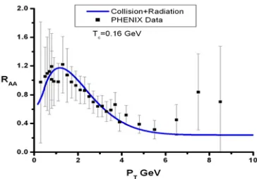
Figure 3: Nuclear suppression factorRAAas function ofPT. Energy loss due to collision and radiation have been considered in calculating the drag coefficient.
5
Conclusions and remarks
we calculated the nuclear suppression factor RAA. It is shown that there is a good agreement between simulation results and reported experimental data (fig. 3).
References
[1] W. Scheid, M. Muller and W. Greiner, PRL 32, 741 (1974). G. F. Chapline, M. H. Johnsou, E. Teller, M. S. Weiss PRD8, 135 (1973). L. P. Csernai, et al., PRC25, 2482 (1982).
[2] J.Y. Ollitrault, Eur. J. Phys. 29, 275 (2008 ).
[3] B. Svetitsky Phys. Rev. D 37, 2484 (1988).
[4] M. L. Mangano, P. Nason and G. Ridolfi, Nucl. Phys. B 538, 282 (2002).
[5] S. Mazumder, T. Bhattacharyya, J. Alam and S.K. Das, Phys. Rev. C 84, 044901 (2011).
[6] B. Z. Kopeliovich, I. K. Potashnikova, I. Schmidt, Phy. Rev. C 82, 037901 (2010).
[7] L. Yan, Hindawi Publishing Corporation, Volume 2013, Article ID 465160.
[8] S.K. Das, F. Scardina, S. Plumari, and V. Greco, Phys. Rev. C 90, 044901 (2014).
[9] S. S. Adler et al., (PHENIX Collaboration), Phys. Rev. C 84, 044905 (2011).
[10] A.K. Chaudhuri, V.P. Goncalves, and L. F. Mackedanz, Brazilian Jour-nal of Physics, 37,no 2B (2007).
[11] M. B. Gay Ducati, V. P. Goncalves and L. F. Mackedanz, Brazilian Journal of Physics, 37, 656-660 (2007).
[12] M. Cacciari, P. Nason, R. Vogt, PRL 95, 122001 (2005)