University of South Carolina
Scholar Commons
Theses and Dissertations
5-2017
Advances in Chemistry, Part I: Noise, Calibration,
and Educational Advances In Analytical Chemistry.
Part II: Safety Oversight in Chemical Journals
Lauren E. Grabowski
University of South Carolina
Follow this and additional works at:https://scholarcommons.sc.edu/etd
Part of theArts and Humanities Commons, and theChemistry Commons
This Open Access Dissertation is brought to you by Scholar Commons. It has been accepted for inclusion in Theses and Dissertations by an authorized administrator of Scholar Commons. For more information, please [email protected].
Recommended Citation
ADVANCES IN CHEMISTRY.PART I:NOISE,CALIBRATION, AND EDUCATIONAL ADVANCES IN ANALYTICAL CHEMISTRY.PART II:SAFETY OVERSIGHT IN CHEMICAL JOURNALS.
by
Lauren E. Grabowski Bachelor of Science Saint Francis University, 2012
Submitted in Partial Fulfillment of the Requirements For the Degree of Doctor of Philosophy in
Chemistry
College of Arts and Sciences University of South Carolina
2017 Accepted by:
Scott R. Goode, Major Professor Stephen L. Morgan, Committee Member
Caryn E. Outten, Committee Member Matthew Miller, Committee Member
ii
iii DEDICATION
To My Parents
iv
ACKNOWLEDGEMENTS
Thank you to everyone I have ever met. Whether you know it or not, you helped shape my aspirations.
I would like to thank my committee members Dr. Morgan, Dr. Outten, and
Dr. Miller. Thanks to my undergraduate advisor, Dr Balazs Hargittai, who
encouraged me to attend graduate school. I also would like to thank Alice
Flarend and Gene Yingling, my high school science teachers, whose enjoyable
classes solidified my love of science.
The love and support of my family has allowed me to accomplish all that I have today. To Cassie for always believing in me, even though I didn’t always believe in myself. I am forever grateful.
v ABSTRACT
Part I
The accuracy and precision of the results of any chemical analysis depends on the calibration graph and its associated systematic and random errors. Least squares regression generally treats all data with equal weights. A weighted least-squares fit is an improvement but requires knowledge of the imprecision in each point of the calibration graph. The imprecision is not easy to estimate with high confidence because of the large number of replicates needed.
The imprecision depends on the types and magnitudes of the sources of noise. We characterized the noise sources in ICP-OES and UV/Vis and
developed a model that effectively predicts the standard deviation of emission and absorption as a function of concentration.
Once a model is fit to the data, calibration designs were studied. These designs ranged from one to three decades of response and concentration in order to optimize precision over the entire calibration space for ultraviolet-visible spectrochemical analyses. Different calibration strategies, composed of different concentrations and numbers of replicates, have been evaluated determine the calibration design that minimizes imprecision as measured by the average relative concentration error integrated over the entire calibration graph.
vi
titrations. Students performed a potentiometric titration to determine the initial analyte concentration and reactant concentrations at varying points in the titration in order to determine the solubility product constant of a solid species.
Part II
Advances in chemistry are highly dependent on the procedures published in peer-reviewed journals. Some chemistry journals require authors to address safety considerations in their manuscripts but others do not. In this study, we examined 726 chemistry journals from 28 publishers to determine if they require the author to mention safety precautions. Journals supply information for authors that generally mention safety in two places. In the guidelines for authors, which are widely read by prospective contributors, 8% mention safety. Most journals have ethics guidelines of which 59% mention safety.
In order to determine the effectiveness of safety policies 100 articles from each of six journals that published research that involved extensive syntheses were selected. The results of the search indicated that the target compounds were mentioned 107 times but only one mention carried any safety precaution.
vii
TABLE OF CONTENTS
DEDICATION ... iii
ACKNOWLEDGEMENTS ... iv
ABSTRACT ... v
LIST OF TABLES ... viii
LIST OF FIGURES ... ix
LIST OF ABBREVIATIONS ... xi
CHAPTER 1:NOISE SOURCE CHARACTERIZATION OF INDUCTIVELY COUPLED PLASMA –OPTICAL EMISSION SPECTROSCOPY ... 1
CHAPTER 2:EXPERIMENTAL VALIDATION OF UNCERTAINTY RELATIONSHIPS IN CALIBRATIONS FOR ULTRAVIOLET/VISIBLE ABSORPTION SPECTROSCOPY ... 18
CHAPTER 3:DETERMINING A SOLUBILITY PRODUCT CONSTANT BY POTENTIOMETRIC TITRATION TO INCREASE STUDENTS’CONCEPTUAL UNDERSTANDING OF POTENTIOMETRY AND TITRATIONS... 40
CHAPTER 4:REVIEW AND ANALYSIS OF SAFETY POLICIES OF CHEMICAL JOURNALS ... 53
CHAPTER 5:RESPONSE TO REVIEW AND ANALYSIS OF SAFETY POLICIES OF CHEMICAL JOURNALS ... 77
APPENDIX A–CHAPTER 3SUPPORTING INFORMATION ... 85
viii
LIST OF TABLES
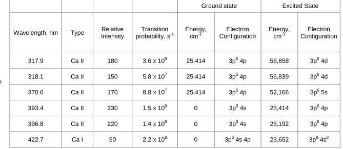
Table 1.1 Calcium Wavelengths and Transitions. ... 9
Table 1.2 Values of β at Ca Wavelengths ... 10
Table 2.1 Signal to Noise Ratio of Different Decades, 348.0 nm, NMC ... 30
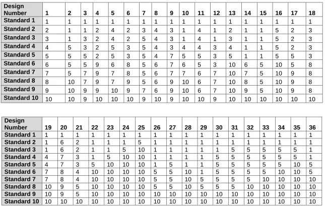
Table 2.2 Calibration Designs, Relative Concentration of each of the ten standards ... 31
Table 2.3 Best 3 Calibration Designs for Each Decade, 348.0 nm, NMC ... 32
Table 3.1 Calculated Ksp Values Taken for Three Points After the Equivalence Point ... 50
Table 4.1 Appearance of Safety Keywords in Journal Guidelines for Authors ... 69
Table 4.2 Frequency of Reading Ethics Guidelines ... 70
Table 4.3 Perceptions of Contents of Ethics Guidelines ... 71
Table 4.4 Number of Journal Articles Containing a Safety Keyword ... 72
Table 4.5 The Number of Articles that Mentioned the Target Compounds ... 73
Table 4.6 Locations in Which Safety Should be Mentioned Specific by Guidelines for Authors ... 74
Table 4.7 The Use of Safety Keyword ... 75
ix
LIST OF FIGURES
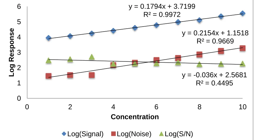
Figure 1.1 Experimental Measurements of Ca Emission at 393.4nm ... 11
Figure 1.2 Calcium Signal-to-Noise Ratio at 317.9 nm , 0.1-400 ppm ... 12
Figure 1.3 Calcium Signal-to-Noise Ratio at 318.1 nm, 3.13-1000 ppm ... 13
Figure 1.4 Calcium Signal-to-Noise Ratio at 370.6 nm, 5.00-1000 ppm ... 14
Figure 1.5 Calcium Signal-to-Noise Ratio at 393.4 nm, 0.05-6.25 ppm ... 15
Figure 1.6 Calcium Signal-to-Noise Ratio at 396.8 nm, 0.05-6.25 ppm ... 16
Figure 1.7 Calcium Signal-to-Noise Ratio at 422.7 nm, 0.1-400 ppm ... 17
Figure 2.1Calibration Concentration Error of all designs, 3-decade concentration range, 348.0 nm, NMC ... 33
Figure 2.2 CCE Comparison of the UV region (348 nm) to the visible region (435 nm), 3-decade concentration range, MC, standard deviations not shown ... 34
Figure 2.3 Absorption Spectrum of Potassium Dichromate ... 35
Figure 2.4 Comparison of MC and NMC relative to the CCE of each design, 3-decade, 435.0 nm... 36
Figure 2.5 Comparison of single-decade designs: 0.002-0.02 AU, 0.02-0.2 AU, and 0.2-2.0AU, without standard deviations, 348.0 nm, NMC ... 37
Figure 2.6 Two-Decade Concentration without standard deviations, 435.0 nm, MC.. ... 38
Figure 2.6 Calibration Concentration Error Comparison for all designs, 348.0 nm, NMC... ... 39
x
Figure 3.2 Experimental data. A) Titration curve B) Derivative
(difference between successive points). ... 52
Figure 4.1 Distribution of safety keywords in journal ethics guidelines ... 76
Figure A.1 Titration set up with electrodes ... 87
Figure A.2 BNC-T connection to the LabQuest unit ... 87
xi
LIST OF ABBREVIATIONS
ACS ... American Chemical Society AU ... Absorbance Units C&EN ... Chemical and Engineering News CAS ... Chemical Abstract Service CCE ... Calibration Concentration Error CCS ... Committee on Chemical Safety CHAS ... Division of Chemical Health and Safety CHED ... Division of Chemical Education GAANN ... Graduate Assistance in Areas of National Need ICP-OES ... Inductively Coupled Plasma – Optical Emission Spectroscopy JACS ... Journal of the American Chemical Society Ka ... weak acid ionization constant
Ksp ... solubility product constant
pKsp ... logarithmic value of the solubility product constant
1
CHAPTER
1
NOISE SOURCE CHARACTERIZATION OF INDUCTIVELY
COUPLED PLASMA - OPTICAL EMISSION SPECTROPSCOPY
1.1 ABSTRACT
The accuracy and precision of the results of any chemical analysis depends on the calibration graph and its associated systematic and random errors.
Calibration graphs are, in theory, simple: results (emission intensities in the case of the ICP-OES instrument) are graphed as a function of concentration and an appropriate model is fit to the data by least squares regression. But this process generally treats all data with equal weights.
A weighted least-squares fit is an improvement but requires knowledge of the imprecision in each point of the calibration graph. The imprecision is not easy to estimate with high confidence because of the large number of replicates
needed.
2
1.2 INTRODUCTION
Inductively Coupled Plasma – Optical Emission Spectroscopy (ICP-OES) has risen to be a widely-used emission technique for determining the elemental composition of aqueous samples.1 The principal advantages of ICP-OES is its wide linear dynamic range of 108 and relative freedom from inter-element interferences.2
A major advancement in ICP-OES was the introduction of a charge injection device (CID) detector. A CID detector allows for quick measurement of high intensity signals but longer measurement of low intensity signals for
protection from saturation and optimal signal to noise.3 Blooming is also minimized compared to the more common charge coupled device (CCD) detector.
Multi-wavelength array detectors changed the course of measurements made with ICP-OES. ICP-OES is now a reliable, low cost, exceedingly efficient instrument for high-precision analysis.
This study was aimed at enhancing high-precision analysis by modeling the standard deviation. A detailed study of the heteroscedastic noise was analyzed to determine proper weights for the incorporation of weighted least-squares regression analysis.
1.3 NOISE SOURCES
3
we will define “noise” as the imprecision as measured by the standard deviation of a measurement. If the noise in the experiment is constant and independent of the concentration (or response) then Gaussian statistics can be used. However, precision in measurements in a real laboratory setting depend upon the
response, thus non-uniform precision (heteroscedasticity) is found.
Understanding heteroscedasticity requires a detailed study of noise sources. There are a number of ways to classify noise sources but one of the most useful is based on the mathematical dependence of the noise to the response.4,5
Independent of Response Noise sources independent of the response include thermal detector noise. This electronic noise occurs inside the electrical
conductor as electrons are thermally agitated, which happens regardless of any applied voltage.6 Thermal noise is always present in a measurement and only disappears at absolute zero. The noise in components like resister (Johnson noise) is similar.
4
integration time, which allows for more photons and charge to accumulate on the charge injection device detector.
Directly Proportional to the Response Noise proportional to the response includes flicker noise that tracks fluctuations in source intensity and slight
wavelength shifts along the detector axis.7 Noise proportional to the response is the limiting noise factor at high concentration.8
1.4 DEPENDENCE ON SIGNAL
Since the noise is heavily dependent on the response, a three parameter fit (the parameters are the magnitudes of the noise independent of the concentration, noise related to the square root of concentration, and noise related to the
concentration) was fit to allow estimation of noise at intermediate concentrations. The noise was modeled by the equation: I 1 2 I 3I where β1, β2, and
β3 are constants for the instrument at a specific wavelength.4 At smaller
intensities, β1 is the dominant noise source, whereas at higher intensities, β2 and
β3 dominate.9 Since ICP-OES is linear over a wide dynamic range, the limiting
noise strongly depends on the analyte concentration.
1.5 EXPERIMENTAL MEASUREMENT OF SIGNAL TO NOISE RATIO
5
All analyte solutions were prepared by diluting a calcium stock solution (1000 ppm Ca in 2% hydrochloric acid) with 2% HCl. Analyte concentrations were chosen to match the linear intensity range for each wavelength, discussed in the next section. Each aliquot was weighed such that the calculated
concentrations of the standards were free from pipetting imprecision.
1.6 CHOICE OF WAVELENGTH
Calcium has a number of suggested analytical wavelengths with relative intensities of 40,000 to 70,000,000. These numbers indicate the signal
magnitude per unit calcium concentration. Typically, low sensitivity wavelengths are chosen when the calcium concentrations in the sample are relatively high. The emission at the less-sensitive wavelengths will not saturate the detector so the sample can be analyzed without dilution. The more sensitive wavelengths afford the analysis of ultratrace (sub-mg/L, or sub-ppm) concentrations. These lines provide better limits of detection - the detection limit for calcium in the ICP is 0.05 ppm – and allow the experimenter to dilute the sample to minimize matrix effects.
The varying intensities or sensitivities arise from fundamental sources such as the ICP temperature and the excitation processes. The spectrum includes emission from neutral atoms as well as from ions and transitions that terminate in the ground state, others do not. And the population of the excited state is dependent on the plasma condition such as temperature and the energy level of the excited state.
6
different concentrations of Ca standard were obtained. Concentrations varied from 0.05-1,000 ppm depending on the intensity of calcium at each wavelength. The concentrations were all evenly spaced when converted to the log-log scale. The fundamental characteristics of the lines are shown in Table 1.1. Ca I is traditional spectroscopic notation that indicates a neutral line and Ca II is the first ion line (emission from Ca+). The relative intensities from the NIST database are included for completeness, but they are generated from a different emission system (a wall-stabilized arc) than the ICP.
1.7 RESULTS AND DISCUSSION
One hundred integrations of each solution were recorded and the signal and noise were calculated, as depicted in Figure 1.1. It can be noted that as the log of the signal increases, the log of the noise also increases. Though, the signal-to-noise ratio is fairly constant, thus flicker signal-to-noise is the limiting signal-to-noise source.
The values of β1, β2, and β3 for calcium wavelengths are shown in Table
1.2. The constant, β, with the highest value identifies the limiting noise. At 393.4 nm, β1 = -7.0965, β2 = -0.2922, and β3 = 16.1294. In this case, the larger value of
β3 is consistent with the limiting noise being flicker noise. At lower intensity
wavelengths, such as 422.7nm, β1 is the limiting noise source. These findings
are consistent with previous research.9
7
The models are good representation of the predicted noise. In some cases, the experimental measurement such as the first point at 317.9nm skews the model since the concentration is relatively close to the detection limit. This issue could be eliminated by making measurements much greater than the limit of detection but the purpose of this study was to examine the largest possible linear dynamic range.
The two wavelengths with the highest relative intensities, 393.4 and 396.8 nm, are flicker noise limited at the three highest concentrations. The other four wavelengths show an initial increase in signal to noise ratio consistent with that of detector noise.
1.8 CONCLUSION
The model fits the data remarkably well, considering that we are modeling the uncertainty in the emission signal as a function of the concentration.
The application of this work is to improve the accuracy and precision of multi-decade calibration curves by using weighted least squares fits. Because the noise sources are heteroscedastic the magnitude of the noise depends on the emission signal; and this work provides informed estimates of the
relationships that can be used to predict weights with some amount of confidence.
1.9 ACKNOWLEDGEMENTS
8
1.10 REFERENCES
1. Fassel, V. A.; Kniseley, R.N., Anal. Chem. 1974, 46, 1017-1021. 2. Watters, R. L.; Carroll, R. J.; Spiegelman, C. H., Anal. Chem. 1987, 59,
1639-1643.
3. Thermo Electron Corporation. iCAP 6000 Series ICP Emission Spectrometer, 2006.
4. Ingle, J.D. Jr.; Crouch, S.R., Spectrochemical Analysis; Prentice Hall: Englewood Cliffs, 1988.
5. Ingle, J. D. Jr.; Crouch, S. R., Anal. Chem. 1972, 44, 1375-1386. 6. Skoog, D. A.; Holler, F. J.; Crouch, S. F., Instrumental Analysis;
Brooks/Cole: Belmont, 2007.
7. Rothman, L. D.; Crouch, S. R.; Ingle, J. D. Jr., Anal. Chem. 1975, 47,
1226-1233.
9
Table 1.1: Calcium Wavelengths and Transitions.10
Ground state Excited State
Wavelength, nm Type Relative Intensity
Transition probability, s-1
Energy, cm-1
Electron Configuration
Energy, cm-1
Electron Configuration
10
Table 1.2: Values of β at Ca Wavelengths Wavelength,
nm
Minimum Concentration, ppm
Maximum Concentration, ppm
Relative
11
Figure 1.1: Experimental Measurements of Ca Emission at 393.4nm y = 0.1794x + 3.7199
R² = 0.9972
y = 0.2154x + 1.1518 R² = 0.9669
y = -0.036x + 2.5681 R² = 0.4495 0
1 2 3 4 5 6
0 2 4 6 8 10
Log
Res
ponse
Concentration
12
Figure 1.2: Calcium Signal-to-Noise Ratio at 317.9 nm, 0.1-400 ppm 0
0.5 1 1.5 2 2.5 3
0 2 4 6 8 10
Log(
S
igna
l
to
Nois
e
Ratio)
Concentration
13
Figure 1.3: Calcium Signal-to-Noise Ratio at 318.1 nm, 3.13-1000 ppm 2.25
2.3 2.35 2.4 2.45 2.5 2.55 2.6 2.65
0 2 4 6 8 10
Log(
S
igna
l
to
Nois
e
Ratio)
Concentration
14
Figure 1.4: Calcium Signal-to-Noise Ratio at 370.6 nm, 5.00-1000 ppm 0
0.5 1 1.5 2 2.5 3 3.5
0 2 4 6 8 10
Log(
S
igna
l
to
Nois
e
Ratio)
Concentration
15
Figure 1.5: Calcium Signal-to-Noise Ratio at 393.4 nm, 0.05-3.125 ppm 0
0.5 1 1.5 2 2.5 3
0 2 4 6 8 10
Log(
S
igna
l
to
Nois
e
Ratio)
Concentration
16
Figure 1.6: Calcium Signal-to-Noise Ratio at 396.8 nm, 0.05-6.25 ppm 0
0.5 1 1.5 2 2.5 3
0 2 4 6 8 10
Log(
S
igna
l
to
Nois
e
Ratio)
Concentration
17
Figure 1.7: Calcium Signal-to-Noise Ratio at 422.7 nm, 0.1-400 ppm 0
0.5 1 1.5 2 2.5 3
0 2 4 6 8 10
Log(
S
igna
l
to
Nois
e
Ratio)
Concentration
18
CHAPTER
2
E
XPERIMENTALV
ALIDATION OFU
NCERTAINTYR
ELATIONSHIP INC
ALIBRATIONS FORU
LTRAVIOLET/V
ISIBLEA
BSORPTIONS
PECTROSCOPY2.1 ABSTRACT
Ultraviolet-visible absorption spectroscopy is a widely-used technique for quantitative analysis. Although there have been many studies examining the relative concentration error associated with ultraviolet-visible measurements, there is little that addresses the use of modern instruments capable of measuring absorbances that vary over three decades with high accuracy and precision. There is no information to help optimize calibration curves to minimize
spectrophotometric imprecision.
The major source of this spectrophotometric imprecision is detector noise, which obscures and degrades the ability to interpret the response and is
dominant at low concentrations. Random instrumental noise in
19
sources affect the signal-to-noise ratio of ultraviolet-visible absorbance
measurements. The goal of this study was to design calibration strategies that optimize precision over the calibration graph for ultraviolet-visible
spectrochemical analyses for one, two, or three decades of concentration. Different calibration strategies, composed of different concentrations and number of replicates, have been evaluated to try to determine the calibration design that will minimize imprecision as measured by the average relative concentration error integrated over the entire calibration graph.
2.2 INTRODUCTION
Calibration Graphs. Calibration graphs are utilized by chemists to determine the relationship between the analyte concentration and response. This research reports the influence of empirically-chosen calibration designs on the analysis precision.
Calibration Concentration Error. Most labs are comfortable with using the relative standard deviation (rsd) as a measure of precision, thus minimizing rsd (
C/C, which is equal to A/A). Like many other researchers, 1-5
we propose to use
the relative concentration error, σc/C, as the metric to be minimized. Early
research6 showed that for absorbance measurements, the relative concentration error for an individual measurement depended on the absorbance or
20
Ingle and Crouch7 noted that the precision was related to the noise sources that were often complex and had to be measured for an individual instrument. Previous work has examined the minimizing the rsd of individual measurements, though none have looked at the effects of noise on the overall calibration graph. If the relative standard deviation of the concentration can be predicted at each point along the calibration graph the relative concentration error can be integrated between the lowest standard and highest standard to determine the Calibration Concentration Error (CCE). Exploring how the CCE changes as a function of the choice of calibration concentrations was the objective of this research.
Transmittance Measurements. All spectrophometric instruments use detectors that response to intensity, so transmittance, rather than absorbance, is used. Since A=log(1/T), where T is the ratio of transmitted to radiant intensity (T=I/I0),
the variance in absorbance can be determined from the variance in
transmittance. Propagation of uncertainty applied to Beer’s Law states that σc/c=
σA/A.8 The absorbance uncertainty is directly related to the standard deviation of
the transmittance measurement; propagation of error treatment yields the equation: 0.434
T log( )
A T
A T
Noise. Every analytical measurement is made up of two components, the first is the response that contains the information desired and the second is noise. Noise obscures and degrades the ability to interpret the response. For our
21
independent of the concentration (or response), then Gaussian statistics can be used to show the calibration graph with just two points at the extremes of
concentration minimizes the imprecision.9
However, precision in measurements in a real laboratory setting is
dependent upon the response. Thus, non-uniform precision (heteroscedasticity) is assumed for a given calibration graph.10 Heteroscedasticity requires a detailed study of noise sources and a numerical investigation of the average relative concentration error. This study focuses solely on the precision of measurements that are restricted by noise associated with the instrument.
There are a number of ways to classify noise sources but one of the most
useful is based on the dependence of the noise source on the signal.
6
Noise sources independent of the signal include detector noise, many electronic sources, and imprecision due to limited resolution of the readout or
analog-to-digital convertor.
7
Electronic noise occurs inside the electrical
22
Noise proportional to the square root of the signal is dominated by quantum noise. One source of quantum noise is caused by the random
movement of electrons or charged particles across boundaries in semi-conductor circuits.6 The magnitude of this variance increases with signal. A second source is the random arrival rate of photons, which follow a Poisson distribution. The variance is equal to the total number of photons collected. Thus, when the accumulated number of photons is small, quantum noise is more apparent.12
Instruments that use low noise amplification and high resolution readout devices have maximum precision in the range of 0-11% T and are quantum noise limited.7 The amplifier also has its own independent noise associated with it due to the use of resistors and op amps; which will amplify any noise already present in the system. To attenuate this noise, a difference amplifier can be employed.13
Noise proportional to signal includes source flicker noise and
sample-cell positioning imprecision.
14
Source flicker noise is due to fluctuation in source intensity. Unfortunately, flicker noise is not well understood, though it is known to be frequency dependent and larger at low frequencies.12 Another source of noise proportional to the signal is cell positioning imprecision. Reflective losses and transparency differences because of cell imperfections result in position dependence.6 Systematic errors via reflective losses have been previously studied.15
2.3 DESIGN OF EXPERIMENT
0.002-23
2
1 2 3
M k k M M k M
2
2 2
int
2 2
(M int) ( )
slope c M C slope
0.02 Absorbance Units (AU), 0.02-0.2 AU, 0.2-2.0 AU, 2 decade: 0.002-0.2 AU, 0.02-2.0 AU and 3 decade: 0.002-2.0 AU. The 2 and 3 decade concentrations were evenly spaced on the log scale. A three
parameter fit (the parameters are the magnitudes of the noise independent of the concentration, noise related to the square root of concentration, and noise related to the concentration) was fit to the data to allow estimation of noise at intermediate concentrations, as depicted in Figure 2.1.
Thirty-six different calibration designs were employed to predict the standard deviation of the measurement at any particular concentration. Three-decimal place measurements were determined by generating random numbers with the appropriate standard deviations. A regression analysis of the calibration graph resulted in the slope, standard deviation of the slope, intercept and
standard deviation of the intercept. Propagation of errors was used to determine the relative concentration errors: This process was equally spaced over the absorbance units range 199 times. The CCE were determined by summing the relative concentration errors over the calibration graph.
24
2.4 INSTRUMENTATION AND METHODS
Spectrophotometer. The instrument used in this study was a dual-beam molecular absorption spectrophotometer (Varian Cary 50) with a Czerny-Turner monochromator, dual Silicon diode detectors, and a full spectrum Xenon flash lamp with a limiting resolution and spectral bandwidth of 1.5 nm.
Reagents. All analyte solutions were prepared by diluting a potassium dichromate stock solution (1000 ppm K
2Cr2O7 in 0.01M sulfuric acid) with 0.01 M
H
2SO4. Analyte solution concentrations were chosen to range from 0.002-2.0 AU.
Each aliquot was weighed such that the calculated concentrations of the calibration standards were based on gravimetric data.
Measurements. One hundred replicates for each concentration were acquired at 348.0 and 435.0 nm. These measurements were made in the ultraviolet (348 nm) and visible (435 nm) regions because their noise sources are likely to differ. At each wavelength, measurements were made for MC, MCBS, and NMC.
Calibration Range. Calibrations over one decade change in absorbance were made for 0.002-0.02, 0.02-0.2, and 0.2-2.0 AU on the linear scale. Calibrations were performed on the log scale for 2, and 3-decade concentration ranges. Two decade comparisons were made between 0.02-2.0 and 0.002-0.2 AU, and the three decade concentration range was 0.002-2.0 AU.
2.5 RESULTS
25
Designs. Thirty-six different designs were tested in which the number of replicates was changed along with calibration placement across one, two, or three decades of concentration. Table 2.2 lists the designs. When the design results are compared, as depicted in Figure 2.1, differences between the designs is small because the standard deviation of the calibration concentration error is high.
Wavelength Comparison. The samples were run in both the ultraviolet (348.0 nm) and visible (435.0 nm) regions, to enable comparison of noise sources in these regions. Upon overlapping the two wavelengths, as shown in Figure 2.2, it is apparent that the calibration graph designs are not wavelength dependent. Thus, these calibration designs are useful for different wavelengths of ultraviolet-visible absorption spectroscopy. It can also been seen that the CCE for 348 nm is much smaller than that of 435 nm, most likely because of the larger absorbance in the UV, as depicted by Figure 2.3.
Cell Positioning Error. Results indicate there is a correlation between higher imprecision and moving the cell between each sample, which agrees with that of
others,
3
shown in Figure 2.4. These results were expected, as reflective and transparency losses at the glass/air and glass/sample interface result in more noise.
One Decade Comparison. Comparison of the three different 1 decade
26
was 0.7 ± 0.1 and 0.2-2.0 AU was 0.4 ± 0.2. This result is to be expected as the average signal to noise ratio of 0.002-0.02 was 112, with the other two being 1403 and 2962 respectively.
Two Decade Comparison. Two different two-decades were examined to
determine whether the concentration of the standards (low 0.002-0.2 AU or high 0.02-2.0 AU) affected the calibration concentration error. Figure 2.6 depicts the differences between the two-decade concentrations.
The differences between the two-decades at different concentrations is apparent. At lower concentrations, 0.002-0.2 AU, the calibration concentration error is high. As noted before, at lower concentrations, k1 is the dominant noise
source. The value of k1 at 0.002-0.2 AU is 0.004786, whereas 0.02-2.0 AU has a
k1 of 0.000105.
One, Two and Three Decade Comparison. When one, two, and three decades are compared, shown in Figure 2.7, decades composed of higher absorbances results in a lower CCE. For example, the lowest 1 decade (0.002-0.02 AU) and the lowest 2 decade (0.002-0.2 AU) result in the two highest average CCE. It should be noted that the decades with the lowest CCE are 0.02-0.2 AU and 0.2-2.0 AU. This is consistent with the assumption made by many chemists to minimize the calibration range and use absorbances well above the limit of detection.
27
utilizes the variety of concentration with the majority at high concentrations. From Table 2.1, it is shown that higher concentrations result in a larger signal to noise ratio which correlates to the findings. Design 28 was best in half of the choices, and Designs 3, 19, and 25 appeared in two out of six decade choices. Once again, these designs utilize a higher concentration standards.
The top 3 calibration designs for one decade 0.2-2.0 resulted in the lowest average CCE of 0.2069. Thus, it can be inferred that higher concentration
standards (which larger signal to noise ratios) do result in optimal calibration graphs.
1.5 CONCLUSION
Over one, two or three decade calibration ranges, precision is dependent upon the concentration of the standards in the calibration set. This study found that expanding a calibration graph to three decades made it difficult to get a calibration graph with high precision. A one-decade calibration with low
standards (0.002-0.02 AU) resulted in the highest CCE with low signal to noise ratios. The preferential range for a calibration graphs would utilize concentrations within 0.02-2.0 AU.
28
Though some calibration designs may result in a lower CCE, the decade range choice has a larger impact. The results shown here suggest that the different calibration designs are wavelength independent, and that cell positioning does affect the precision of calibration graphs.
1.6 ACKNOWLEDGEMENTS
29
1.7 REFERENCES
1. Watters, R. L.; Carroll, R. J.; Spiegelman, C. H., Anal. Chem. 1987, 59,
1639-1643.
2. Pimentel, M.F.; de Barros Neto, B.; Saldanha, T.C.B.; Arafijo, M.C.U.,
J. Autom. Chem. 1998, 20, 9-15.
3. Schwartz, L.M., Anal. Chem. 1977, 49, 2062-2068. 4. Shewell, C.T., Anal. Chem. 1960, 32, 1535.
5. Tellinghuisen, J., Appl. Spectrosc.2000, 54, 431-437.
6. Ingle, J. D. Jr.; Crouch, S. R., Spectrochemical Analysis; Prentice Hall: Englewood Cliffs, 1988.
7. Ingle, J. D. Jr.; Crouch, S. R., Anal. Chem. 1972, 44, 1375-1386.
8. Laurier Research Instrumentation. User Guidelines & Standard Operating Procedure for the Cary 50 UV-Vis Spectrophotometer, 2007.
9. Franke, J.P.; de Zeeuw, R.A.; Hakkert, R., Anal. Chem. 1978, 50, 1374-1380. 10. Schwartz, L.M., Anal. Chem. 1979, 21, 723-727.
11. Optical Technologies. Noise in Photodetectors;
http://optical-technologies.info/tag/thermal-noise/ (accessed Aug 9, 2013). 12. Princeton University. Shot Noise;
http://www.princeton.edu/~achaney/tmve/wiki100k/docs/Shot_noise.html (accessed Aug 9, 2013).
13. Skoog, D. A.; Holler, F. J.; Crouch, S. F., Instrumental Analysis; Brooks/Cole: Belmont, 2007.
14. Rothman, L. D.; Crouch, S. R.; Ingle, J. D. Jr., Anal. Chem.1975, 47, 1226-1233.
30
Table 2.1: Signal to Noise Ratio of Different Decades, 348.0 nm, NMC
1 Decade 2 Decade 3 Decade
0.002-0.02 AU
0.02-0.2 AU
0.2-2.0 AU
0.002-0.2 AU
0.02-2.0 AU
0.002-2.0 AU
31
Table 2.2: Calibration Designs, Relative Concentration of each of the ten standards
Design
Number 1 2 3 4 5 6 7 8 9 10 11 12 13 14 15 16 17 18 Standard 1 1 1 1 1 1 1 1 1 1 1 1 1 1 1 1 1 1 1 Standard 2 2 1 1 2 4 2 3 4 3 1 4 1 2 1 1 5 2 3 Standard 3 3 1 3 2 4 2 5 4 3 1 4 1 3 1 1 5 2 3 Standard 4 4 5 3 2 5 3 5 4 3 4 4 3 4 1 1 5 2 3 Standard 5 5 5 5 2 5 3 5 4 7 5 5 3 5 1 1 5 5 3 Standard 6 6 5 5 9 6 8 5 6 7 6 5 3 10 6 5 10 5 8 Standard 7 7 5 7 9 7 8 5 6 7 7 6 7 10 7 5 10 9 8 Standard 8 8 10 7 9 7 9 5 6 9 10 6 7 10 8 5 10 9 8 Standard 9 9 10 9 9 10 9 7 6 9 10 6 7 10 9 5 10 9 8 Standard 10 10 10 9 10 10 10 9 10 9 10 10 9 10 10 10 10 10 10
Design
Number 19 20 21 22 23 24 25 26 27 28 29 30 31 32 33 34 35 36 Standard 1 1 1 1 1 1 1 1 1 1 1 1 1 1 1 1 1 1 1
Standard 2 1 6 2 1 1 1 5 1 1 1 1 1 1 1 1 1 1 1
Standard 3 1 6 2 1 1 5 10 1 1 1 1 1 5 5 5 5 5 1
Standard 4 4 7 3 1 5 10 10 1 1 1 1 5 5 5 5 5 5 1
Standard 5 4 7 3 5 10 10 10 1 5 1 1 5 5 5 5 5 10 5
Standard 6 7 8 4 10 10 10 10 5 5 10 1 5 5 5 5 10 10 5
Standard 7 7 8 4 10 10 10 10 5 5 10 5 5 5 5 10 10 10 10
Standard 8 10 9 5 10 10 10 10 5 5 10 5 5 5 10 10 10 10 10
Standard 9 10 9 5 10 10 10 10 10 10 10 10 10 10 10 10 10 10 10
32
Table 2.3: Best 3 Calibration Designs for Each Decade, 348.0 nm, NMC Best 3 Designs Average CCE
One decade
0.002 – 0.02 19, 20, 28 7.6876 0.02 – 0.2 14, 19, 28 0.7349 0.2 – 2.0 12, 15, 21 0.3766 Two decade
0.002 – 0.2 3, 20, 28 0.9894 0.02 – 2.0 16, 20, 25 0.6245 Three decade
33
Figure 2.1: Calibration Concentration Error of all designs, 3-decade concentration range, 348.0 nm, NMC
0 0.5 1 1.5 2 2.5 3
0 10 20 30 40
Cal
ibra
tion
Con
c
e
nt
ra
tion Er
ror
34
Figure 2.2: CCE Comparison of the UV region (348.0 nm) to the visible region (435.0 nm), 3-decade concentration range, MC, standard deviations not shown.
0 0.5 1 1.5 2 2.5 3
0 10 20 30 40
Cal
ibra
tion
Con
c
e
nt
ra
tion Er
ror
Design Number
35
36
Figure 2.4: Comparison of MC and NMC relative to the CCE of each design, 3-decade, 435.0 nm
0 0.5 1 1.5 2 2.5 3 3.5
0 10 20 30 40
Cal
ibra
tion
Con
c
e
nt
ra
tion Er
ror
Design Number
37
Figure 2.5: Comparison of single-decade designs: 0.002-0.02 AU, 0.02-0.2 AU, and 0.2-2.0 AU, without standard deviations, 348.0 nm, NMC
0 2 4 6 8 10 12
0 10 20 30 40
Calibra
tio
n
Con
ce
n
trat
ion
E
rr
o
r
Design Number
38
Figure 2.6: Two-Decade Concentration without standard deviations, 435.0 nm, MC.
0 0.5 1 1.5 2 2.5 3 3.5 4 4.5
0 10 20 30 40
Cal
ibra
tion
Con
c
e
nt
ra
tion Er
ror
Design Number
39
Figure 2.7: Calibration Concentration Error Comparison for all designs, 348.0 nm, NMC. 0 1 2 3 4 5 6 7 8 9 10 1 Decade 0.002 – 0.02 1 Decade 0.02 – 0.2
1 Decade 0.2 – 2.0
2 Decade 0.002 – 0.2
2 Decade 0.02 – 2.0
3 Decade 0.002 – 2.0
40
CHAPTER
3
D
ETERMINING AS
OLUBILITYP
RODUCTC
ONSTANT BYP
OTENTIOMETRICT
ITRATION TOI
NCREASES
TUDENTS’
C
ONCEPTUALU
NDERSTANDING OFP
OTENTIOMETRY ANDT
ITRATIONS13.1 ABSTRACT
Potentiometric titrations are widely taught in first-year undergraduate courses to connect electrochemistry, stoichiometry, equilibria and reinforce acid-base titrations. Students perform a potentiometric titration that is then analyzed to determine analyte concentrations and the solubility product constant of the solid species.
3.2 INTRODUCTION
Incorporating a direct potentiometric titration into the general chemistry laboratory adds a hands-on learning experience to electrochemistry. Potentiometric
titrations have numerous and varied applications including determining protein binding of bacterial exudates,2 characterizing functional groups,3 and
characterization of surface chemistry.4 These diverse applications
1
Adapted with permission from Grabowski, Lauren E.; Goode, Scott R. “Determining a Solubility Product Constant by Potentiometric Titration To
41
underline the importance of potentiometric titrations being introduced in the undergraduate laboratory.
There are a number of publications in the Journal of Chemical Education
that describe potentiometry with inexpensive yet functional electrodes.5-7 This experiment utilizes a copper wire indicator electrode. The potential of the cell is measured as a standard sodium oxalate solution is added to a copper solution.
The students obtain a titration curve and analyze it to determine the solubility product constant of copper oxalate. This experiment is designed to enhance the students’ problem solving and analytical reasoning skills and increase their conceptual understanding of both potentiometry and titrations.
3.3 EXPERIMENTAL OVERVIEW
This experiment was performed by honors general chemistry students working in pairs in the second semester of their laboratory during each of the last four years. Students learned the foundations of potentiometry prior to the laboratory. The experiment requires an analysis of the experimental titration curve to determine fundamental parameters, an experience that is quite different from calculating a titration curve using provided constants, most often the weak acid ionization constant, Ka. Students make an approximate copper solution then titrate with standardized sodium oxalate; from the equivalence point they calculate the initial amount and initial concentration of Cu2+(aq). The measured potential is
described by Eqn 2:
42
error 10 2 Ref
0.05916 1
- log -
2 Cu
o
E E E E
Combining the terms for standard potential (the reduction of Cu2+ to Cu), error (junction potential) and reference electrode potential (AgCl to Ag, when the Ag/AgCl reference electrode is used) into a single term, E’, results in Eqn 3:
10 2
0.05916 1
' - log
2 Cu
E E
Students measure the initial potential E, in volts and calculate the initial molar concentration (from the equivalence point of the titration curve) allowing them to evaluate E’.
Beyond the equivalence point the concentration of the excess sodium oxalate can be calculated from the volumes and concentrations of the reagents and the [Cu2+] calculated from the potential and Eqn 3. The solubility product constant can be calculated at several points beyond the equivalence point as well as from replicate titrations.
Students were provided with the laboratory handout (see Appendix A) containing a pre-lab assignment, some background on potentiometric titrations including equations, a list of materials, procedure, data analysis to be performed, a list of questions for the post-lab report, two forms of a post-lab quiz, and the rubric used to determine grades. The pre-lab exercise consisted of an example problem and safety question. The example problem required that the students demonstrate their ability to determine Ksp of a similar chemical system when they knew initial and final potentials along with the equivalence point volume of
standard. The safety question ensured they knew the hazards of the lab and how (2)
43
to minimize risks associated with the hazards. Reading a safety data sheet (SDS) is a skill emphasized in all lab experiments in the course.
Prior to lab the students turned in their pre-lab exercise and the teaching assistant reviewed the calculations. Safety information and titration setup were also discussed. In the lab, groups prepared their own electrode, set up their titration apparatus, and tabulated their potentials using a LabQuest system (Vernier Scientific, Beaverton, OR). Sample potentiometric titration data can be found in Appendix A.
3.4 EXPERIMENTAL APPARATUS
The reference electrode is the Ag/AgCl electrode used in a pH combination electrode. Even a pH electrode in which the pH sensing glass is broken can be used. The indicator electrode is the copper wire. We attached a BNC-T to the pH meter or LabQuest voltage amplifier but we drilled the central connector on one half of the T so only the ground from the pH electrode, which is the Ag/AgCl reference, made electrical contact. The copper electrode was connected to a BNC-alligator clip cable and the ground (shield) black alligator clip was removed. Thus the copper electrode was connected to the central contact and the
reference electrode to the shield/ground of the pH meter, as shown in Fig. 3.1. A photograph appears in Appendix A.
44
waste. The data presented all come from a copper electrode that was cleaned in 6 M nitric acid.
A reviewer points out that if we are not interested in determining the standard potential, we could set up a concentration cell with two copper electrodes connected by a salt bridge. As the titration proceeds, the titration curve will be identical in shape to that shown in Fig 3.2 but the potential will begin at zero and decrease.
3.5 HAZARDS
This experiment utilizes 6 M nitric acid which is made in advance and kept in the hood. Students wear lab coats over protective clothing, gloves and eyewear whenever in laboratory.
3.6 RESULTS AND DISCUSSION
The pedagogical aims for this laboratory are focused on teaching the fundamentals of potentiometry. The first goal of this experiment was to
understand that many electrodes need not be purchased but can be made by chemists. Second, students develop lab skills by obtaining a titration curve by measuring potential and plotting against the volume of standard titrant. Last, students learn how fundamental constants like Ksp can be determined by experiment.
45
sparingly soluble substances along with previous lab experience performing titrations.
The initial solution is made by dissolving copper(II) sulfate hydrate, which is not a pure substance, to make a known volume of solution. Measuring the mass is not as accurate as determining the concentration by titration due to the uncertainty of the number of waters of hydration, which depend on the age and storage of the copper sulfate. While it is true that copper sulfate kept in a desiccator can be expected to assume a stable, known stoichiometry, many other hydrates do not.
From the titration data the equivalence point can be determined via the derivative, as shown in Fig 3.2, and Ksp can be calculated as described
previously. The average pKsp at three points after the equivalence point, along with a measure of the standard deviation, can be calculated and is shown in Table 3.1. This value can then be compared to the literature Kspvalue of 1.4 × 10⁻⁸ or pKsp = 7.85.
Internet research shows values for Kspranging from 3 × 10⁻⁸ to 2.2 × 10⁻¹⁰ but none of the web pages provided references to the primary literature. The two references we found both reported 1.4 × 10⁻⁸, which is the value we provide to students.8,9
46
minimizing errors. The class mean Ksp was 7.8 ± 0.5 (± one sample standard deviation, n = 31) and was within experimental error of the literature value of 7.85.
As a reviewer mentioned, the complex formation is more complicated than presented here and affected by factors such as pH and ionic strength. In
addition, a second complex with 1:2 stoichiometry is known to form with
potassium and calcium ions ( [K2 or Ca]Cu(C2O4)2 ).10 Such a complex might be
inferred from the systematic reduction in Ksp as the titration proceeded (Points 1, 2, and 3 in Table 1) past the equivalence point, but a second inflection point could not be seen when the titration was extended. This lab could easily be adapted to an upper-level course in analytical chemistry in which these topics are discussed.
We assessed problem solving skills with quizzes two weeks after the lab. The quiz problem used Ksp to calculate potentials as opposed to the experiment that used potentials to calculate Ksp. Neither potentiometric titrations nor
precipitation titrations are covered in the lecture portion, so the problem presented could not be solved by a formulaic approach. The quiz problem follows.
Potentiometric titration quiz problem. Consider the potentiometric titration of 50.0 mL 0.100 M Cu+(aq) with 0.500 M iodide ion, I-(aq). The chemical equation for the reaction is:
47
Before any iodide was added the initial potential of the Cu+ electrode against a reference electrode is 0.200 V. Calculate the potential after 10.0 mL (n= 12) or 12.0 mL (n = 15) of iodide is added. The solubility product constant of copper(I) iodide is 1.0 x 10⁻¹².
Step 1. Analyze a precipitation titration to compute the concentration of Cu+ after 10 mL (equimolar) or 12 mL (excess iodide) was added.
Results: 95% of the students coupled the titration and Ksp to try to calculate [Cu+] at the equivalence point. About 50% of the class made an error-free
calculation when the sample and titrant were present in equimolar amounts and about 60% when the titrant was in excess.
Step 2. Students had to express the Nernst equation in the form that fit the problem and correctly compute E.
Results: 75% used E = Eo – 0.059 log (1/[Cu+]) and used 0.200 V (the initial potential) for Eo.
Although disappointing, we realized the quiz question should have been reworded to emphasize the difference between calculating the potential of a cell in which the reference electrode potential is not known. Nearly all class
examples and homework problems that required the Nernst equation had two cells in which Eo values were known.
15% used E = E’ – 0.059 log (1/[Cu+]) and correctly calculated E’from the initial data.
48
3.7 CONCLUSIONS
General chemistry is a prerequisite for upper-level chemistry and the critical thinking, analytical reasoning, and laboratory skills in this experiment prepare the student for these advanced courses. This experiment integrates and adds a concrete application to the student’s background knowledge of electrochemistry, cell potentials, solubility, and titrations. The electrode can be fabricated and the titration duplicated with three calculations of Ksp from each titration within two
hours. The students in each group collaborate to determine the equivalence point and prepare graphs that can be cut and pasted in to their reports, but each
individual calculates the solubility product constant and writes a lab report.
Particular attention has been made to making this experiment cost effective, with chemicals and equipment readily available. Overall, the experiments described were successful and the goals were achieved.
3.8 ACKNOWLEDGEMENTS
49
3.9 REFERENCES
1. Grabowski, L.E.; Goode, S.R. Determining a Solubility Product Constant by Potentiometric Titration To Increase Students’ Conceptual Understanding of Potentiometry and Titrations . J. Chem. Educ. 2017,94, DOI:
10.1021/acs.jchemed.6b00460.
2. Seders, L. A.; Fein, J. B. Proton binding of bacterial exudates determined through potentiometric titrations. Chem. Geol.2011, 285, 116-123.
3. Calero, M.; Hernáinz, F.; Blázquez, G.; Martín-Lara, M. A. Potentiometric Titrations for the Characterization of Functional Groups on Solid Wastes of the Olive Oil Production. Environ. Prog. Sustain. Energy 2010,29 (2), 249-258.
4. Gorgulho, H. F.; Mesquita, J. P.; Gonҁalves, F.; Pereira, M. F. R.; Figueiredo, J. L. Characterization of the surface chemistry of carbon materials by
potentiometric titrations and temperature-programmed desorption. Carbon
2008, 46, 1544-1555.
5. Berger, M. Potentiometric Determination of Chloride in Natural Waters: An Extended Analysis J. Chem. Educ. 2012, 89, 812-813.
6. Bendikov, T. A.; Harmon, T. C. A Sensitive Nitration Ion-Selective Electrode from a Pencil Lead J. Chem. Educ. 2005, 82 (3), 439-441.
7. Thomas, J. M. Student Constructions of a Gel-Filled Ag/AgCl Reference Electrode for Use in a Potentiometric Titration. J. Chem. Educ. 1999, 76 (1), 97-98.
8. Zhuk, N. P. Thermodynamic constants of sulfates, carbonates, chromates, bromates, iodates, oxalates, and other salts slightly soluble in water. Zhurnal Fisecheskoi Khimii1954, 29(9) 1690-1697.
9. Shchigol, M.B. Copper borates, oxalates and salicylates. Zhurnal Neorganicheskoi Khimii1965, 10(9) 2097-2107.
50
Table 3.1 Calculated Ksp Values Taken for Three Points After the Equivalence Point
Data point Vol oxalate added, mL Measured Potential (mV) [Cu2+], M [C2O42-], M Ksp pKsp
Initial 0 95.0 5.01 x 10⁻³ 0 0 -
1 6.15 37.2 1.31 x 10⁻⁵ 1.07 x 10⁻³ 1.41 x 10⁻⁸ 7.85 2 6.52 32.4 1.46 x 10⁻⁵ 1.42 x 10⁻³ 2.07 x 10⁻⁸ 7.68 3 7.10 25.5 1.71 x 10⁻⁵ 1.95 x 10⁻³ 3.35 x 10⁻⁸ 7.48
Average 7.67
51
52
Figure 3.2: Experimental data. A) Titration curve B) Derivative (difference between successive points)
0 20 40 60 80 100 120
0 5 10
E
,
mV
Total volume of sodium oxalate, mL (A)
-10 -8 -6 -4 -2 0
0 5 10
Δ
E
(mV)/
Δ
V
(mL)
53
CHAPTER
4
REVIEW AND ANALYSIS OF SAFETY POLICIES OF CHEMICAL
JOURNALS
14.1 ABSTRACT
Advances in chemistry are highly dependent on the procedures published in peer-reviewed journals. Some chemistry journals require authors to address safety considerations in their manuscripts but others do not. In this study, we examined 726 chemistry journals from 28 publishers to determine if they require the author to mention safety precautions. Journals supply information for authors that generally mention safety in two places. In the guidelines for authors, which are widely read by prospective contributors, 8% mention safety. Most journals have ethics guidelines of which 59% mention safety.
In order to determine the effectiveness of safety policies 100 articles from each of six journals that published research that involved extensive syntheses were selected. The results of the search indicated that the target compounds were mentioned 107 times but only one mention carried any safety precaution.
1Adapted with permission from Grabowski, Lauren E.; Goode, Scott R., J. Chem.
54
4.2 INTRODUCTION
Advances in chemical sciences build on the results of others which are reviewed and published in reputable journals. Unfortunately, too many peer-reviewed papers make no mention of the hazards and risk-minimization activities that were often developed in concert with the research. Langerman mentions this problem in a recent commentary2: ‘‘A researcher today, going back in JACS or JOC to the early 1900s will find a detailed explanation of how the work was done, but they will not find any description of the hazards involved. Even if the
synthesis of an organometal poly azido detonated the first six times the chemist did it, the published paper will very likely not mention it.’’
As knowledge progresses one might hope that safety notifications are more common. In this study, we searched the publication guidelines for 726 chemical journals to see if safety information is required and how this
requirement is communicated to authors. We then searched 600 manuscripts published in early 2015 from journals that describe synthetic chemistry to determine if the authors communicated that a particular chemical mentioned in the paper was designated as a Particularly Hazardous Substance.
4.3 PUBLICATION SAFETY REQUIREMENTS COMMUNICATED TO
AUTHORS
55
Journal Guidelines for Authors Journal guidelines are set by the specific journal and usually appear under a name such as ‘‘guidelines for authors.’’ The guidelines inform the author of the scope of the journal and the content that should be contained in the author’s manuscript. These guidelines frequently describe different types of manuscripts that are accepted by the journal and the format for the prepared manuscript.
Ethics Guidelines Most journals have ethics guidelines that present the values and standards each publisher expects of its journal authors. Ethics guidelines can include but are not limited to, plagiarism, data manipulation, simultaneous submission, and authorship criteria. Ethics guidelines are often common to all journals of a particular publisher but some are found within the journal guidelines for authors. Other journals do not have readily apparent ethics guidelines that do not appear on the journal home page or on links from the home page or on the publisher’s home page. It is possible that ethical requirements are located elsewhere within the web of information.
A small poll asked researchers about their familiarity with ethics guidelines and their perceptions of the important issues mentioned in these guidelines.
4.4 EVALUATING JOURNAL SAFETY REQUIREMENTS
56
Taylor& Francis were included. In all, 28 publishers were represented in the group.
The list of 726 does not include every chemistry journal. To be included on the list the journal must be currently publishing and accepting manuscripts,
contain peer-reviewed chemistry manuscripts that are written in English, and have available guidelines for authors. Journals that specialize in review articles and databases were omitted because safety warnings might have been present in the primary publications but deleted from the reviews.
Locating Safety Information The journal and ethics guidelines were searched for the following four safety keywords: ‘‘caution,’’ ‘‘hazard,’’ ‘‘danger,’’ and ‘‘safety.’’ Guidelines that contained any of those words were further
examined to evaluate the safety information required in the manuscript.
Evaluating the Effectiveness of Safety Guidelines To determine the effectiveness of the guidelines a subset of the 726 journals was chosen for closer examination. Because most people feel that many chemical reactions have inherent risks that can be mitigated by proper safety procedures, journals that described the synthesis of new compounds were selected. One hundred journal articles were examined for each of the following journals: The Journal of Organic Chemistry (published by the ACS), Organic and Biomolecular Chemistry (RSC), Catalysis Letters (Springer), Tetrahedron (Elsevier), The European Journal of Organic Chemistry (Wiley), and Organic Preparations and Procedures
57
Taylor & Francis publication which required a longer time period to accumulate 100 articles. Only original papers were examined; review articles would be
unlikely to include safety warnings. Each of the 600 articles was searched for the presence of the four safety keywords as well as formention of the following 11 compounds: butyl lithium, lithium aluminum hydride, silane, germane, hydrogen peroxide, hydrofluoric acid, trifluoroacetic acid, phosphine, diazomethane, white phosphorous, and arsine. These reagents were chosen because they are useful chemical reagents and all can be found on published lists of Particularly
Hazardous Substances.3–5The OSHA Laboratory Standard (29 CFR
1910.1450(e)(viii)) does not include a list of Particularly Hazardous Substances but requires that employers protect and train workers who handle ‘‘select
carcinogens,’’ reproductive toxins and substances which have a high degree of acute toxicity. 6These terms are interpreted by safety professionals at individual organizations who publish lists of Particularly Hazardous Substances and the methods by which the organization safeguards the health of its workers.
4.5 RESULTS
Location of Safety Information
Journal Guidelines for Authors Only 62 of the 726 journals included a safety keyword in their journal guidelines for authors but three of the 62
58
manuscripts. Table 4.1 depicts the number of journals by each publisher along with the number of journal guidelines for authors that contained a safety keyword and the percentage of journals by the publisher that mentioned a safety keyword in the author guidelines.
Ethics Guidelines The ethics guidelines of journals from 28 different publishers were examined. Three publishers – ACS (48 journals), RSC (38), and Taylor & Francis (82) have ethics guidelines that include a safety keyword as do 217 of 221 Elsevier journals. These publishers largely have one ethics statement, which includes a safety keyword, referenced by their journals. The other three
publishers in Table 4.1, DeGruyter, Springer and Wiley, did not have a consistent ethics policy for their journals. The ethics statements differed among journals from the same publisher; some lacked an ethics statement, some had a separate ethics statement and some had the ethics statement in the author guidelines. Of those journals that had ethics statements, some included a safety keyword and others did not.
Of the six publishers that had ethics guidelines that included a safety keyword (ACS, RSC, Elsevier, Wiley, DeGruyter and Taylor & Francis), four publishers stated that any ‘‘unusual hazards’’ inherent in the chemicals, procedures, or equipment should be clearly stated in the manuscript. None defined ‘‘unusual hazard.’’
59
The percentage of journals that have ethics guidelines that contain a safety keyword are shown in Figure 4.1.
Faculty Perceptions of Ethics Guidelines Faculty at several institutions were asked if they read ethics guidelines and what information they recalled from these guidelines. The results are summarized in Tables 4.2 and 4.3.
Effectiveness of Guidelines One hundred articles from each of the six publishers were searched for the safety keywords. Table 4.4 depicts the number of articles that contained a safety keyword for each grouped by publisher.
The 600 articles were searched for mention of the 11 target compounds. Of the compounds examined, white phosphorous and arsine were not mentioned in any articles. The other nine compounds and the number of articles in which they were mentioned are shown in Table 4.5. Of 107 mentions of these
compounds only one mentioned safety (in the use of hydrogen peroxide).
4.6 DISCUSSION
Journal Guidelines for Authors The journal guidelines for authors contain the majority of information needed for an author to publish an article and widely read by most manuscript authors. RSC, Springer, DeGruyter, and Taylor & Francis make no mention of safety in any of their journal guidelines. The ACS is the only major publisher in which the majority (83%) of its guidelines require the author mention safety in the manuscript.