A new almost perfect nonlinear function which is not quadratic

A new almost perfect nonlinear function which is not

quadratic

Yves Edel

∗

_{Alexander Pott}

†

July 28, 2008

Abstract

Following an example in [13], we show how to change one coordinate function of an almost perfect nonlinear (APN) function in order to obtain new examples. It turns out that this is a very powerful method to construct new APN functions. In particular, we show that the approach can be used to construct “non-quadratic” APN functions. This new example is in remarkable contrast to all recently constructed functions which have all been quadratic.1

1

Preliminaries

In this paper, we consider functionsF :F₂n _→F₂n _{with “good” differential and linear properties.} Motivated by applications in cryptography, a lot of research has been done to construct functions which are “as nonlinear as possible”. We discuss two possibilities to define nonlinearity: One approach uses differential properties of linear functions, the other measures the “distance” to linear functions.

Let us begin with the differential properties. GivenF:F₂n_→F₂n_{, we define}

∆F(a, b) :=|{x : F(x+a)−F(x) =b}|.

We have ∆F(0,0) = 2n, and ∆F(0, b) = 0 ifb6= 0. Since we are working in fields of characteristic

2, we may replace the “−” by + and writeF(x+a)+F(x) instead ofF(x−a)−F(x). We say that

F isalmost perfect nonlinear (APN)if ∆F(a, b)∈ {0,2} for alla, b∈F2n,a6= 0. Note that ∆F(a, b)∈ {0,2n} ifF is linear, hence the condition ∆F(a, b)∈ {0,2} identifies functions which

are quite different from linear mappings. Since we are working in characteristic 2, it is impossible that ∆F(a, b) = 1 for some a, b, since the values ∆F(a, b) must be even: If x is a solution of F(x+a)−F(x) =b, thenx+a, too. In the case of odd characteristic, functionsF :F_qn _→F_qn with ∆F(a, b) = 1 for alla6= 0 do exist, and they are calledperfect nonlinearorplanar. In the

last few years, many new APN functions have been constructed. The first example of a non-power mapping has been described in [26]. Infinite series are contained in [5,10,11,12,13,16,17]. Also some new planar functions have been found, see [15,22,36].

There may be a possibility for a unified treatment of (some of) these constructions in the even and odd characteristic case. In particular, we suggest to look more carefully at the underlying

design of an APN function, similar to the designs corresponding to planar functions, which are projective planes, see [29].

∗_{Department of Pure Mathematics and Computer Algebra, Ghent University, Krijgslaan 281, S22, B-9000 Ghent,}

Belgium. The research is supported by the Interuniversitary Attraction Poles Programme-Belgian State-Belgian Science Policy: project P6/26-Bcrypt.

†_{Department of Mathematics, Otto-von-Guericke-University Magdeburg, D-39016 Magdeburg, Germany}

1

Another approach is to measure thedistance between linear functions h: F₂n _→F_{2 and the} coordinate functionsFg :F₂n _→F_{2: They are defined viaFg(x) :=g(F(x)) where g is a nonzero} linear function Fn

2 → F2. We denote the set of all linear functions f : F2n → F2 by Fc2n. The

Hamming distancedH(f, g) between two Boolean functionsf, g:Fn

2 →F2is simply the number ofxsuch thatf(x)6=g(x).

We say that a functionF ishighly nonlinearif min

f,g∈Fcn 2g6=0

(dH(f, Fg), dH(f+ 1, Fg)) (1)

is large, i.e. the coordinate functionsg◦F =Fg of F are as different as possible from allaffine linear functionsf andf+ 1, wheref ∈Fcn

2 .

Instead of investigatingdH(f, Fg) anddH(f+ 1, Fg), we may equivalently investigate

WF(f, g) =

X

x∈Fn 2

(−1)(g◦F)(x)+f(x).

We have

2n−2dH(f, Fg) =WF(f, g) and 2n−2dH(f + 1, Fg) =−WF(f, g).

This shows that the distances come in pairsd1andd2withd1+d2= 2n. Instead of maximizing the minimum of thedH(f, Fg), dH(f+ 1, Fg) withg6= 0, we may equivalently minimize the maximum of|W(f, g)|,g6= 0.

The Walsh coefficients are basically the weights of the following code of length 2n_{: Let F :}

F₂n_→F₂n_{be any function. Define a matrixCF ∈}F(2₂n,2n)_{as follows: The columns are the vectors}

x F(x)

,x∈F₂n_{. Then the rows of the matrix}

CF =

· · · x · · · · · · F(x) · · ·

x∈Fn 2

generate a codeCF whose codewords are the vectors

v(f, g) = (f(x) + (g◦F)(x))x∈Fn 2 ,

wheref andgare linear functionsFn

2 →F2. It is easy to see that the Hamming weightdH(v(f, g)) of this codeword is related to the Walsh coefficientW(f, g) as follows:

2n−2dH(v(f, g)) =W(f, g).

If the codeCF does not contain the vector (1, . . . ,1), we may add this vector as a row toCF. The

vector space generated by the rows of this extended matrix is called the extended code C_Fext associated with the functionF. This construction means that we add the vectorsw:=v(f+ 1, g) to the codeCF. Ifu:=v(f, g), we havedH(u) +dH(w) = 2n and therefore

2n−2dH(u) =−(2n−2dH(w)),

which gives rise to the Walsh coefficients ±W(f, g). We note that the vector (1, . . .1) is not contained inCF ifF is APN, see [9,19], for instance.

The multiset of valuesWF(f, g) for all linear functions f, gis called theWalsh spectrumof F.

Usually, the Walsh spectrum is defined in terms of the trace function of a finite field. This “finite field definition” is completely equivalent to ours. We have used the vector space definition in order to emphasize that the Walsh spectrum (or the Walsh transformation) is just a property of the additive group ofFn

the linear mappingsf :F₂n_→F_{2are just the mappingsfαdefined viax7→}tr(αx), wheretris the usual trace functiontr(x) :=Pn−1

i=0 x2

i

. We havefα6=fβ forα6=β, and we put

WF(fα, fβ) =:WF(α, β).

We haveWF(α,0) = 0 ifα6= 0 andWF(0,0) = 2n.

It is well known that there are α∈F₂n andβ∈F₂n\ {0}such that

|WF(α, β)| ≥2(n+1)/2,

see [28], for instance. Ifnis odd, there are functions F with

|WF(α, β)| ≤2(n+1)/2

for allβ 6= 0. FunctionsF :F₂n _→F₂n _{with|WF(α, β)| ≤2}(n+1)/2_{for allβ6= 0 are calledalmost}

bent (AB). Note that AB functions may exist only ifnis odd. It is well known that any almost bent function is also APN (see [35]), but not vice versa, see the comments about Table1. However, any quadratic APN (see Definition2) inF₂n _{must be AB, see [19]. If a functionF withF(0) = 0} is AB, its Walsh spectrum is completely known:

{∗ 2n [1], 0 [(2n−1+ 1)(2n−1)], ±2(n+1)/2[(2n−1)(2n−2±2(n−3)/2)] ∗} (2)

(the values in brackets [ ] denote the multiplicities of the Walsh coefficients, and the notion{∗ ∗} indicates multisets). Similarly, the Walsh spectra of the Gold APN’s (see Table 1) with n even are completely known, too, see [20], for instance:

{∗ 2n_{[1], 0 [(2}n₋₁₎₍₂n−2_{+ 1)], ±2}(n+2)/2_[1

3(2n−1)(2n−3±2(n−4)/2)], ±2n/2_[2

3(2

n₋₁₎₍₂n−1_±2(n−2)/2_{)] ∗}.} (3)

We say that an APN function with spectrum (2) (if n is odd) or (3) (if n is even) has the

classical Walsh spectrum. We want to stress that just the APN property does not determine the Walsh spectrum. APN functions may have quite different Walsh spectra. The reader can find the classical spectra in [20], for instance. IfF(0)6= 0, the distribution of the spectral values may be different, however the distribution of the absolute values will not change, see the comments following Proposition1.

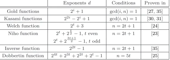
Table 1: Known APN power functionsxd _onF

2n

Exponentsd Conditions Proven in

Gold functions 2i

+ 1 gcd(i, n) = 1 [27,35] Kasami functions 22i

−2i

+ 1 gcd(i, n) = 1 [30,31] Welch function 2t

+ 3 n= 2t+ 1 [24] Niho function 2t

+ 2t2₋1,_teven _n= 2_t+ 1 [23]

2t

+ 23t2+1_−1,todd

Inverse function 22t

−1 n= 2t+ 1 [35] Dobbertin function 24t

+ 23t

+ 22t

+ 2t

−1 n= 5t [25]

In Table1, we list all known power APN mappings onF₂nwhich are known so far: The Welsh

and Niho functions are also AB, the Gold and Kasami functions are AB if nis odd. It is known that the inverse function and the Dobbertin function are not AB: The complete Walsh spectrum of the inverse function has been determined in [33], those of the Dobbertin function in [18], and these are not the spectra as defined in (3) and (2).

There are two questions which arise quite naturally:

Question 1. (1.) Is the list in Table1complete? (2.) Are all these examples “different”?

2

Equivalence of APN mappings

Let us begin with the second part of Question1. In order to describe whether two functionsFand

H are equivalent, we introduce group ring notation. This notion is also quite useful to describe the technique of “switching” an APN function. This is a very powerful tool to construct new APN functions, as we will show in this paper.

LetF_{be an arbitrary field, and let (G,+) be an additively written abelian group (we are only} interested in abelian groups, so we do not care about the general case). The group algebraF_[G] consists of all “formal” sums _X

g∈G

agg, ag∈F_.

We define componentwise addition X

g∈G

agg + X

g∈G

bgg := X

g∈G

(ag+bg)g,

and a multiplication

X

g∈G

agg · X

g∈G

bgg := X

g∈G

X

h∈G

ah·bg−h

!

g.

Together with these two operations and the scalar multiplicationλP_g∈Gagg:=P_g∈G(λag)g, the set F_{[G] becomes an algebra, the so calledgroup algebra. The dimension of this algebra as an} F_{-vectorspace is|G|. Given a function F:}F₂n_→F₂n_{, we associate a group algebra elementGF in} F_[F₂n_×F₂n_{] with it:}

GF := X

v∈Fn 2

(v, F(v)) in F_[F₂n_×F₂n_].

The coefficients of the group elements in GF are just 0 or 1 (more generally, any subset T of a groupGcan be identified with the elementP_g∈Tg, where the coefficients of all elements inT are 1). We have the following very easy Lemma:

Lemma 1. A functionF :F₂n_→F₂n _{is APN if and only if}

GF ·GF = 2n·(0,0) + 2·DF inC_[F₂n_×F₂n_{] (4)}

for some subsetDF ∈F₂n_×F₂n_.

In (4), we may replace C_{by any field of characteristic 6= 2 if we sayfor some subset DF ∈} Fn

2 ×F2n of size 2n−1·(2n−1).

We emphasize thatGis additively written, but this addition is quite different from the addition in the group algebra F_{[G]. If, for instance, A, B ⊂G andA∩B =∅, then A∪B is the subset} of G corresponding to A+B in F_{[G]. If g ∈ G, then A·g in} F_{[G] corresponds to the subset} {a+g : a∈A}. We callA·ga translateofA. It looks a bit awkward that the productA·gis the set ofsumsa+gwitha∈A.

The ideal generated byGF inF_2[F₂n_×F₂n_{] is a subspace of the 2}2n_{-dimensional vector space of} the group algebraF_2[F₂n_×F₂n_{]. The dimension is called the Γ-rankof the functionF. Similarly,} the dimension of the ideal generated byDF in F_2[F₂n_×F₂n_{] is called the ∆-rankof F.}

The Walsh transform of a functionF is nothing else than the Discrete Fourier transform of

GF, which we will describe briefly: If G is a finite abelian group, then there are |G| different homomorphisms χ : G → C_{, and the set of these homomorphisms (called characters) form a} group under multiplication χ1χ2(g) :=χ1(g)·χ2(g). This group is isomorphic toG. Characters

χmay be extended to homomorphismsχ:C_[G]→C_{[G] by linearity:}

χ(X

g∈G

agg) :=X

Let χ be a character of G, and Ψ an automorphism of G. Then the mapping χΨ _{: G → C} with χΨ_{(g) := χ(Ψ(g)) is again a character. Moreover, Ψ may be extended to a group algebra} automorphism. This shows that the Walsh spectrum of an elementD ∈C_{[G] is invariant under} the application of group automorphisms.

IfG=Fn

2 ×F2n, the characters are the mappingsχα,β defined byχα,β(u, v) := (−1)

tr(αu+βv)_,

where we identify the vector spaceFn

2 with the additive group of the finite fieldF2n. Therefore,

the Walsh spectrum is just the multi-set of character values ofGF.

Definition 1 (CCZ and EA equivalence, [14]). Two functionsF, H :F₂n _→F₂n _{are called CCZ}

equivalent if there is a group automorphism Ψ of F₂n_×F₂n _{and an element (u, v)∈} F₂n_×F₂n

such that

Ψ(GF) =GH·(u, v),

henceΨ(GF) is a translate ofGH. IfΨfixes the subgroup{(0, y) : y ∈F₂n_{} setwise, we say that}

the functions are EA equivalent(EA = extended affine equivalent). If, additionally, Ψfixes the set{(x,0) : x∈Fn

2 }, thenF andGare calledaffine equivalent.

We call this relationCCZ equivalentsince it has been first introduced (using different notation) by Carlet, Charpin and Zinoviev [19].

Proposition 1. If F is an APN (resp. AB) function, and if H is CCZ equivalent toF, then H

is also an APN (resp. AB) function.

Proof. LetGH = Ψ(GF)·(u, v). Ifχis a character ofF₂n_×F₂n_{, thenχ(GH) =χ}Ψ_{(GF)·χ(u, v),} hence the maximum absolute character value is invariant under CCZ equivalence, henceH is AB ifF isAB. IfF is APN, then

GF·GF =n·(0,0) + 2·DF

and therefore

GH·GH =n·(0,0) + 2·Ψ(DF) inC_[Fn 2 ×F2n].

This Proposition and its proof have some consequences: The Walsh spectrum isnotinvariant under CCZ equivalence: The Walsh coefficients χ(GF) and χ(GF)·χ(u, v) differ by the factor

χ(u, v), hence by ±1. The problem comes via the addition of the element (u, v): The Walsh spectrum is invariant under affine equivalence, but not under EA or CCZ equivalence. The set containing the Walsh spectrum and its negative is called the extended Walsh spectrum, and this is invariant under CCZ equivalence.

There is one drawback in the concept of CCZ equivalence: IfF is APN (or AB), the group algebra element Ψ(GF) does not necessarily correspond to a functionH, see [14], for instance.

It is obvious that the ∆- and Γ-ranks are invariant under CCZ equivalence.

Now we discuss the first part of Question1: Is the list in Table 1 complete? This has been answered negatively in [26]. One of the examples in [26] has been generalized to an infinite family, and a lot more constructions have been found since. In particular, Dillon [21] presented a list of 12 examples inF₂6_{. This list apppears in [8], together with many new examples in the cases}F₂7 andF₂8_.

However, all the new examples that have been constructed so far are “quadratic” in the sense that thederivativesF(x+a)−F(x) are linear mappings. Since the property of being “quadratic” is not invariant under CCZ equivalence (see [14]), we modify the definition as follows:

Definition 2. A functionF :F₂n_→F₂n _{isCCZ quadraticifF is CCZ equivalent to a function}

H with the property thatH(x+a)−H(x) is linear for alla∈F₂n_.

Definition 3 ([29]). Let F : F₂n _→ F₂n _{be an APN function. Then we define two incidence}

structures (designs) on the point set F₂n_×F₂n_{: In the first case, the blocks are the the sets}

GF·(a, b) :={(x+a, F(x) +b) : x∈Fn 2 }

for a, b∈Fn

2 , i.e. the translates ofGF. We call this design thedevelopment of GF, denoted by

dev(GF). Similarly, the design whose blocks are the translates

DF·(a, b)

of DF (see Lemma 1) is the development of DF, denoted by dev(DF). We call two designs

isomorphic if there is a permutation π on the set of points such that blocks (which are in our situation just subsets B = {g1, . . .} of the point set) are mapped to blocks (i.e. {π(g1, . . .} is a

block).

Any incidence structure gives rise to an incidence matrix: Rows and columns are indexed by the points and blocks, and the (p, B)-entry is 1 if the point p is incident with the blockB; the other entries are 0. The Γ-rank defined earlier is nothing else than the rank of the incidence matrix of dev(GF), considered as a matrix with entries inF_{2; similarly, the ∆-rank is the} F_{2-rank of an} incidence matrix of dev(DF).

Lemma 2. IfF andHare CCZ equivalent APN functions, then the designs dev(GF)and dev(GH)

are isomorphic. Moreover, the designs dev(DF)and dev(DH)are isomorphic.

Proof. Straightforward, see also [29]: The group automorphism Ψ with Ψ(GF) =GH·(u, v) is the permutation on the point set which maps blocks to blocks.

Using MAGMA [4] it is quite easy to determine the automorphism groups of these designs for small values of n. There is another group associated with the designs dev(GF) (resp. dev(DF)): The setsGF (resp. DF) are subsets ofF₂2n_{. Then there may exist automorphismsϕof}F₂2n _such that ϕ(GF) =GF ·(u, v) (resp. ϕ(DF) =DF·(u, v)) for someu, v∈F₂n_{. These automorphisms} form a groupcontainedin the automorphism group of the designs dev(GF) (resp. dev(DF)). Using notion adopted from the theory of difference sets, we call the group of these automorphisms the

multiplier group M(GF) (resp. M(DF)) of dev(GF) (resp. dev(DF)). It turns out that this group is much easier to compute with MAGMA than the full automorphism groups of the designs. We denote the group of translationsτa,b:Fn

2 ×F2n→F2n×F2n withτa,b(x, y) := (x+a, y+b) by T. Obviously, we have|T |= 22n_{, and|M(GF)∩ T |= 1 as well as|M(DF)∩ T |= 1.}

Since the multiplier group normalizesT, we have the following Lemma:

Lemma 3. Let F:Fn

2 →F2n be an APN function. Then

1. hM(GF),T i ⊆Aut(dev(GF)). 2. hM(DF),T i ⊆Aut(dev(DF)). 3. |M(GF)| ·22n_{=|hM(GF),T i|.}

4. |M(DF)| ·22n_{=|hM(DF),T i|.}

5. M(GF)⊆ M(DF).

It is possible to show thatM(GF) is just the automorphism group of the extended codeCFext

defined in the Introduction, see [8]. In all cases known to us, the “full” automorphism group of the design dev(GF) is just the multiplier group “times” the translationsτa,b.

We do not knwo whether this observation that holds for small values is true in general:

It seems that the automorphism group is a good invariant for CCZ equivalence, in particular to distinguish the quadratic from the non-quadratic case:

Theorem 4. If F : Fn

2 → F2n is an APN mapping such that F(x+a)−F(x) is linear for all

a∈Fn

2 , then the subgroup of the automorphism group of the development ofGF which is generated

by the translationsτa,b and the multipliers contains an elementary abelian group of order 23n_.

Proof. The mappings τa,b : F2n

2 → F22n with τa,b(x, y) = (x+a, y+b) are automorphisms of dev(GF), sinceτa,b(GF) =GF·(a, b). IfF is quadratic, then we may assume (after replacingF by a CCZ equivalent function, if necessary) that the mappingsLa(x) =F(x+a)+F(x)+F(a)+F(0) are linear. We compute

(La+Lb)(x) = F(x) +F(x+a) +F(a) +F(0) +F(x) +F(x+b) +F(b) +F(0) = F(x+a) +F(x+b) +F(a) +F(b).

Now we use

La(b+x) =F(a+b+x) +F(b+x) +F(a) +F(0)

and

La(b+x) =La(b) +La(x) =F(b) +F(a+b) +F(x) +F(a+x)

to obtain

F(a+b+x) =F(b+x) +F(a) +F(0) +F(b) +F(a+b) +F(x) +F(a+x). (5)

We get

La+b(x) = F(a+b+x) +F(a+b) +F(x) +F(0)

= F(b+x) +F(a) +F(b) +F(a+x) using (5) = La(x) +Lb(x).

This shows that the mappingsψa defined by ψa(x, y) = (x, y+La(x)) are linear, and

ψa(GF) = {(x, F(x) +La(x) : x∈F₂n_}

= {(x, F(x+a) +F(a) +F(0) : x∈Fn 2} = {(x−a, F(x) +F(a) +F(0) : x∈F₂n_} = GF·(−a, F(a) +F(0))

is a translate ofGF, hence the mappingsψa are automorphisms of dev(GF). Moreover,ψa+b = ψb◦ψa, hence the ψa’s form a group of order 2n. It is not difficult to see that the ψc together with the mappingsτa,b from a group of order 23n_.

Corollary 5. Under the assumptions of Theorem 4, the multiplier group M(GF) (equivalently the automorphism group of the extended codeCext

F ) has size divisible by2n, and both the orders of

Aut(dev(GF))and Aut(dev(DF))are divisible by 23n_.

Corollary 6 (G¨olo˘glu, Pott [29]). The Kasami power functions x13 _andx57 _onF7

2 are not CCZ

quadratic, hence they are not CCZ equivalent to quadratic functions.

Proof. Using MAGMA, it is easy to compute |Aut(dev(GF))| forF(x) = x13 _{and F(x) =x}157_: The order of the groups is, in both cases, 214_·7·(27_{−1) (Table6) which is not divisible by 2}21_.

Most people conjecture that the examples in Table1are all CCZ inequivalent, except for small

There is another concept related to quadratic APN functions: IfF is quadratic, then F(x+

a)−F(x) is linear, hence

Ha:={b : F(x+a)−F(x) =b for somex∈Fn

2} (6)

is an affine subspace. Ifa6= 0, this subspace has 2n−1_{elements (sinceF is APN), hence its is an} (affine) hyperplane. We say that a function iscrookedif the sets in (6) are (affine) hyperplanes for alla. This concept is due to Bending and Fon-der-Flaas [1]. “Crooked” is not invariant under CCZ equivalence, hence it would be better to say that a function F is crooked if it is CCZ equivalent to a function for which all the setsHa are hyperplanes:

Definition 4. An APN function F :F₂n _→F₂n _{is called CCZ crookedif F is CCZ equivalent}

to a function Gsuch that the sets

{b : G(x+a)−G(x) =bfor somex∈F₂n_}

are affine hyperplanes inF₂n_.

It is obvious that any (CCZ) quadratic function is (CCZ) crooked, and it is conjectured that the converse is also true, see [3,32] for partial results in this direction. However, as long as we do not know whether non-quadratic crooked functions may exist, we need to find arguments that a function is not CCZ crooked. The following argument gives an interesting necesary condition that a function is crooked:

Theorem 7. Let F :F₂n _→F₂n _{be an APN mapping. If F is CCZ crooked, then the dimension}

of the ideal generated by DF ∈F_2[F₂n_×F₂n_{] is at most 2}n+1_{, hence the ∆-rank is at most 2}n+1

(see Lemma 1for the definition ofDF).

Proof. IfF is crooked, there are 2n_{−1 (affine) hyperplanesHa such that} DF ={(a, x) : a∈F₂n_{\ {0}, x∈Ha}}

(replaceF by a CCZ equivalent function if necessary). We define

Ja :={(a, x) : x∈F₂n_}.

As explained above, these subsets may be also interpreted as elements inF_2[Fn

2 ×F2n]. We will show that the ideal generated byDF is contained in the subspaceI generated (as a vector space) by the 2n+1 _elements

{DF·(u,0) : u∈Fn

2 } ∪ {Ja : a∈F2n}.

It is sufficient to show that DF·(u, v) ∈ I for all (u, v)∈ Fn

2 ×F2n. The set corresponding to

DF ·(u, v) is{(a+u, Ha+v) : a∈F₂n_{}, whereHa+v={h+v : h∈Ha}. Here we have used} the notation (x, T) to denote the set of elements {(x, t) : t∈T}. Since Ha is a hyperplane, we haveHa+y=Ha orHa+yis the complement ofHa: In group algebra notation, this means for fixeda∈F₂n

(a+u, Ha+v) = (a+u, Ha)} or (a+u, Ha+v) = (a+u, Ha) +Ja+u

in F_2[F₂n_×F₂n_{]. In the equation above, we again identify subsets with the corresoponding group} algebra elements. Adding the elementJa+uhas the effect of complementingHa in (a+u, Ha).

Corollary 8. The Kasami power mappingsx13 _andx57 _onF7

2 are not CCZ crooked.

It would be very interesting to determine the ∆- and Γ-ranks of APN functions theoretically. In the next section (Theorem11), we will construct a new APN function which, at first view, seems to be non-quadratic. In order to prove that the function is indeed non-quadratic, we use Theorem 7 to show that the function cannot be CCZ equivalent to a crooked function, hence it cannot be quadratic. We may also use Theorem4to show that the function is non-quadratic, since the automorphism group of dev(GF) is too small for the new functionF. We have checked that our function is equivalent to the new example given in [7]. However, in that paper the authors erroneously claimed that their new function is CCZ equivalent to a quadratic one. Moreover, our function has been found independently from the search in [7].

3

The switching construction

The following interesting construction of an APN function is contained in [13]:

Proposition 2. The functionx3_+tr(x9_{)is APN inF}n

2.

This is a special case of what we will call “switching”. For this purpose, we consider certain projection homomorphisms on the group algebra F_{[G]. Let U be a subgroup of G. Then the} canonical homomorphismϕU :G→G/U defined byϕU(g) :=g+U can be extended by linearity to a homomorphismϕU :F_[G]→F_{[G/U]. LetD=}P_{aggbe an element in}F_{[G]. The coefficient} ofg+U in ϕ(D) is P_h∈g+Uah. If D has just coefficients 0 and 1, henceD corresponds to a set

D⊆G, then the coefficient ofg+U is|D∩(g+U)|. In particular, if each coset ofU meetsD in at most one element, thenϕU(D) has also just coefficients 0 and 1. This is the case ifU ≤ {0} ×Fn

2.

Definition 5(switching neighbours). LetF, H :Fn

2 →F2n be two functions, and letU ≤F2n×F2n

be a subgroup ofF₂n_×F₂n_{. We say that F andH are switching neighbours with respect to}

U ifϕU(GF) =ϕU(GH). We say that they areswitching neighbours in the narrow senseif

U ≤ {0} ×F₂n _{and dim(U) = 1.}

If F and H are switching neighbours with respect to U, we may obtain H from F by first

projecting GF ontoϕU(GF), and then we liftthis element to GH. We may also try to construct new switching neighboursH of F via such a project and lift procedure such that (hopefully) F

andH are CCZ inequivalent. This is in particular promising if the dimension ofU is small. The intuitive idea behind this approach is thatϕU(GF) isalmost an APN function, and so it may be easy to turn this “almost” APN into an APN function.

We will describe this approach (and applications) in the situation whereF : F₂n _→ F₂n _and

U ≤ {0} ×F₂n_{. This has the advantage that the coefficients ofϕU(GF) are just 0 and 1, since the} cosets of{0} ×F₂n _{(and therefore also the cosets ofU) meetGF no more than once. In this case,}

ϕU(GF) corresponds to a mappingFU :F₂n_→F₂n_/U′ _{with FU(v) :=v+U}′ _and

U′ _{={u : (0, u)∈U} (7)}

(henceU′ _{is basically the same asU).}

Proposition 3. Let F, H:Fn

2 →F2n, and let U ≤ {0} ×F2n. Then

FU =HU if and only if (0, F(v)−H(v))∈U for allv∈F₂n_.

If U ={(0,0),(0, u)}, then FU =HU if and only if there is a Boolean functionf :F₂n _→F_{2 such}

that H(v) =F(v) +f(v)·u.

Proof. We defineU′ _{as in (7). ThenFU(v) =HU(v) if and only ifF(v) +U}′_{=H(v) +U}′_{, hence}

FU(v)−HU(v)∈U′ _{for allv. This shows the first part of the proposition.} The function f is defined via

f(v) :=

0 ifF(v) =H(v) 1 ifF(v)6=H(v)

The two functionsF(x) =x3 _{andH(x) =x}3_+tr(x9_{) are switching neighbours in the narrow} sense: Take the 1-dimensional subspace U generated by (0,1) ∈ F₂n _×F₂n_{. Then ϕU(GF) =}

ϕU(GF).

Proposition3shows that we may obtain all switching neighbours ofF in the narrow sense (with respect to a one-dimensional subspace) by adding a Boolean functionf times a vectoru6= 0. Let

F be an APN function. The following Theorem gives a necessary and sufficient condition forf to produce another (not necessarily equivalent) APN function:

Theorem 9. Assume that F : Fn

2 → F2n is an APN function. Let u ∈ F2n, u 6= 0, and let

f :Fn

2 →F2be a Boolean function. Then F(v) +f(v)·uis an APN function if and only if

f(x) +f(x+a) +f(y) +f(y+a) = 0

for allx, y, a∈F₂n _with

F(x) +F(x+a) +F(y) +F(y+a) =u.

Proof. SinceF is APN, the equation

F(x+a) +F(x) + (f(x+a) +f(x))u=b

hat at most 4 solutions forx, namely thosexfor whichF(x+a) +F(x)∈ {b, b+u}. If there are 4 different solutionsx, y, x+a, y+a, then

F(x+a) +F(x) + (f(x+a) +f(x))u = b F(y+a) +F(y) + (f(y+a) +f(y))u = b.

But this is possible if and only if

F(x) +F(x+a) +F(y) +F(y+a) = u (8)

f(x) +f(x+a) +f(y) +f(y+a) = 1.

Remark 1. 1. The Boolean function f depends on u, i.e. for different choices of uwe may get different f’s.

2. It seems to be difficult to find a theoretical criteria that the functionF(v) +f(v)uis CCZ equivalent to F(v).

3. The functions F(v) and F(v) +f(v)u are switching neighbours in the narrow sense with respect to {(0,0),(0, u)}.

Theorem9immediately suggests a strategy to find Boolean functionsf such thatF(v) +f(v)u

is APN: Determine all 4-tuples x, y, x+y, y+asuch that (8) holds. These 4-tuples give rise to constraints

f(x) +f(x+a) +f(y) +f(y+a) = 0

We may viewf as a vector of length 2n _{(coordinates are indexed by elementsv in F}n

2, and the entries of the vector aref(v)). Thus the constraints are linear conditions, and we may findf’s by solving a system of linear equations.

Here is another interpretation: Write Fn

2 as direct sum U ⊕U. The functionF is uniquely determined by its function values. Consider the n-dimensional subspace V of F2n

2 spanned by {F(x) : x∈Fn

2}. WriteF2n as direct sum U ⊕U, this lifts to a decomposition of V =V′⊕V. So the evaluation off(v)uwill be in the 1-dimensional spaceV′_.

just an element of ˜V⊥_{. Moreover the functionsf(x)uin ˜V}⊥ _{in the same coset modulo V ⊆V˜}⊥ are CCZ equivalent (the difference is someAF,Abeing a linear mapF₂n_7→F_{2). So it is sufficient} to test onef(x)ufrom each coset.

So we know in particular that in the case that ˜V⊥ _{has dimensionn−1 there is no candidate} for a CCZ inequivalent switching function.

Definition 6. The finest equivalence relation on the set of APN functions such that all switching neighbours in the narrow sense and all EA-equivalent functions are equivalent, is called the EA switching equivalence relation. In the same way, we defineCCC switching equivalence.

This “switching idea” is closely related to a comment of John F. Dillon (which was motivated by [13]). Using the notion in Proposition3, he considered just the caseu= 1.

In the next section, we determine the EA switching equivalence classes of all known CCZ inequivalent APN functions onF₂n_{, n≤8. Several of the new constructions in the literature are} switching equivalent. It seems that the switching idea is quite powerful to construct new APN functions, since many of the new APN functions listed by Dillon in [8] are within just one switching class. In the casen= 8, the switching class of the Gold functionx3 _{contains 17 CCZ inequivalent} functions!

A more appropriate search would be to find all CCZ switching classes, which seems to be much harder than determining the EA switching classes.

4

Computational results and open problems

There is, up to equivalence, just one APN mapping F₂n _→ F₂n _{for n ≤4, hence no interesting} things happen in these cases. In the casen = 5, a complete classification of APN functions (up to CCZ equivalence) is contained in [6]. We summarize our computational results in the following tables. We also include some interesting CCZ invariants:

• ∆- and Γ-Rank.

• Orders of automorphism groups of dev(DF), dev(GF) andM(GF).

• extended Walsh spectrum.

If all these invariants are the same, we used a direct test to check that the examples are CCZ inequivalent, hence the reader can be sure that all the examples in the following tables are CCZ inequivalent. However, we do not claim that our tables are complete in the sense that they contain all possible CCZ equivalence classes of APN functions withn= 6,7 and 8.

We list the Walsh spectrum just if it is different from the Walsh spectrum ofx3_{. The Walsh} spectrum ofx3 _{is calledclassical.}

We number the examples as 1.1, 1.2, ..., 2.1, 2.2, ... etc. The first number describes the switching class, and the second number the CCZ inequivalent examples within this class. Our search was complete in the sense that, starting from the known APN functions, we searched through the entire switching class. Hence any new APN function must be a member of a new switching class. We used the examples in [21] and [8] as the starting cases.

Some comments about the sizes of the automorphism groups are in order: The automorphism groups contain the translationsτa,b, see Theorem 4, therefore we divided the group sizes in our tables by 22n_{. We were not able to determine the sizes of these groups ifn= 8. However, it was}

possible to determine the multiplier groupM(GF) of dev(GF): Using MAGMA, we determined the automorphism groups of the associated extended codesC_Fext. In the casesn≤7, the automorphism groups of dev(GF) have been always the groups generated by the multipliers plus the translations; therefore, it may be possible that the the group sizes in Table10desribe actually the sizes of the full automorphism groups.

It is quite interesting to look at the automorphism groups of the designs dev(GF), since they give some information aboutF:

Theorem 10. LetF(x)be an APN function onF₂n. Letv=|M(GF)|. Then the following holds:

(1.) If F(x)is quadratic, then2n _{divides v.}

(2.) If F is CCZ equivalent to a power mapping, then n·(2n_{−1) dividesv.}

(3.) If F is CCZ equivalent to a polynomial inF_{2[x], thenndivides v.}

Proof. The first statement is simply Theorem4. IfF(x)∈ F_{2[x], then the mapping}F₂n →F₂n

defined by (x, y)7→(x2, y2) has ordern, and it fixes the setGF. This shows (3). IfF(x) =γ·xd, then the 2n−1 mappings defined by (x, y)7→(αx, αd·y),α∈F₂n, fix the setGF. Moreover, we

may assume thatγ= 1, otherwise we replaceF by the CCZ equivalent function 1

γF, which shows

(2).

We did mention already that quadratic functions are crooked. The following question is of interest:

Question 3. Are all crooked functions quadratic?

A function defined by P_i,jαi,jx2i₊₂j

is quadratic. Therefore, Theorems 10 and 7 show the following:

Remark 2. The only non-quadratic functions in Tables 3,5 and7are the function no. 2.12 in Table3and the functions no. 5.1,6.1 and 7.1 in 7. Moreover, none of these functions is crooked.

We note that our new function 14.3 in Table7is inequivalent to a polynomial with coefficients inF_{2(Theorem10).}

We note that Table 3 contains, up to CCZ-equivalence, all APN functions on F₂5_{. In the} tables (5), (7) and (9), we only claim that we did apply the switching construction recursively to all known APN functions, in particular to those given by Dillon. In Table (5), the Example 2.12 is new (see Theorem11), and in Table (7), the Example 14.3 is new. However, we did not apply the switching construction to all the memebers of the CCZ equivalence classes. In other words, we started with the functions listed in the tables below, and we determined the EA switching classes,

notthe CCZ switching classes.

In our opinion, the most interesting function is the following non-quadratic example, see also [7]:

Theorem 11. Let F₂6 be the finite field which is constructed as the splitting field of x6+x4+

x3_{+x+ 1∈F}

2[x]. Letu be a root of this polynomial in F26. Then the function F :F₂6 →F₂6

with

F(x) = x3_+u17_(x17_+x18_+x20_+x24_{) +u}18_x9_+u36_x18_+u9_x36_+x21_+x42₊ +tr_(u27_x+u52_x3_+u6_x5_+u19_x7_+u28_x11_+u2_x13₎ (9)

is an APN function which is a switching neighbour of Function 2.4 in Table 5. This function cannot be CCZ equivalent to a crooked function.

Proof. One may quite easily check that the function is APN. One may also show that it is a switching neighbour ofx3_+u17_(x17_+x18_+x20_+x24_{). Note that the ∆-rank 152> 2}7 _{of this} function is too big for a crooked function, see Theorem7.

Remark 3. The functionF(x) in (9) may be also written

F(x) = x3+u17(x17+x18+x20+x24) +

u14(tr(u52x3+u6x5+u19x7+u28x11+u2x13) +tr8/2((u2x)9) +tr4/2(x21))

wheretr_8/2 andtr_4/2 denote the relative traceF_8→F_{2 and}F_4→F_{2. Note that (u}2_x)9_∈F_{8 and}

x21_∈F

Two APN functions which are switching equivalent in the narrow sense are quite “similar”, they are “almost” equal (see Proposition3). Therefore, the following question seems natural:

Question 4. Is there some property which distinguishes switching equivalent functions from those which are not switching equivalent?

Our computational results are quite pessimistic regarding this question. It seems that there is no property of an APN function which is preserved under switching. Also the sizes of the equivalence classes seem to behave “strange”: In then= 8 case, there is one large switching class, but in the casen= 7 there are only small classes.

It seems that many inequivalent APN functions exist. So, in our opinion, the main question about APN functions is to determine at least a lower bound for the number of inequivalent ones. Let APN(n) denote the number of CCZ inequivalent APN functionsF₂n_→F₂n_{. Then we ask:}

Question 5. Does the function APN(n) grows exponentially?

This paper contains a new non-quadratic APN function. We think that it is worth to search for more examples:

Problem 1. Find more nonquadratic APN functions.

We described the switching construction in quite a general form, and then we specialized to the case of 1-dimensional subspaces U ≤ {0} ×Fn

2 . In this case, it was (rather) easy to find switching neighbours. But of course one may also use higher-dimensional subspaces, or one may use subspaces not contained in{0} ×Fn

2 . It will be more difficult to handle these cases, but we do not think that it is hopeless. IfU becomes larger, the projections are further away from being APN, therefore the “lifting” will become more difficult. On the other hand, if we are using higher-dimensional subspacesU, we obtain more freedom for the lifting. But ifU is too big, the approach will most likely become useless: If, in the extremal case, U ={0} ×F₂n_{, then all APN} functionsF project onto the same setϕU(GF).

A generalization of the switching idea to functions between fields of odd characteristic is obvi-ous. Therefore, one may also apply this approach to PN functions:

Problem 2. Try to use the switching idea for other subspacesU or for PN functions.

Finally, we come back to the original motivation for studying APN functions: APN’s are used in cryptography because they are highly nonlinear. Moreover, functions used in cryptography should quite often have large algebraic degree. Therefore, quadratic functions are usually “weak” regarding applications. But our paper shows that functions of large degree can be quite similar to quadratic (i.e. weak) functions via our projection idea. Therefore, it may be worth to see whether “switching” can be used for cryptanalysis.

In the following tables, it is important to know the primitive element that we have used to construct the finite fields. In Table 2, we list these polynomials p(x). The primitive element u

Table 2: Used primitive polynomialsp(x)

n p(x)

6 x6_+x4_+x3_{+x+ 1} 7 x7_{+x+ 1}

8 x8_+x4_+x3_+x2_{+ 1}

Table 3: All switching classes of APN’s inF₂5

n= 5 No. F(x) 1.1 x3 1.2 x5 2.1 x−1

Table 4: Invariants of switching classes in Table3

n= 5

No. Γ-rank ∆-rank |Aut(dev(GF))|/210 _{|Aut(dev(DF))|/2}10 _{Walsh spectrum}

1.1 330 42 25_{·5·31 2}5_{·5·31 classical}

1.2 330 42 25_{·5·31 2}10_{·5·31 classical} 2.1 496 232 2·5·31 2·5·31 non-classical, see [33]

Table 5: Known switching classes of APN’s inF6 2

n= 6 No. No. in [8] F(x)

1.1 1 x3

1.2 2 x3

+u11

x6 +ux9

2.1 3 ux5

+x9 +u4

x17 +ux18

+u4

x20 +ux24

+u4

x34 +ux40

2.2 4 u7

x3 +x5

+u3

x9 +u4

x10 +x17

+u6

x18

2.3 5 x3

+ux24 +x10

2.4 6 x3

+u17 (x17

+x18 +x20

+x24 )

2.5 7 x3

+u11

x5 +u13

x9 +x17

+u11

x33 +x48

2.6 8 u25

x5 +x9

+u38

x12 +u25

x18 +u25

x36

2.7 9 u40

x5 +u10

x6 +u62

x20 +u35

x33 +u15

x34 +u29

x48

2.8 10 u34

x6 +u52

x9 +u48

x12 +u6

x20 +u9

x33 +u23

x34 +u25

x40

2.9 11 x9

+u4 (x10

+x18 ) +u9

(x12 +x20

+x40 )

2.10 12 u52

x3 +u47

x5 +ux6

+u9

x9 +u44

x12 +u47

x33 +u10

x34 +u33

x40 2.11 13 u(x6

+x10 +x24

+x33 ) +x9

+u4

x17

Table 6: Known switching classes of APN’s inF6

2: Invariants

n= 6 No. Γ-rank ∆-rank |Aut(dev(GF))|/2

12

|Aut(dev(DF))|/2

12

Walsh spectrum

1.1 1102 94 27

·33

·7 28

·33

·7 classical

1.2 1146 94 26

·32

·7 27

·32

·7 classical

2.1 1158 96 26

·5 26

·5 classical

2.2 1166 94 26

·7 27

·7 classical

2.3 1166 96 27

·7 27

·7 classical

2.4 1168 96 26

26

classical

2.5 1170 96 26

·5 26

·5 {0(1), −8(1176), 8(1512), 0(1071), 16(210), −16(126), 64(1)}

2.6 1170 96 26

26

classical

2.7 1170 96 26

26

classical

2.8 1170 96 26

26

classical

2.9 1172 96 26

26

classical

2.10 1172 96 26

26

classical

2.11 1174 96 26

26

classical

2.12 1300 152 23

23

classical

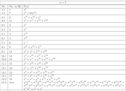
Table 7: Known switching classes of APN’s inF₂7

n= 7 No. No. in [8] F(x)

1.1 1 x3

1.2 7 x3

+tr_(x9₎

2.1 8 x34

+x18 +x5

2.2 11 x3

+x17 +x33

+x34

3.1 3 x5

4.1 2 x9

5.1 4 x13

6.1 5 x57

7.1 6 x−1

8.1 9 x65

+x10 +x3

9.1 13 x3

+x9 +x18

+x66

10.1 14 x3

+x12 +x17

+x33

10.2 10 x3

+x17 +x20

+x34 +x66

11.1 15 x3

+x20 +x34

+x66

12.1 16 x3

+x12 +x40

+x72

13.1 12 x3

+x5 +x10

+x33 +x34

14.1 17 x3

+x6 +x34

+x40 +x72

14.2 18 x3

+x5 +x6

+x12 +x33

+x34

14.3 new u2

x96 +u78

x80 +u121

x72 +u49

x68 +u77

x66 +u29

x65 +u119

x48 +u117

x40 +u28

x36 + u107

x34 +u62

x33 +u125

x24 +u76

x20 +u84

x18 +u110

x17 +u49

x12 +u102

x10 +u69

x9 + u14

x6 +x5

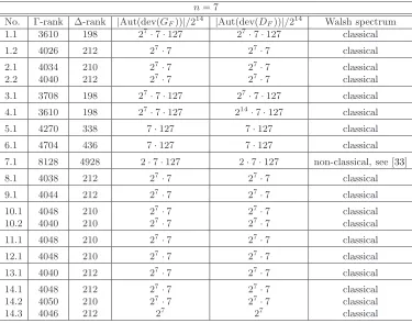
Table 8: Known switching classes of APN’s inF₂7_{: Invariants}

n= 7 No. Γ-rank ∆-rank |Aut(dev(GF))|/2

14

|Aut(dev(DF))|/2

14

Walsh spectrum

1.1 3610 198 27

·7·127 27

·7·127 classical

1.2 4026 212 27

·7 27

·7 classical

2.1 4034 210 27

·7 27

·7 classical

2.2 4040 212 27

·7 27

·7 classical

3.1 3708 198 27

·7·127 27

·7·127 classical

4.1 3610 198 27

·7·127 214

·7·127 classical

5.1 4270 338 7·127 7·127 classical

6.1 4704 436 7·127 7·127 classical

7.1 8128 4928 2·7·127 2·7·127 non-classical, see [33]

8.1 4038 212 27

·7 27

·7 classical

9.1 4044 212 27

·7 27

·7 classical

10.1 4048 210 27

·7 27

·7 classical

10.2 4040 210 27

·7 27

·7 classical

11.1 4048 210 27

·7 27

·7 classical

12.1 4048 210 27

·7 27

·7 classical

13.1 4040 212 27

·7 27

·7 classical

14.1 4048 212 27

·7 27

·7 classical

14.2 4050 210 27

·7 27

·7 classical

14.3 4046 212 27

27

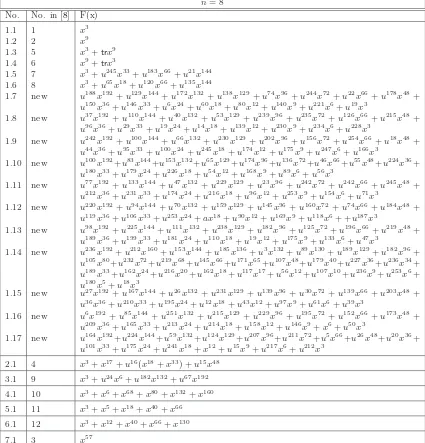
Table 9: Known switching classes of APN’s inF8 2

n= 8 No. No. in [8] F(x)

1.1 1 x3

1.2 2 x9

1.3 5 x3

+tr_x9

1.4 6 x9

+trx3

1.5 7 x3

+u245

x33 +u183

x66 +u21

x144

1.6 8 x3

+u65

x18 +u120

x66 +u135

x144

1.7 new u188

x192 +u129

x144 +u172

x132 +u138

x129 +u74

x96 +u244

x72 +u22

x66 +u178

x48 + u150

x36 +u146

x33 +u6

x24 +u60

x18 +u80

x12 +u140

x9 +u221

x6 +u19

x3

1.8 new u37

x192 +u110

x144 +u40

x132 +u53

x129 +u239

x96 +u235

x72 +u126

x66 +u215

x48 + u96

x36 +u29

x33 +u19

x24 +u14

x18 +u139

x12 +u230

x9 +u234

x6 +u228

x3

1.9 new u242

x192 +u100

x144 +u66

x132 +u230

x129 +u202

x96 +u156

x72 +u254

x66 +u18

x48 + u44

x36 +u95

x33 +u100

x24 +u245

x18 +u174

x12 +u175

x9 +u247

x6 +u166

x3

1.10 new u100

x192 +u83

x144 +u153

x132 +u65

x129 +u174

x96 +u136

x72 +u46

x66 +u55

x48 +u224

x36 + u180

x33 +u179

x24 +u226

x18 +u54

x12 +u168

x9 +u89

x6 +u56

x3

1.11 new u77

x192 +u133

x144 +u47

x132 +u229

x129 +u23

x96 +u242

x72 +u242

x66 +u245

x48 + u212

x36 +u231

x33 +u174

x24 +u216

x18 +u96

x12 +u253

x9 +u154

x6 +u71

x3

1.12 new u220

x192 +u94

x144 +u70

x132 +u159

x129 +u145

x96 +u160

x72 +u74

x66 +u184

x48 + u119

x36 +u106

x33 +u253

x24 +ax18

+u90

x12 +u169

x9 +u118

x6

+ +u187

x3

1.13 new u98

x192 +u225

x144 +u111

x132 +u238

x129 +u182

x96 +u125

x72 +u196

x66 +u219

x48 + u189

x36 +u199

x33 +u181

x24 +u110

x18 +u19

x12 +u175

x9 +u133

x6 +u47

x3

1.14 new u236

x192 +u212

x160 +u153

x144 +u185

x136 +u3

x132 +u89

x130 +u189

x129 +u182

x96 + u105

x80 +u232

x72 +u219

x68 +u145

x66 +u171

x65 +u107

x48 +u179

x40 +u227

x36 +u236

x34 + u189

x33 +u162

x24 +u216

x20 +u162

x18 +u117

x17 +u56

x12 +u107

x10 +u236

x9 +u253

x6 + u180

x5 +u18

x3

1.15 new u27

x192 +u167

x144 +u26

x132 +u231

x129 +u139

x96 +u30

x72 +u139

x66 +u203

x48 + u36

x36 +u210

x33 +u195

x24 +u12

x18 +u43

x12 +u97

x9 +u61

x6 +u39

x3

1.16 new u6

x192 +u85

x144 +u251

x132 +u215

x129 +u229

x96 +u195

x72 +u152

x66 +u173

x48 + u209

x36 +u165

x33 +u213

x24 +u214

x18 +u158

x12 +u146

x9 +x6

+u50

x3

1.17 new u164

x192 +u224

x144 +u59

x132 +u124

x129 +u207

x96 +u211

x72 +u5

x66 +u26

x48 +u20

x36 + u101

x33 +u175

x24 +u241

x18 +x12

+u15

x9 +u217

x6 +u212

x3

2.1 4 x3

+x17 +u16

(x18 +x33

) +u15

x48

3.1 9 x3

+u24

x6 +u182

x132 +u67

x192

4.1 10 x3

+x6 +x68

+x80 +x132

+x160

5.1 11 x3

+x5 +x18

+x40 +x66

6.1 12 x3

+x12 +x40

+x66 +x130

Table 10: Known switching classes of APN’s inF8

2: Invariants

n= 8

No. Γ-rank ∆-rank |M(GF))| Walsh spectrum

1.1 11818 420 211

·255 classical

1.2 12370 420 211

·255 classical

1.3 13800 432 211

·3 classical

1.4 13804 434 211

·3 classical

1.5 13842 436 210

·3 classical

1.6 13848 438 210

·3 classical

1.7 14034 438 28

·3 classical

1.8 14032 438 210

·3 classical

1.9 14036 438 210

·3 classical

1.10 14036 438 29

·3 classical

1.11 14032 438 210

·3 classical

1.12 14034 438 210

·3 classical

1.13 14030 438 29

·3 classical

1.14 14046 454 29

classical

1.15 14036 438 28

·3 classical

1.16 14032 438 29

·3 classical

1.17 14028 438 29

·3 classical

2.1 13200 414 210

·32

·5 classical

3.1 14024 438 210

·3 classical

4.1 14040 454 211

classical

5.1 14044 446 211

classical

6.1 14046 438 211

classical

7.1 15358 960 23

References

[1] T. D. Bending and D. Fon-Der-Flaass,Crooked functions, bent functions, and distance

regular graphs, Electron. J. Combin., 5 (1998), pp. Research Paper 34, 14 pp. (electronic).

[2] T. Beth, D. Jungnickel, and H. Lenz, Design Theory, Cambridge University Press,

Cambridge, 2 ed., 1999.

[3] J. Bierbrauer and G. M. Kyureghyan, Crooked binomials, Des. Codes Cryptogr., 46

(2008), pp. 269–301.

[4] W. Bosma, J. Cannon, and C. Playoust, The Magma algebra system. I. The user

lan-guage. J. Symbolic Comput., 24(3-4):235-265, 1997

[5] C. Bracken, E. Byrne, N. Markin, and G. McGuire, Quadratic almost perfect

non-linear functions with many terms. IACR Cryptology ePrint Archive: 2007/115, 2007.

[6] M. Brinkmann and G. Leander,On the classification of APN functions up to dimension

five, in Abstract Book of the Workshop on coding and cryptography, N. S. D. Augo and J.-P. Tillich, eds., INRIA, 2007, pp. 39–48.

[7] , On the classification of apn functions up to dimension five, Des., Codes, Cryptogr., (2008).

[8] K. Browning, J. Dillon, R. Kibler, and M. McQuistan,APN polynomials and related

codes. submitted, 2008.

[9] A.E. Brouwer and L.M.G.M. Tolhuizen,A Sharpening of the Johnson Bound for Binary

Linear Codes, Designs, Codes and Cryptography, Vol. 3, No. 1 (1993) pp. 95-98.

[10] L. Budaghyan and C. Carlet,Classes of quadratic APN trinomials and hexanomials and

related structures. IACR Cryptology ePrint Archive: 2007/098, 2006.

[11] L. Budaghyan, C. Carlet, and G. Leander, A class of quadratic APN binomials

in-equivalent to power functions. IACR Cryptology ePrint Archive: 2006/445, 2006.

[12] , Another class of quadratic APN binomials over F2n: the case n divisible by 4, in

Abstract Book of the Workshop on coding and cryptography, N. S. D. Augo and J.-P. Tillich, eds., INRIA, 2007, pp. 49–58.

[13] ,Constructing new APN functions from known ones.http://eprint.iacr.org/, 2007.

[14] L. Budaghyan, C. Carlet, and A. Pott,New classes of almost bent and almost perfect

nonlinear polynomials, IEEE Trans. Inform. Theory, 52 (2006), pp. 1141–1152.

[15] L. Budaghyan and T. Helleseth,New perfect nonlinear monomials overfp2k for any odd

prime p. to be presented at SETA ’08.

[16] E. Byrne, C. Bracken, N. Markin, and G. McGuire, New families of quadratic

almost perfect nonlinear trinomials and multinomials. preprint, available online at:

http://mathsci.ucd.ie/∼gmg/, 2007.

[17] E. Byrne and G. McGuire,Certain new quadratic APN functions are not APN infinitely

often, in Abstract Book of the Workshop on coding and cryptography, N. S. D. Augo and J.-P. Tillich, eds., INRIA, 2007, pp. 59–68.

[18] A. Canteaut, P. Charpin, and H. Dobbertin,Weight divisibility of cyclic codes, highly

nonlinear functions on F2m, and crosscorrelation of maximum-length sequences, SIAM J.

[19] C. Carlet, P. Charpin, and V. Zinoviev,Codes, bent functions and permutations suitable for DES-like cryptosystems, Des. Codes Cryptogr., 15 (1998), pp. 125–156.

[20] J. Dillon and H. Dobbertin, New cyclic difference sets with Singer parameters., Finite

Fields Appl., 10 (2004), pp. 342–389.

[21] J. F. Dillon. slides from talk given at ”Polynomials over Finite Fields and Appliocations”,

held at Banff International Research Station, 2006.

[22] C. Ding and J. Yuan,A new family of skew Paley-Hadamard difference sets, J. Comb.

The-ory Ser.A, 113 (2006), pp. 1526–1535.

[23] H. Dobbertin, Almost perfect nonlinear power functions on GF(2n_{): The Niho case,}

Infor-mation and Computation, 151 (1999), pp. 57–72.

[24] , Almost perfect nonlinear power functions on GF(2n_{): the Welch case, IEEE Trans.}

Inform. Theory, 45 (1999), pp. 1271–1275.

[25] ,Almost perfect nonlinear power functions on GF(2n_{): A new case forndivisible by5, in}

Proceedings of the conference on Finite Fields and Applications, Augsburg 1999, D. Jungnickel and H. Niederreiter, eds., Berlin, 2001, Springer-Verlag, pp. 113–121.

[26] Y. Edel, G. Kyureghyan, and A. Pott,A new APN function which is not equivalent to

a power mapping, IEEE Trans. Inform. Theory, 52 (2006), pp. 744–747.

[27] R. Gold, Maximal recursive sequences with 3-valued recursive cross-correlation function,

IEEE Trans. Inf. Th., 14 (1968), pp. 154–156.

[28] S. W. Golomb and G. Gong, Signal design for good correlation, Cambridge University

Press, Cambridge, 2005. For wireless communication, cryptography, and radar.

[29] F. G¨olo˘glu and A. Pott, Almost perfect nonlinear functions: A possible geometric

ap-proach (25 pages). Presented at Academic Contact ForumCoding Theory and Cryptography, Brussels, 2008.

[30] H. Janwa and R. M. Wilson, Hyperplane sections of Fermat varieties in P3 _{in char.2}

and some applications to cyclic codes, in Applied algebra, algebraic algorithms and error-correcting codes (San Juan, PR, 1993), vol. 673 of Lecture Notes in Comput. Sci., Springer, Berlin, 1993, pp. 180–194.

[31] T. Kasami,The weight enumerators for several classes of subcodes of the 2nd order binary

Reed-Muller codes, Information and Control, 18 (1971), pp. 369–394.

[32] G. M. Kyureghyan, Crooked maps inF₂n, Finite Fields Appl., 13 (2007), pp. 713–726.

[33] G. Lachaud and J. Wolfmann,The weights of the orthogonals of the extended quadratic

binary Goppa codes, IEEE Trans. Inform. Theory, 36 (1990), pp. 686–692.

[34] R. Lidl and H. Niederreiter,Finite Fields, vol. 20 of Encyclopedia of Mathematics and

its Applications, Cambridge University Press, 2nd ed., 1997.

[35] K. Nyberg,Differentially uniform mappings for cryptography, in Advances in Cryptography.

EUROCRYPT’93, vol. 765 of Lecture Notes in Computer Science, New York, 1994, Springer-Verlag, pp. 55–64.

[36] Z. Zha, G. M. Kyureghyan, and X. Wang,A new family of perfect nonlinear binomials.