Analysis of the Parallel
Distinguished Point Tradeoff
⋆Jin Hong1, Ga Won Lee1, and Daegun Ma2
1
Seoul National University, Seoul, Korea
{jinhong,gwlee87}@snu.ac.kr 2
Konkuk University, Seoul, Korea [email protected]
Abstract. Cryptanalytic time memory tradeoff algorithms are tools for quickly inverting one-way functions and many consider the rainbow ta-ble method to be the most efficient tradeoff algorithm. However, it was recently announced, mostly based on experiments, that the paralleliza-tion of the perfect distinguished point tradeoff algorithm brings about an algorithm that is 50% more efficient than the perfect rainbow table method. Motivated by this claim, we provide an accurate theoretic anal-ysis of the parallel version of the non-perfect distinguished point tradeoff algorithm.
Performance differences between different tradeoff algorithms are usu-ally not very large, but even these small differences can be crucial in practice. So we take care not to ignore the side effects of false alarms while analyzing the online time complexity of the parallel distinguished point tradeoff algorithm. Our complexity results are used to compare the parallel non-perfect distinguished point tradeoff against the non-perfect rainbow table method. The two algorithms are compared under identical success rate requirements and the pre-computation efforts are taken into account. Contrary to our anticipation, we find that the rainbow table method is superior in typical situations, even though the parallelization did have a positive effect on the efficiency of the distinguished point tradeoff algorithm.
Keywords: time memory tradeoff, parallel distinguished point, distin-guished point, rainbow table
1
Introduction
Cryptanalytic time memory tradeoff algorithms are tools for quickly inverting one-way functions with the help of pre-computed tables. By changing the algo-rithm parameters, one is able to balance the size of the stored pre-computed table against the average time required for each inversion. The tradeoff tech-niques are typically used to recover passwords from the information of password hashes and there are commercial implementations which allow one to defeat the
⋆
access control mechanisms that are embedded in widely used document file for-mats. The tradeoff technique is not only used among hackers, but is also an important tool for the law enforcement agencies.
It has long been known that the tradeoff attacks can be prevented by design-ing the security system to incorporate what are referred to as randomsalts, but there still are many systems in use today that do not incorporate this counter-measure, and the only obstacle in applying the tradeoff attacks to these systems is the large pre-computation requirement. However, as was shown in [12], even this barrier is lowered when the security ultimately relies on human generated passwords. Hence, many current security systems are susceptible to the trade-off attacks, and finding the exact capabilities and limitations of the tradetrade-off algorithms remains an interesting subject of study.
The first explicit time memory tradeoff algorithm was invented by Hell-man [8]. Shortly thereafter, the distinguished point (DP) technique was intro-duced. This idea, attributed to Rivest in [7], greatly reduces the table lookup re-quirements of Hellman’s original algorithm. The tradeoff algorithm most widely known to the public today is the rainbow table method [13]. When the search space size isN, a typical tradeoff algorithm allows storage requirementM and inversion time T to be balanced, subject to the equationT M2≈N2, through
the choice of associated parameters. Rough analyses of the tradeoff algorithms show that the tradeoff coefficient Xtc = T M2/N2 is close to 1 for reasonable
choices of parameter sets. However, it is different for each algorithm and does change with the choice of the parameter set.
The tradeoff coefficientXtcis a measure of how efficiently an algorithm
bal-ances storage against online time, with a smaller number corresponding to better tradeoff efficiency. In a recent work [11], that builds on the works [1, 10], the value ofXtcwas accurately computed for the Hellman, DP, and rainbow tradeoffs, and
then the tradeoff coefficients of the three algorithms were compared against each other. Unlike previous attempts, the comparison of [11] took the inversion suc-cess rate, pre-computation cost, and the number of bits required to store each table entry fully into account. Their conclusion, in oversimplified terms, was that the classical Hellman and the DP tradeoffs perform comparable to each other and that the rainbow table method outperforms these two. Even though this was in agreement with what many had believed for some time, the performances of the algorithms were shown to be quite close to each other for moderate success rates, justifying the need for such careful analyses before any comparison.
The conclusions are that parallelization has a positive effect, not only on the wall-clock running time, but also on the combined processor time of the DP tradeoff. However, for typical range of parameters, the gain in performance ob-tained is shown to be insufficient to overcome the superiority of the rainbow table method over the DP tradeoff. If the wall-clock running time is more important than the total processor time, depending on the degree of parallelism available, there can be situations where the parallel DP tradeoff is desirable over the rain-bow tradeoff. However, if the combined processor time is more important, one should use the rainbow method rather than the parallel DP method.
Our analysis may be seen as theoretic or practically limited in two respects. First, the above mentioned combined processing time may not directly corre-spond to the real-world cost of running an algorithm, but this issue is clearly outside the scope of this paper. Second, we do not discuss whether implement-ing the parallel DP tradeoff is practical on various specific platforms. In fact, the demand for online memory by the parallel DP tradeoff is higher than other tradeoff algorithms and this could be critical in certain environments. However, aside from issues that are specific to implementation environments, we are as practical as possible in treating the two compared algorithms, in that the success probabilities, pre-computation costs, and bits required per table entry are taken into account during algorithm comparison.
We acknowledge that parallel processing of tradeoff tables is not a new idea. Distributed key search with a central pre-computation table repository is men-tioned in [2, 3] as an application for DP tradeoffs. It was noted in [13] that processing multiple rainbow tables in parallel will reduce the total combined processor time. In fact, the rainbow tradeoff is usually taken to process its ta-bles in parallel, even though the number of its tata-bles is much smaller than that of the DP tradeoff and allows lower degree of straightforward parallelization. In [10] one can find a very rough heuristic argument as to why the classical Hellman tradeoff will not benefit from parallelization. Finally, the work [9, 14] claims that the parallel version of the perfect3 DP tradeoff is twice as efficient as the perfect rainbow table method, mainly based on experiment results.
The current work was motivated by the above mentioned [14], which an-nounced the perfect table parallel DP tradeoff as the “New World Champion” of tradeoff algorithms. However, all the algorithms considered in this paper are the non-perfect table versions. Let us explain our choice to analyze the non-perfect table version of the parallel DP tradeoff rather than the perfect table version.
The perfect DP tradeoff was first studied in [2, 3]. They left some unresolved problems and many view [15] as completing the analysis. However, the analysis of [15] does not provide figures that are accurate enough for use in this paper as data representing the performance of a competing algorithm. For example, an entry in Table 2 of the paper gives 21.6425 and 21.1357 as experimental and corresponding theoretic figures concerning a certain storage count. On the
3
surface, the two values seem to be in good agreement, but one must note that they are presented in logarithmic scale. We cannot explain the details here, but when the two storage figures representing experiment and theory are translated to tradeoff efficiency figures, they become the ratio 222121.1357.6425
2
≈2.02. Theoretic result of such inaccuracy may be acceptable for many applications, but is not appropriate for the purpose of comparing different algorithms, since algorithm performances are likely to differ by a comparable ratio.
A perfect DP table is obtained by removing redundancies present in a non-perfect DP table and this implies that each non-perfect table requires more pre-computation to construct than the non-perfect version, if the two are to bring about the same success rate. Even though the perfect table DP tradeoff is ex-pected to be more efficient than the non-perfect table version, with the current state of knowledge explained above, it is hard to judge whether the degree of enhancement in efficiency justifies the additional pre-computation involved.
Since the state of current knowledge is far from ready for the treatment of perfect table parallel DP tradeoffs, and since it is unclear if the efficiency advantage of the perfect version will be worth the higher pre-computation cost, the non-perfect table parallel DP tradeoff is treated in this paper. The perfect table parallel DP tradeoff is certainly of interest and is left as a subject of future study, which can be approached only after a more accurate analysis of the perfect table (serial) DP tradeoff has been developed. The initial view of the effects of parallelism we obtain and the method of approaching we develop in dealing with the non-perfect case will be of guidance in studying the perfect case.
The rest of this paper is organized as follows. We fix the basic terminology and recall some previous results in Section 2. The parallel DP tradeoff algorithm is made explicit in Section 3 and its theoretic analysis is given in Section 4. After verifying our theoretic developments with experiments in Section 5, the efficiency figures obtained through our analysis are compared against those of the original DP and rainbow table methods in Section 6. The final section contains a summary of our results. Most of the technical proofs are deferred to the appendix.
2
Preliminaries
Throughout this paper F : N → N will be a function acting on a set N of sizeN. As is done by any theoretic analysis of tradeoff algorithms, we takeF to be the random function during our theoretic arguments.
password recovery from sufficiently long password hashes are to be considered, the second version is the correct inversion problem to study [11]. In the interest of practical applicability, the current paper deals with the second inversion problem.
Terminology. We assume that the reader has basic knowledge of the DP and rainbow tradeoff algorithms. Below, we quickly review the terminology and fix notation, mainly focusing on the DP tradeoff, but analogous terminology and no-tation will be used with the rainbow tradeoff. All tradeoff algorithms considered in this paper are the non-perfect table versions.
The correct answer to be recovered and the inversion target will always be denoted by xandy=F(x), respectively. EachDP table, consisting of starting and ending point pairs of pre-computedDP chains, will contain approximately m entries. What is meant by the term approximately will be explained below. The probability of DP occurrence is set to 1
t, so that the average chain length
is roughlyt. We distinguish between a DP table and aDP matrix, which is the complete set of m pre-computed chains. An online chain merging into a pre-computation chain will bring about a false alarm. We omit any mentioning of reduction functions, as our arguments will mostly focus on a single table. Rather than using exactlyttables, we allow more flexibility and useℓtables, whereℓ≈t. Flexibility is also given to the matrix stopping rule, so thatmt2=D
mscN, with
amatrix stopping constant Dmsc≈1. The conditionDmsc≈1 can be justified as
was originally done by Hellman [8] or through a birthday paradox argument as given in [5, 6]. In all cases, we assume that the parameters are reasonable in the sense that m, t≫0, which, in particular, implies t≪√N through the matrix stopping rule.
Any implementation of the DP tradeoff will place achain length bound ˆt to detect chains falling into loops that do not contain DPs. If one generates m0
chains with the chain length bound ˆt, one can expect to collectm0{1− 1−1t ˆ t }
DP chains. Rather than requiring a DP table to contain the information of exactlymDP chains, we take the approach that the chains are always generated fromm0=m/{1− 1−1t
ˆ t
}starting points and that the resulting approximately mDP chains are accounted for by each DP table.
Note that the expected number of chains that do not reach a DP within the ˆ
t iterations is m0 1− 1t ˆ t
so that the ratio of wasted iterations m0ˆt 1− 1t ˆ t
over the approximate total pre-computation effortm0tis ˆtt 1−1t ˆ t
. This quickly approaches zero as ˆt
t is increased. In the interest of practical applications of
the tradeoff technique, we will focus on the situation where ˆt
t is sufficiently
large, so that most of the pre-computation effort is put to use. However, since the mentioned approach to zero is extremely fast, we treat ˆt and t as being of somewhat similar order, even when assuming ˆt
t to be sufficiently large. This
allows us to assume ˆt≪√N and freely use the approximation 1−1 t
tˆ
≈e−ˆt/t.
Extensions to the DP Tradeoff. There are a few tricks that can be used with the DP tradeoff to increase its efficiency.
1. Starting points that require less storage than random ones are used [2, 6]. In particular, sequential starting points [1] allow each starting point to be recorded in logm0≈logmbits rather than logN bits.
2. Information concerning the ending points that can be recovered from the DP definition is not recorded [6]. This reduces logt bits of storage per ending point.
3. The index file (or hash table) technique [6] is used to remove almost logm bits per ending point without any loss of information.
4. The ending points are simply truncated before storage [4, 6]. Information is lost through this process and since a partial match between the end of an online chain and a DP table entry will falsely be interpreted as a chain collision, a new type of false alarm appears. However, these can be resolved in exactly the same way as with the exiting false alarms. Using the analysis given in [11], one can maintain the side effects of additional false alarms to a manageable level by controlling the degree of truncation.
5. Suppose that the online chain has become a DP chain of lengthiand has pro-duced an alarm. When regenerating the associated pre-computation chain to resolve the alarm, one need not continue any further than ˆt−iiterations [11].
From now on, the term (original)DP tradeoff will refer to the algorithm variant that utilizes all five techniques described above.
When the first four tricks described above, which reduce storage, are applied, each DP table entry can be stored in slightly more than logm bits. The 1-st, 3-rd, and 4-th items can also be applied to the rainbow tradeoff, after which each rainbow table entry consumes slightly over logmbits. However, themfor the rainbow tradeoff should be taken to be of order similar to mt of the DP tradeoff, so the rainbow table entries take up larger space than the DP table entries. If the DP tradeoff parameters m and t are roughly of the same order and corresponding rainbow tradeoff parameters are used, each rainbow table entry will occupy twice the number of bits required of a DP table entry. This discussion concerning the difference in bits required per table entry was first made in [4] and was theoretically confirmed in [11].
Previous Results. The original DP tradeoff, as defined above, was analyzed in [11]. In the remainder of this section, we review results from [11] that are required in this paper and introduce some more notation.
Given a DP matrix, itscoverage rate is defined to be the number of distinct nodes that appear among the DP chains as inputs to the one-way function F, divided by mt. Note that the DPs ending each pre-computation chain are not counted in this definition. The expected coverage rate can be computed through the formula
Dcr= √ 2
1 + 2Dmsc+ 1
when ttˆ is sufficiently large. In particular, the coverage rate can be seen as a function of the single variableDmsc= mt
2
N , rather than the separate parameters
m,t, andN.
Let Dpc = mtℓN be the pre-computation coefficient so that DpcN is the
pre-computation cost. It is not difficult to show that the probability of success for the DP tradeoff can be expressed asDps= 1−e−DpcDcr. If we rewrite this equation
in the form
Dpc=−ln(1− Dps)
Dcr =−
ln(1−Dps)
2
√
1 + 2Dmsc+ 1, (2)
we can see that, under a fixed requirement on the success rate of the DP trade-off, the pre-computation coefficient Dpc is a function of the matrix stopping
constantDmsc.
Finally, when ˆtt is sufficiently large, the time memory tradeoff curve for the original DP tradeoff is given byT M2=DtcN2, where the tradeoff coefficient is
Dtc=
2 + 1
Dmsc
1
Dcr3 Dps
ln(1−Dps) 2
. (3)
When placed under a fixed success rate requirementDps, this can also be seen
as a function of Dmsc through a substitution of (1).
3
Parallel DP
The details of the DP tradeoff algorithm that processes its tables in parallel are made explicit in this section. The following two further extensions to the DP tradeoff appear in [9, 14].
6. A full record of the online chain is maintained during the online phase. When required to resolve an alarm, one compares the current end of the regenerated pre-computation against the complete online chain, rather than against justy. This allows one to stop at the exact position of chain merge, rather than at the end of the pre-computation chain.
7. The ℓ DP tables are processed in parallel, rather than serially. This causes relatively more time to be spent in dealing with short online chains and brings about a reduction in the number of alarms.
The DP tradeoff that incorporates all seven DP extension techniques discussed so far will be referred to as theparallel DPtradeoff, or pD in short. The purpose of this paper is to analyze the pD tradeoff. Analogous to the Dmsc notation
introduced for the DP tradeoff, we use pDmsc to denote the matrix stopping
constant associated with the pD tradeoff.
probability. Thus, equations (1) and (2) are also valid for the pD tradeoff, when the variableDmscis replaced bypDmsc. Hence, the notationDcr,Dps, andDpc will
also be used to denote coverage rate, probability of success, and pre-computation coefficient for the pD tradeoff. However, equation (3) is not applicable to pD and obtaining its analogue for the pD tradeoff is the main objective of the next section.
The 6-th item will surely increase the efficiency of the tradeoff algorithm, but the effect of the 7-th item is not as clear. Working with shorter chains will reduce collisions, but each collision is likely to require a longer chain regeneration before it can be ruled out as a false alarm. Predicting its positive effect with certainty does not seem possible without a rigorous analysis, as will be done in this paper. One can easily argue that a straightforward application of the final two ad-ditional DP extensions would require online memory that is oftℓ=Θ(T) order size, which cannot be acceptable. The number of expected accesses to the online memory is also of the same order and can become a problem. The work [9] ex-plains that an application of a secondary DP definition for selective recording of the online chain can overcome these problems. However, even the resulting vastly reduced requirements for online memory and its accesses will still be somewhat larger than those of the original DP tradeoff. Discussions of how practical or impractical such modified approaches will be on specific implementation envi-ronments are outside the scope of this paper. In this work, we simply treat the online memory issue as accesses to acceptably sized fast memory.
The 7-th item requires more explanation. The number of DP tables is roughly ofO(N13) order, which is likely to be larger than the number of available proces-sors forN of interest, implying that each processor will be assigned to multiple tables. In such a situation, we require each processor to work with its share of assigned tables in a round-robin fashion. A processor should process a single iteration for a table and then move onto the next table it was assigned, rather than take the approach of fully processing one table and then fully processing its next assigned table.
We have partially clarified how DP should be parallelized, but there still is an issue concerning the resolving of false alarms. Consider, for the moment, a fully parallel system, where all the DP tables are distributed to different processors. When a processor encounters an alarm, it will regenerate a pre-computation chain, during which time period other processors will continue with their respec-tive online chain iterations. By the time the alarm is resolved, many of the other processors would have reached the end of the online chain creation. This shows that the approach of the 7-th trick in trying to have more time spent on short online chains fails in the fully parallel environment.
a certain processor rarely produces alarms, online chain iterations for this set of tables will proceed faster than those of other sets of tables, but the overall behavior will be as if the online chain iterations were delayed until current alarms are resolved.
During our analysis, when counting the total function iterations, we shall take the simplified view that the i-th online chain iterations for all tables are executed simultaneously and that the (i+ 1)-th simultaneous iterations are ex-ecuted only after all alarms encountered at thei-th iterations are resolved. This view correctly reflects the parallelization details discussed so far.
4
Complexity of the pD Tradeoff
To analyze the tradeoff efficiency of the pD tradeoff, we need to compute the expected time complexity of its online phase. This will be computed as a sum of two parts. The first part is the time taken for the online chain creation. An extremely rough approximation for this would bettimes the number of tablesℓ, but we want to be much more precise. The second part is the extra cost of resolving alarms, which has been ignored in many existing analyses of tradeoff algorithms. Three lemmas will be prepared before we state the tradeoff coefficient of pD.
Since the pD tradeoff processes all the tables in parallel, the online phase is likely to terminate with a correct answer before any of the tables are processed in full. Hence, to compute the online time complexity, we need to understand the success probability associated with the processing of each column of the DP matrix rather than with the complete processing of a DP table.
Lemma 1. Visualize a DP matrix as having been aligned at the ending points. The number of distinct points found in a column of distance i from the ending points is expected to be
←
mi =Dcrm
1−1t
i−1
,
when ˆtt is sufficiently large.
To roughly verify the correctness of this lemma, first notice that, by the def-inition of Dcr, we can expect there to be Dcrmtdistinct points in a single DP
matrix. Among these, a ratio of 1
t points are expected to reach DPs at their
next iterations. Hence, there areDcrmpoints that are 1-iteration away from the
ending point DPs. This count is what is claimed by this lemma as ←
m1. We can
generalize this approach to obtain the number of points that lie further iterations away from the DPs. A full proof of this lemma is given in page 20.
The sumPi
j=1
←
mj, which may be computed from this lemma, allows us to
express the probability for the answerxnot to be found in any of the DP tables within the first i iterations. By suitably combining this with the probability
1− 1 t
i−1 1
t for an online chain to reach a DP at the i-th iteration, it should
table to terminate at thei-th iteration. This leads to the expected online chain creation time of pD and is summarized below. We remind the readers that, as was discussed in the previous section, the online chain creation is to be stopped as soon as the alarm for the correct answer is encountered (and resolved).
Lemma 2. The online chain creation of the pD tradeoff is expected to require
t2 Dps
pDmscDcr
invocations ofF, when ˆtt is sufficiently large.
A detailed proof of this lemma is given in page 21.
Our first goal, i.e., expressing the online chain creation effort, has been reached. The second part, which is the cost of resolving alarms, is given next.
Lemma 3. The number of iterations required by the pD tradeoff in dealing with alarms is expected to be
t2ln(1−Dps)
Dcr
Z 1
0
(1−Dps)1−ulnu du,
when ˆtt is sufficiently large.
A full technical proof of this lemma is given in page 23, but let us briefly explain how it can be approached. As was seen while obtaining the previous lemma, we already have access to the probability for thei-th iteration of a table to be processed. This i-th iteration generates work related to an alarm if and only if the online chain becomes a DP chain at precisely the i-th iteration and it merges with a pre-computation chain. The probability to encounter an online DP chain of length i is easily written as (1− 1t)i−1 1
t. For the merging part,
we turn things around and view the pre-computation chain as colliding into the online chain of length i. This allows us to keep track of the length of the pre-computation chain up to the point of collision while computing the collision probability. Note that the length up to collision is equal to the work factor when the 6-th DP extension is used. To arrive at the final statement, some computation is required after combining the three parts that we have explained.
We have gathered enough material to compute the efficiency of pD in bal-ancing storage against online time.
Theorem 1. The time memory tradeoff curve for the pD tradeoff is T M2 =
pDtcN2, where the tradeoff coefficient is given by
pDtc=ln(1−Dps)
Dps
Z 1
0
(1−Dps)1−ulnu du+ 1 pDmsc
1
D3cr Dps
ln(1−Dps) 2
,
Proof. The expected online time complexity of the pD tradeoff is the sum of its online chain creation and alarm treatment costs, which are given by Lemma 2 and Lemma 3, respectively. Thus, the time complexity may explicitly be written as
T =t2 Dps
pDmscDcr
+ln(1−Dps)
Dcr
Z 1
0
(1−Dps)1−ulnu du
.
Since the storage size isM =mℓ, we find
T M2= (mtℓ)2 Dps
pDmscDcr
+ln(1−Dps)
Dcr
Z 1
0
(1−Dps)1−ulnu du
.
To arrive at the claimed statement, it suffices to substitutemtℓ=DpcN and
suit-ably combine the result withDps= 1−e−DpcDcr, which was mentioned above (2)
and stated as also being correct for pD in Section 3. ⊓⊔
Note that even though the definite integral appearing in this theorem cannot be simplified any further, it can be treated as an explicit constant, as soon as the requirement for inversion success rateDps is fixed.
5
Experiment Results
This section presents two sets of experiments that were conducted to test some of our theoretic arguments made in the previous section. In all tests, the one-way function was taken to be the key to ciphertext mapping computed with AES-128. Different fixed plaintexts were used to create multiple one-way functions. Zero padding of keys and truncation of ciphertexts were used to control the size of the space the one-way function acted on.
During our theoretic developments we dealt with two DP extension tech-niques that were not treated in existing analyses of tradeoff algorithms. The first concerns the 6-th DP extension that shortens the regeneration of pre-computation chains, and we had to compute the reduced expected cost of dealing with alarms. The second hurdle concerns the 7-th DP extension that changed the order of online chain iteration executions, and we had to work out the probabil-ity of inversion success associated with each column of a DP matrix, as opposed to that associated with a whole DP matrix. We tested the correctness of our arguments concerning these two issues with experiments.
Our theory surrounding the online chain record is hidden from view behind Lemma 3. Using arguments made during its proof we can explicitly write out the expected cost of resolving alarms associated with asingletable as
Dmsct
Z ˆt/t
0
x e−x− ˆt/t
eˆt/t−1 1−e
−xdx=D
msct
n 1− 1
eˆt/t −
(ˆt/t)2
eˆt/t−1
o . (4)
applied. Rather than testing Lemma 3 directly, which could hide small details through the averaging effect over multiple tables, we tested our theoretic treat-ment of the 6-th DP extension through (4) that predicts behavior seen while processing a single table. Testing this equation is also more appropriate in that it still retains the dependence on the chain length bound parameter ˆt.
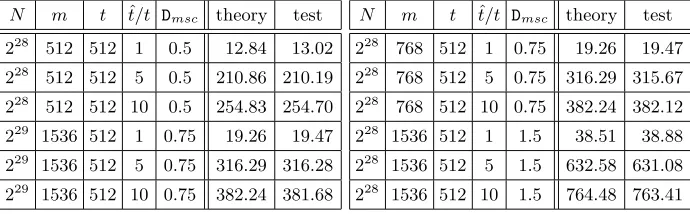
Table 1. Cost of resolving alarms when fully processing a single DP table with an online chain record
N m t t/tˆ Dmsc theory test
228
512 512 1 0.5 12.84 13.02
228
512 512 5 0.5 210.86 210.19
228
512 512 10 0.5 254.83 254.70
229
1536 512 1 0.75 19.26 19.47
229
1536 512 5 0.75 316.29 316.28
229
1536 512 10 0.75 382.24 381.68
N m t ˆt/t Dmsc theory test
228
768 512 1 0.75 19.26 19.47
228
768 512 5 0.75 316.29 315.67
228
768 512 10 0.75 382.24 382.12
228
1536 512 1 1.5 38.51 38.88
228
1536 512 5 1.5 632.58 631.08
228
1536 512 10 1.5 764.48 763.41
Experimental verification of (4) is summarized in Table 1. Each table entry corresponds to 2,000 randomly generated DP tables and 5,000 online chain cre-ations per table. All itercre-ations spent in dealing with alarms that were generated during this whole process were counted and divided by 2,000×5,000. The tests were conducted with different values of ˆtt andDmsc, so as to verify (4) at various
inputs. We also tried different m and t pairs that give the sameDmsc value to
verify that the formula is indeed a function of Dmsc. All the experiment results
are very close to our theory.
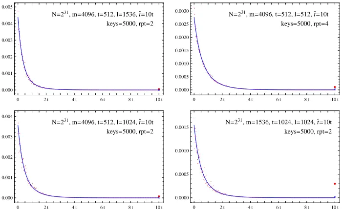
The second experiment validates our treatment of the parallel processing of tables. At the core of our associated argument is an equation obtained during the proof of Lemma 2, that expresses the probability for the processing of a table to stop at itsi-th iteration.4The theoretically obtained probability was compared
with values obtained through experiments. Working with the i-th termination probability, rather than Lemma 2, which gives the number of one-way function applications summed over alli, allows us more direct verification of finer details. After fixing various parameters, we first executed a complete pre-computation phase, thus preparing a set of ℓ tables. A simple XOR with a random fixed constant was used as the reduction function for each table. Then, we ran the pD online phase algorithm with a randomly generated inversion target and recorded the iteration count at which the processing of each table was terminated. The online phase was repeated with a certain number of random inversion targets. The process described so far, starting from the pre-computation phase to the multiple target inversions, was repeated a small number of times. Let us denote the number of inversion targets tried per pre-computation set by keys and the
4
number of complete pre-computation phases that were executed as rpt. The number of times each specific i was recorded, summed over all tables and test trials, was divided byℓ×keys×rpt, and was taken as the probability obtained through the experiment.
••
N=231, m=4096, t=512, l=1536, t`=10t
keys=5000, rpt=2
0 2 t 4 t 6 t 8 t 10 t
0.000 0.001 0.002 0.003 0.004 0.005
••
N=231, m=4096, t=512, l=512, t`=10t
keys=5000, rpt=4
0 2 t 4 t 6 t 8 t 10 t
0.0000 0.0005 0.0010 0.0015 0.0020 0.0025 0.0030
••
N=231, m=4096, t=512, l=1024, t`=10t
keys=5000, rpt=2
0 2 t 4 t 6 t 8 t 10 t
0.000 0.001 0.002 0.003 0.004
••
N=231, m=1536, t=1024, l=1024, t`=10t
keys=5000, rpt=2
0 2 t 4 t 6 t 8 t 10 t
0.0000 0.0005 0.0010 0.0015
Fig. 1.Probability for pD to stop processing of a specific table at the i-th iteration; Only approximately 240 out of the ˆt test values are plotted as dots in each graph (x-axis:i;y-axis: probability)
Test results are depicted as graphs in Figure 1. In each framed graph box, the tiny irregular (red) dots represent the experiment results and the smooth (blue) curve represents the theory. Because plotting all test results made the dots too densely packed and hard to see, we only plotted approximately 240 points among the ˆt points of each graph, with the intervals between plotted points shorter at smaller i values. The theoretic value for the i = ˆt position, which is expressed as a separate equation, is marked with an ×-sign and the corresponding experiment result is marked with a dot that is slightly larger than others. It is clear that the test results and theory are mostly in good agreement. However, the experiment data and theoretic value are visibly different at i= ˆt and this requires explanation.
The disagreement at i = ˆt is the largest for the right bottom graph. In this case the chain length bound ˆt = 10t = 10240 ≈ 213.3 is rather close to √
N = 215.5, and since such a choice does not satisfy the assumptions made in
not be an issue in practical applications of the tradeoff technique, whereNwould be much larger.
Let us discuss this matter slightly further. Recall that we had repeatedly used 1− 1
t
i
as the probability for a chain not to reach a DP until the i-th iteration. This value disregards the possibility of the chain looping back onto itself and a more exact expression is
i
Y
j=1
1−1t −Nj +
i
X
k=1
k N
k−1
Y
j=1
1−1t −Nj .
The value 1−1 t
i
is a good approximation of this, as long asi≪√N, but one knows from the birthday paradox that 1−1
t
i
will slowly deviate from the value given by the more complicated expression asiapproaches√N. We conducted a supplementary test, which we do not explain here due to page limits, to verify that our use of 1−1ti
as the ratio of non-DP chains remaining after the i-th iteration was indeed the cause of the discrepancy between theory and experiment ati= ˆt, when ˆtis close to √N.
6
Comparison of Tradeoff Algorithms
The analysis given in Section 4 contains enough information for us to make com-parisons between algorithms. We will first present a direct comparison between the pD and the original DP tradeoffs. Then, we will present the range of design options made available by the two DP variants and the rainbow tradeoffs com-pactly as graphs. These graphs will be of more practical value than the initial direct comparisons.
6.1 pD versus DP
As discussed in Section 3, the pD and the original DP tradeoffs will display identical coverage rate, require identical pre-computation cost, and succeed in recoveringxwith identical probability, when they are executed under the same set of parametersm,t, andℓ. The two algorithms also require the same amount of physical storage for DP tables and they only differ in the online execution time. Since the tradeoff coefficients are given as their respective T MN22 values, the online time complexities may directly be compared throughpDtcand Dtc. Here,
a smaller coefficient implies a more efficient tradeoff algorithm.
After reviewing the tradeoff coefficients as given by (3) and Theorem 1, one can see that they are expressed in a very similar form. In fact, the only dif-ference is in the first constant that sits inside the first set of parentheses. To compare the pD tradeoff against the original DP tradeoff, it suffices to evalu-ate ln(1−Dps)
Dps R1
0(1−Dps)
1−ulnu duat various success rates. Some explicit values
the corresponding constant of the original DP tradeoff, we have a sure indication that the pD tradeoff will outperform the original DP tradeoff.
We have clearly ranked pD over DP, but there is one issue that could affect this conclusion. The online memory access bottleneck of the pD tradeoff could remain a non-negligible overhead, even when the secondary DP technique men-tioned in Section 3 is applied, and one iteration of the pD tradeoff could take longer, on average, than that of the DP tradeoff. Should the circumstances be such that a marked difference in this iteration time is inevitable, the difference must be taken into account when interpreting a tradeoff coefficient ratio as a performance ratio. For example, if the pD tradeoff requires α time units per iteration and the DP tradeoff requiresβ time units per iteration, then one must compare the valuesα·pDtc and β·Dtc against each other rather than compare pDtcagainstDtc.
After seeing that pD outperforms DP, one naturally questions whether the improvement comes from the 6-th or the 7-th DP extension, i.e., whether keeping a record of the online chain or the parallel processing of tables was the main cause for the improvement. Let us refer to the DP variant that uses the first six of the seven DP extensions as the DP-OCR tradeoff. Details are not provided in this paper due to the page limit, but we have also analyzed DP-OCR in full. Results are that the tradeoff coefficient for DP-OCR falls between those of pD and DP, if all three are subject to the same parameters m, t, and ℓ. When parameters are such that only low inversion success rates (50%) are expected, DP-OCR performs quite close to pD, implying that the online chain record accounts for most of the improvement. However, when parameter achieving high success rates (99%) are chosen, DP-OCR stands approximately halfway between original DP and pD, implying that the parallelization does play a significant role in increasing efficiency.
6.2 pD versus Rainbow
Our next goal is to include the rainbow tradeoff in the comparison. This is not as straightforward as the comparisons between the two DP variants, mainly because of the large structural differences between the DP and rainbow tradeoffs. Below, we quickly review the approach of [11] before following it to present a fair comparison. The information required to draw the graphs for the rainbow tradeoff was also taken from [11]. NotationRpcandRtcwill be used to denote the
pre-computation coefficient and the tradeoff coefficient of the rainbow tradeoff, and the notationXpc andXtcwill be used when referencing the pre-computation
and tradeoff coefficients that are not specific to a tradeoff algorithm. The tradeoff coefficientXtc = T M
2
N2 is a measure of how efficiently the algo-rithm balances online time against storage requirements. A smallerXtcimplies a
more efficient tradeoff between online time and storage. However, better tradeoff efficiency usually requires a higher pre-computation cost and is not always de-sirable in practice. The optimal balance point between the tradeoff efficiencyXtc
and pre-computation costXpc is a subjective matter that cannot be arbitrarily
“tradeoff efficiency Xtc can be utilized, if pre-computation effort Xpc is
invested”
options that are made available by each algorithm, as a graph. Then, the imple-menter can make subjective decisions based on this compact display of possible choices and the physical resources that are available to him.
The above discussion would be sufficient for anyone interested in choosing pa-rameters for one fixed tradeoff algorithm. However, a little more care is required when comparing different algorithms. The range of possible options for each algo-rithm must be presented in a consistent manner. A common requirement on the success rate must be taken and the unit used to express the tradeoff coefficients must be unified. We have already seen that a direct comparison between pDtc
andDtcis justifiable. As for comparisons of these two against the rainbow
trade-off, let us simply state that pDtc and Dtc should be compared against 4Rtc (as
opposed toRtc) to be fair. The main reason is that, as discussed in Section 2, the
number of bits per table entry required by a rainbow tradeoff is roughly twice that of a DP tradeoff. The decision to comparepDtcagainst 4Rtcinvolves certain
assumptions, such as thatmandtare of similar order and that the bookkeeping of online chain records causes negligible overhead, but they are assumptions that are typically made during theoretic analysis of tradeoff algorithms and the de-tails should be clear to anyone with a full understanding of [11]. This concludes our short review of the approach to fair tradeoff comparison given by [11].
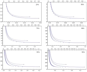
The range of (Xpc,Xtc) options each tradeoff algorithm is capable of providing
is given in Figure 2. To draw the graph, for example, corresponding to the DP tradeoff, one refers to (2) for the x-coordinate (pre-computation cost), substi-tutes (1) into (3) for the y-coordinate (tradeoff coefficient), and then plots the curve parameterized byDmsc.
In each framed graph box, the two curves and the sequence of dots should be seen as extending infinitely upwards. However, the right ends of the three graphs are either clearly marked or clearly visible. The curves start to go back up beyond the marked right ends, so that these marks correspond to the minimum tradeoff coefficient achievable by each algorithm. As going beyond this minimum implies using larger pre-computation while obtaining worse tradeoff efficiency, parameters corresponding to the parts that are not drawn should not be used.
We are now ready to discuss the implications of the graphs given in Figure 2. The graphs forDtcandpDtcare given by the dashed and solid lines, respectively.
The possible (Rpc,4Rtc) choices are given by the discrete sequence of dots. Each
dot corresponds to the use of a certain number of rainbow tables and since these table counts tend to be small, especially at low success rate requirements, the possible options appear spaced apart from each other. If one is required to fill in the space between the dots, one may extend horizontal lines to the right of each dot, until the line reaches over the dot to its right. Each box corresponds to a certain requirement on the probability of successful inversions.
25%
0.30 0.32 0.34 0.36 0.38 0.0
0.1 0.2 0.3 0.4 0.5
0 0.1 0.2 0.3 0.4 0.5 0.6 0.7 0.8
50%
0.70 0.75 0.80 0.85 0.90 0
1 2 3 4 5 6
0. 0.1 0.2 0.3 0.4 0.5 0.6 0.7 0.8
75%
1.4 1.5 1.6 1.7 1.8 0
5 10 15 20 25 30 35
0. 0.1 0.2 0.3 0.4 0.5 0.6 0.7 0.8 0.9
90%
2.4 2.6 2.8 3.0 3.2 0
20 40 60 80 100 120
0. 0.1 0.2 0.3 0.4 0.5 0.6 0.7 0.8 0.9 1.
95%
3.0 3.2 3.4 3.6 3.8 4.0 4.2 0
50 100 150 200
0. 0.1 0.2 0.3 0.4 0.5 0.6 0.7 0.8 0.9 1. 1.1
99%
5.0 5.5 6.0 6.5 0
100 200 300 400 500
0. 0.1 0.2 0.3 0.4 0.5 0.6 0.7 0.8 0.9 1. 1.1 1.2 1.3
Fig. 2.Tradeoff coefficients for the DP (dashed), pD (solid), and rainbow (large dots) tradeoffs in relation to pre-computation cost, at various success rates; Numeric values on each frame represent pre-computation iterations in units of N (bottom), tradeoff coefficient valuesDtc,pDtc, 4Rtc (left), and the matrix stopping constantsDmsc,pDmsc
that served as parameters for drawing the curves (top)
at a smaller pre-computation cost and that a better tradeoff efficiency can be obtained at equal pre-computation cost. Hence a very rough conclusion would be that the rainbow tradeoff is the best among the three algorithms.
Let us discuss this in more detail, starting with the case of success rate set to 25%. The optimal tradeoff coefficient reachable by the pD tradeoff ispDtc= 0.10. This tradeoff efficiency can be used if the available resources permit 0.376N it-erations of pre-computation. In comparison, the rainbow tradeoff achieves opti-mal tradeoff coefficient 4Rtc= 0.18 at 0.309N pre-computation iterations. Even
thoughpDtc = 0.10 and 4Rtc = 0.18 represent online time ratio of 1.8 at equal
However, another issue that is evident in the 25% case is that the rainbow tradeoff provides much less flexibility in options than the pD tradeoff. For ex-ample, the option of using pDtc = 0.11 atDpc = 0.336 is available with the pD
algorithm. Compared to the optimal efficiency of pDtc = 0.10 atDpc = 0.376,
this gives a valuable reduction in pre-computation cost at a small degradation of tradeoff efficiency. Unless the cost of pre-computation is extremely cheap, most implementers of the tradeoff algorithm will prefer to use pDtc = 0.11 over the optimal pDtc = 0.10. The rainbow tradeoff does not allow such a freedom of choice at the 25% probability of success.
Since the dots for the rainbow tradeoff are very close to the curve for the pD tradeoff, one can say that every option provided by the rainbow tradeoff can (nearly) be provided by the pD tradeoff. Since the pD tradeoff provides higher flexibility and even the possibility of a lower tradeoff coefficient, it seems safe to conclude that the pD tradeoff is preferable over the rainbow tradeoff at 25% success rate.
Even though we have explained at length that the pD tradeoff could be preferable over the rainbow tradeoff, the observations made for the 25% success rate are not very applicable to any of the other graph boxes. In the 50% success rate case, the optimal pD option of pDtc = 1.12 at Dpc = 0.915 is not a very
attractive choice over the rainbow option of 4Rtc = 1.17 at Rpc = 0.828, which
achieves similar tradeoff efficiency at a visibly lower pre-computation cost. Sim-ilarly, we havepDtc= 6.19 atDpc= 1.86 versus 4Rtc= 6.48 atRpc= 1.66 for the
75% success rate, andpDtc= 18.5 atDpc = 3.17 versus 4Rtc= 18.7 atRpc = 2.81
for the 90% success rate. At these moderate success rates, the minimum pDtc
is slightly better than the minimum 4Rtc, but its use cannot be justified when
pre-computation cost is taken into account. In fact, as discussed in the 25% suc-cess rate, implementers are likely to choose parameters somewhat away from the optimal tradeoff efficiency points, where the rainbow tradeoff is clearly advanta-geous over the pD tradeoff. As for higher success rates 95% and 99%, even the minimum 4Rtc is smaller than the minimumpDtc, so that there is no reason to
prefer the pD tradeoff over the rainbow tradeoff.
7
Conclusion
The parallel DP tradeoff studied in this work is a cryptanalytic time memory tradeoff algorithm that adds two extra techniques to the more widely known DP tradeoff. The first is to keep a full record of the online chain so that alarms can be resolved earlier during the pre-computation chain regeneration. The second idea is to process the multiple DP tables in parallel. This allows for more time to be spent in dealing with relatively shorter chains so that false alarms are hopefully reduced. We have confirmed that both of these ideas have positive effects on the efficiency of the DP tradeoff.
tradeoffs. The comparison of tradeoff efficiency was done in a fair manner in the sense that factors such as the success probability of inversion, the storage size in number of bits, and pre-computation cost were all taken into account. Hence, the comparison results have practical implications on the choice of which tradeoff algorithm to use.
Comparisons show that, even with the extra enhancements, the pD tradeoff is not likely to be preferable over the rainbow tradeoff under most situations. The only exception is when the success rate requirement is very low. For ex-ample, when dealing with multi-target time memory tradeoffs [5], where the rainbow tradeoff is known to be much less efficient than both the original Hell-man and DP tradeoffs, our analysis is an indication that the use of the pD tradeoff could be advantageous over the original DP tradeoff. At moderate suc-cess rate requirements, the pD tradeoff can be slightly more efficient than the rainbow tradeoff, but the choice to use the pD tradeoff cannot be justified when the pre-computation cost is taken into account.
In short, when reduction in wall-clock running time is very important and one is willing to parallelize the online phase to a very high degree, depending on the degree of parallelization available, variants of the DP tradeoff could be a reasonable choice. However, if total CPU time is more important than wall-clock time, one should work with the rainbow tradeoff. Still, the pD tradeoff is more efficient than the usual DP tradeoff, in that it requires a smaller total number of function iterations, when the two are provided with the same pre-computation table.
The theoretic analysis and the resulting concrete graphs of this paper can easily be adjusted to cope with various specific situations and allow for educated decisions. For example, when run on resource constrained environments such as GPUs, iterations of pD may take longer than those of DP due to pD’s higher demands for online memory. In this situation, it suffices to scale the tradeoff coefficients of pD and DP according to their respective average iteration timings before comparing their graphs to conclude whether the online memory require-ment undermines the small advantage of pD over DP.
References
1. G. Avoine, P. Junod, P. Oechslin, Characterization and improvement of time-memory trade-off based on perfect tables.ACM Trans. Inform. Syst. Secur.,11(4), 17:1–17:22 (2008). Preliminary version presented at INDOCRYPT 2005.
2. J. Borst,Block Ciphers: Design, Analysis, and Side-Channel Analysis. Ph.D. The-sis, Katholieke Universiteit Leuven, September 2001
3. J. Borst, B. Preneel, J. Vandewalle, On the time-memory tradeoff betweeen exhaus-tive key search and table precomputation. InProceedings of the 19th Symposium on Information Theory in the Benelux, WIC, 1998
5. A. Biryukov, A. Shamir, Cryptanalytic time/memory/data tradeoffs for stream ci-phers, InAdvances in Cryptology—ASIACRYPT 2000. LNCS, vol. 1976, (Springer, 2000), pp. 1–13.
6. A. Biryukov, A. Shamir, D. Wagner, Real time cryptanalysis of A5/1 on a PC. In
FSE 2000, LNCS1978, (Springer, 2001), pp. 1–18
7. D. E. Denning,Cryptography and Data Security (Addison-Wesley, 1982)
8. M. E. Hellman, A cryptanalytic time-memory trade-off. IEEE Trans. on Infor. Theory,26, (1980), pp. 401–406.
9. Y. Z. Hoch, Security analysis of generic iterated hash functions. Ph.D. Thesis, Weizmann Institute of Science, August 2009.
10. J. Hong,Des. Codes Cryptogr., The cost of false alarms in Hellman and rainbow tradeoffs.57(3), (Springer, 2010), pp.293–327.
11. J. Hong, S. Moon, A comparison of cryptanalytic tradeoff algorithms. Cryptology ePrint Archive. Report 2010/176.
12. A. Narayanan, V. Shmatikov, Fast dictionary attacks on passwords using time-space tradeoff.Proceedings of the 12th ACM CCS. (ACM, 2005), pp. 364–372. 13. P. Oechslin, Making a faster cryptanalytic time-memory trade-off. inAdvances in
Cryptology–CRYPTO 2003, LNCS, vol. 2729, (Springer, 2003) pp .617–630. 14. A. Shamir, Random Graphs in Security and Privacy. Invited talk at ICITS 2009. 15. F.-X. Standaert, G. Rouvroy, J.-J. Quisquater, J.-D. Legat, A time-memory
trade-off using distinguished points: New analysis & FPGA results. In Cryptographic Hardware and Embedded Systems—CHES 2002, LNCS 2523, (Springer, 2003), pp. 593–609
A
Technical Proofs of Lemmas
Full proofs to the three lemmas that were introduced in Section 4 are provided here. The proofs mostly consist of careful applications of the random function arguments followed by some technical computations.
A.1 Lemma 1
We want to compute the number ←
mi of distinct points situated at distance i
from the ending points in a DP matrix.
Consider a DP matrix constructed with a sufficiently largeˆtt. We may assume
that the fraction of wasted pre-computation iterations ˆtt 1−1 t
ˆt
≈ ˆt texp(−
ˆ t t) is
very small. This implies that only a negligible fraction of the points on which the random function F was defined is discarded during the pre-computation table creation.
Let us fix a specific method for counting the number of distinct non-ending points in the DP matrix. These points are the inputs on which the random function images were defined and their total number is expected to be Dcrmt.
could also count by columns or choose a more complicated walk through the DP matrix.
Regardless of the counting method that is taken, one can view the points that are counted as those inputs on which the random function was randomly defined without any restriction. Chain iterations computed on all otherF-input points of the DP matrix can be seen as having followed the random function definitions made on the counted points.
Since theF-image definitions were made randomly on theDcrmtfresh points,
we can expectDcrmt1t many of these points to have been mapped to DPs byF.
The discussion at the beginning parts of this proof assures us that the ratio 1t of points mapped to DPs has not been altered inadvertently by the discarded pre-computation. These points that were mapped to DPs are clearly the points situated one iteration away from the DP ending points and these contain no duplicates. A straightforward extension of this idea is that Dcrmt 1− 1t)i−1 1t
many distinct points are found iiterations away from the DPs, as claimed.
A.2 Lemma 2
The cost of creating the online chain is given by this lemma. Even though pD processes allℓtables in parallel, let us focus on a single fixed table and compute the expected work associated with its processing. The total cost will then be ℓ times the value we compute.
The initial searching of the inversion targety=F(x) among the DPs, which requires no F invocation, will be referred to as the 1-st iteration. As explained at the end of Section 3, we take the convention that the outcome from the i-th iteration of one table does not affect the i-th iteration of another table. Only strictly previous iterations will have the possibility of affecting the current iteration.
The pD algorithm will terminate the online chain creation for the table under our focus right after processing thei-th iterations for all tables if and only if one of the following events occur.
1. The online chain for the table under focus became a DP chain of length5 i, while none of the other ℓ−1 tables produced the correct answer x to be recovered up to thei-th iteration.
2. The online chain for the table under focus did not reach a DP up to thei-th iteration, and the correctx was found for the first time in one (or more) of the otherℓ−1 tables at thei-th iteration.
3. The online chain for the table under focus became a DP chain of length i, and the correct inversexwas found for the first time in one (or more) of the otherℓ−1 tables at thei-th iteration.
5
Note that the above three events are mutually exclusive and that the two sub-events that constitute each of the above three sub-events are independent from each other.
Let us compute the probability for the first event to occur. The online chain requirement is satisfied with probability 1−1
t
i−1 1
t. As for the inversion failure
part, observe that no two distinct columns of a DP matrix, aligned at its ending points, can contain a common element. Hence the number of distinct points, used as inputs toF during table creation, that lie within iiterations away from the ending points, is given byPi
j=1
←
mj. The probability for the other tables to fail in
producing the correct inverse up until thei-th iteration is thus 1− Pi
j=1
←
mj
N
ℓ−1
. The second event is discussed next. Its online chain part occurs with prob-ability 1−1
t
i
. As for the part concerning the recovery of x, one must suc-ceed in recovering the inverse within the first i iterations, but not succeed within the first i−1 iterations. This probability is given by the difference
1− 1 −
Pi j=1
←
mj
N
ℓ−1
−
1− 1−
Pi−1 j=1
←
mj
N
ℓ−1
. We emphasize that suc-cessful inversion before thei-th iteration must be ruled out, so that the simpler expression 1− 1−←mi
N
ℓ−1
does not serve our need.
After the probability for the third event is similarly computed, we can write the probability for the processing of the table under focus to stop at the i-th iteration to be
1−1
t i−11
t 1− Pi j=1 ← mj N
ℓ−1
+1−1 t
in 1−
Pi−1
j=1
←
mj
N
ℓ−1
−1−
Pi
j=1
←
mj
N
ℓ−1o
+1−1 t
i−11
t n
1− Pi−1
j=1
←
mj
N
ℓ−1
−1−
Pi
j=1
←
mj
N
ℓ−1o .
If we apply Lemma 1, the approximation (1−1/a)b
≈e−b/a, andD
pc =mtℓN , we
arrive at
1−1t
i−1
exp−DpcDcr
n
1−1−1t i−1o
−1−1 t
i
exp−DpcDcr
n
1−1−1 t
io ,
(5)
which is correct for 1≤i <ˆt. In order for all the probabilities to add up to 1, the final probability ati= ˆtshould clearly be
1−1
t ˆt−1
exp−DpcDcr
n
1−1−1 t
ˆt−1o
Since stopping at thei-th iteration impliesi−1 iterations ofF, the cost of online chain creation for the single table under our focus can be written as
n
ˆ t−1
X
i=1
Equation (5)
·(i−1)o+ Equation (6)
·(ˆt−1)
=
ˆ t−1
X
i=1
1−1t
i
exp−DpcDcr
n
1−1−1t io
≈t Z t/tˆ
0
e−x exp −D
pcDcr 1−e−xdx.
One can compute this explicitly and find it to be
t
DpcDcr
1−exp −DpcDcr(1−e−ˆt/t)
≈ t
DpcDcr
1−exp(−DpcDcr) =
t
DpcDcr Dps,
where the approximation is valid for sufficiently large tˆ
t. To arrive at the formula
claimed by Lemma 2, it now suffices to multiplyℓ to the above and then apply
1 ℓDpc=
1 tpDmsc.
A.3 Lemma 3
The number of one-way function iterations required to resolve alarms is given by this lemma. We will continue to use the convention that was explained in the previous subsection concerning the labeling of iterations and how only strictly previous iterations can affect the current iteration. As before, we focus our at-tention on a single table.
Let us assume that thei-th iteration of the online chain for this table resulted in a DP and compute the work expected to deal with the alarm which may or may not result from this DP. Even though the pre-computation chains were generated long before the current online chain, we treat each pre-computation chain as if it were being freshly generated and study how it might collide with the current online DP chain of lengthi. That is, we generate a pre-computation chain with a random function that has only been defined on the online chain so far.
The probability for a randomly created chain to collide with a given online chain of lengthiat thej-th iteration is
1−1
t − i N
j−1i+ 1
N ≈exp − j t
i+ 1 N .
of the (i+ 1) online chain points. The approximation ignores the i
N term, since
it is of much smaller order than 1 t.
Note that the length of a pre-computation chain is at most ˆt. This implies that, as the j values approach ˆt, we know beforehand that the next iteration images will not land on the online chain points that are far from the ending point. More precisely, we can write the probability for a random pre-computation chain to collide with the online chain at distance j ≤ˆt from the starting point of the pre-computation chain as
j−2
Y
k=0
1−1t − min{i+ 1,ˆt−k}
N−(i+ 1−min{i+ 1,ˆt−k})
× min{i+ 1,ˆt−j+ 1}
N−(i+ 1−min{i+ 1,ˆt−j+ 1})
≈exp−jtmin{i+ 1,Ntˆ−j+ 1}.
Since pD keeps a record of the complete online chain (the 6-th extension to DP), if the online chain merges with the pre-computation chain at distance j from the starting point of the computation chain, regeneration of the pre-computation to resolve alarms can be stopped at thej-th iteration. Also recall that the regeneration of a pre-computation chain need not exceed (ˆt−i+ 1) iterations (the 5-th extension to DP). The expected cost of resolving alarms which may or may not occur from an online DP chain of lengthican be written as
ˆ t
X
j=1
min{j,ˆt−i+ 1} m
1−e−ˆt/t
exp−jtmin{i+ 1,Ntˆ−j+ 1}
≈ m
1−e−ˆt/t
t3 N
Z t/tˆ
0
minnx,ˆt t −
i t
o
exp(−x) minni t,
ˆ t t−x
o dx
= Dmsc 1−e−ˆt/t
tni t 1−e
−ˆt/t−ˆt
t e
i/t −1
e−ˆt/t
o
. (7)
We are finally ready to write down the cost of dealing with alarms. It suffices to combine the above expected work with the probability for other tables not to produce the correct answer up to the (i−1)-st iteration and the probability for the online chain we are focusing on to become a DP chain of lengthi. Recalling that the cost must be added over all ℓ tables, the cost of dealing with alarms can be written as
ℓ ˆ t X i=1 1−
Pi−1
j=1
←
mj
N
ℓ−1
·1−1t i−11
t·
Dmsc
1−e−ˆt/tt
ni t 1−e
−ˆt/t−ˆt
t e
i/t −1
e−t/tˆ
After using Lemma 1 to replace thePi−1
j=1
←
mj, this can be approximated by the
integral expression
Dmscℓt
Z ˆt/t
0
exp −DpcDcr(1−e−x)e−x
x−ˆtt e x
−1
eˆt/t−1
dx.
By applying change of variables to the first termDmscℓt R ˆ t/t
0 exp −DpcDcr(1−
e−x)e−xx dx of this expression, we can rewrite it as
−Dmscℓt
Z 1
e−t/tˆ
exp −DpcDcr(1−u)(−lnu) (−du).
The formula stated in the lemma is a tweaked version of this equation that can be obtained by applying the relations Dmscl = Dpct, Dps = 1−e−DpcDcr, and
e−ˆt/t≈0.
It only remains to deal with the second term. One can easily check that
0 ≤Dmscℓt
Z ˆt/t
0
exp −DpcDcr(1−e−x)e−x
ˆt t
ex−1 eˆt/t−1
dx
= Dmscℓt
ˆ t/t eˆt/t−1
Z ˆt/t
0
1−e−x
exp DpcDcr(1−e−x)dx ≤
Dmscℓt
(ˆt/t)2
eˆt/t−1,