Joppe W. Bos1
, Thorsten Kleinjung1
, Ruben Niederhagen2,3
, and Peter Schwabe3 ⋆
1
Laboratory for Cryptologic Algorithms EPFL, Station 14, CH-1015 Lausanne, Switzerland
{joppe.bos, thorsten.kleinjung}@epfl.ch
2 Department of Electrical Engineering
National Taiwan University, 1 Section 4 Roosevelt Road, Taipei 106-70, Taiwan [email protected]
3
Department of Mathematics and Computer Science
Technische Universiteit Eindhoven, P.O. Box 513, 5600 MB Eindhoven, Netherlands [email protected]
Abstract. This paper describes an implementation of Pollard’s rho algorithm to compute the elliptic curve discrete logarithm for the Synergistic Processor Elements of the Cell Broadband Engine Architecture. Our implementation targets the elliptic curve discrete logarithm problem defined in the Certicom ECC2K-130 challenge. We compare a bitsliced implementation to a non-bitsliced implementation and describe several optimization techniques for both approaches. In particular, we address the question whether normal-basis or polynomial-basis representation of field elements leads to better performance. Using our software, the ECC2K-130 challenge can be solved in one year using the Synergistic Processor Units of less than 2700 Sony Playstation 3 gaming consoles.
Keywords: Cell Broadband Engine Architecture, elliptic curve discrete logarithm problem, binary-field arithmetic, parallel Pollard rho
1 Introduction
How long does it take to solve the elliptic curve discrete logarithm problem (ECDLP) on a given elliptic curve using given hardware? This question was addressed recently for the Koblitz curve defined in the Certicom challenge ECC2K-130 for a variety of hardware platforms [2] This paper zooms into Section 6 of [2] and describes the implementation of the parallel Pollard rho algorithm [19] for the Synergistic Processor Elements of the Cell Broadband Engine Architecture (CBEA) in detail. We discuss our choice to use the technique of bitslicing [7] to accelerate the underlying binary-field arithmetic operations by comparing a bitsliced to a non-bitsliced implementation.
Many optimization techniques for the non-bitsliced version do not require independent parallel computations (batching) and are therefore not only relevant in the context of crypt-analytical applications but can also be used to accelerate cryptographic schemes in practice. To the best of our knowledge this is the first work to describe an implementation of high-speed binary-field arithmetic for the CBEA. We plan to put all code described in this paper into the public domain to maximize reusability of our results.
Related work. The work closest to ours is [9] in which Bos, Kaihara, and Montgomery describe an implementation of Pollard’s rho algorithm for the CBEA to solve an 112-bit prime ECDLP. A brief comparison with their results is given in Section 7.
⋆
Organization of the paper. In Section 2 we describe the features of the CBEA which are relevant to this paper. To make this paper self contained we briefly recall the parallel version of Pollard’s rho algorithm and summarize the choice of the iteration function in Section 3. Section 4 discusses different approaches to a high-speed implementation of the iteration function on the CBEA. In Sections 5 and 6 we describe the non-bitsliced and the bitsliced implementation, respectively. We compare our results to previous work and conclude the paper in Section 7.
2 A Brief Description of the Cell processor
The Cell Broadband Engine Architecture [14] was jointly developed by Sony, Toshiba and IBM. Currently, there are two implementations of this architecture, the Cell Broadband En-gine (Cell/B.E.) and the PowerXCell 8i. The PowerXCell 8i is a derivative of the Cell/B.E. and offers enhanced double-precision floating-point capabilities and a different memory inter-face. Both implementations consist of a central Power Processor Element (PPE), based on the Power 5 architecture and 8 Synergistic Processor Elements (SPEs) which are optimized for high-throughput vector instructions. All units are linked by a high-bandwidth (204 GB/s) ring bus.
The Cell/B.E. can be found in the IBM blade servers of the QS20 and QS21 series, in the Sony Playstation 3, and several acceleration cards like the Cell Accelerator Board from Mercury Computer Systems. The PowerXCell 8i can be found in the IBM QS22 servers. Note that the Playstation 3 only makes 6 SPEs available to the programmer.
The code described in this paper runs on the SPEs directly and does not interact with the PPE or other SPEs during core computation. We do not take advantage of the extended capabilities of the PowerXCell 8i. In the remainder of this section we will describe only those features of the SPE which are of interest for our implementation and are common to both the Cell/B.E. and the PowerXCell 8i. Therefore we may address the Cell/B.E. and the PowerXCell 8i jointly as theCell processor orCell CPU. Further information on the current implementations of the Cell Broadband Engine Architecture can be found in [16].
Each SPE consists of a Synergistic Processor Unit (SPU) as its computation unit and a
Memory Flow Controller(MFC) which grants access to the ring bus and therefore in particular to main memory.
2.1 SPU – architecture and instruction set
The SPU is composed of three parts: TheSynergistic Execution Unit (SXU) is the computa-tional core of each SPE. It is fed with data either by the SPU Register File Unit (RFU) or by the Local Storage (LS) that also feeds the instructions into the SXU.
The RFU contains 128 general purpose registers with a width of 128 bits each. The SXU has fast and direct access to the LS but the LS is limited to only 256 KB. The SXU does not have transparent access to main memory; all data must be transferred from main memory to LS and vice versa explicitly by instructing the DMA controller of the MFC. Due to the relatively small size of the LS and the lack of transparent access to main memory, the programmer has to ensure that instructions and the active data set fit into the LS and are transferred between main memory and LS accordingly.
even pipeline, which execute disjoint subsets of the instruction set. The even pipeline handles floating point operations, integer arithmetic, logical instructions, and word SIMD shifts and rotates. The odd pipeline executes byte-granularity shift, rotate-mask, and shuffle operations on quadwords, and branches as well as loads and stores.
Up to two instructions can be issued each cycle, one in each pipeline, given that alignment rules are respected (i.e., the instruction for the even pipeline is aligned to a multiple of 8 bytes and the instruction for the odd pipeline is aligned to a multiple of 8 bytes plus an offset of 4 bytes), that there are no interdependencies to pending previous instructions for either of the two instructions, and that there are in fact at least two instructions available for execution. Therefore, a careful scheduling and alignment of instructions is necessary to achieve peak performance.
2.2 MFC – accessing main memory
As mentioned before, the MFC is the gate for the SPU to reach main memory as well as other processor elements. Memory transfer is initiated by the SPU and afterwards executed by the DMA controller of the MFC in parallel to ongoing instruction execution by the SPU.
Since data transfers are executed in background by the DMA controller, the SPU needs feedback about when a previously initiated transfer has finished. Therefore, each transfer is tagged with one of 32 tags. Later on, the SPU can probe either in a blocking or non-blocking way if a subset of tags has any outstanding transactions. The programmer should avoid to read data buffers for incoming data or to write to buffers for outgoing data before checking the state of the corresponding tag to ensure deterministic program behaviour.
2.3 LS – accessing local storage
The LS is single ported and has a line interface of 128 bytes width for DMA transfers and instruction fetch as well as a quadword interface of 16 bytes width for SPU load and store. Since there is only one port, the access to the LS is arbitrated using the following priorities:
1. DMA transfers (at most every 8 cycles) 2. SPU load/store
3. instruction fetch
Instructions are fetched in lines of 128 bytes, i.e., 32 instructions. In the case that all instructions can be dual issued, new instructions need to be fetched every 16 cycles. Since SPU loads/stores have precedence over instruction fetch, in case of high memory access there should be an lnopinstruction for the odd pipeline every 16 cycles to avoid instruction starvation. If there are ongoing DMA transfers an hbrpinstruction should be used giving instruction fetch explicit precedence over DMA transfers.
2.4 Determining performance
The CBEA offers two ways to determine performance of SPU code: performance can either be statically analysed or measured during runtime.
analysis. The “IBM SDK for Multicore Acceleration” [15] contains the toolspu timingwhich performs this static analysis and gives quite accurate cycle counts.
This tool has the disadvantage that it assumes fully linear execution and does not model instruction fetch. Therefore the results reported byspu timingare overly optimistic for code that contains loops or a high number memory of accesses. Furthermore,spu timingcan only be used inside a function. Function calls—in particular calling overhead on the caller side—can not be analysed.
Measurement during runtime.Another way to determine performance is through an in-tegrated decrementer (see [16, Sec. 13.3.3]). Measuring cycles while running the code captures all effects on performance in contrast to static code analysis.
The disadvantage of the decrementer is that it is updated with the frequency of the so-called timebase of the processor. The timebase is usually much smaller than the processor frequency. The Cell/B.E. in the Playstation 3 (rev. 5.1) for example changes the decrementer only every 40 cycles, the Cell/B.E. in the QS21 blades even only every 120 cycles. Small sections of code can thus only be measured on average by running the code several times repeatedly.
For cycle counts we report in this paper we will always state whether the count was obtained usingspu timing, or measured by running the code.
3 Preliminaries
The main task on solving the Certicom challenge ECC2K-130 is to compute a specific discrete logarithm on a given elliptic curve. Up to now, the most efficient algorithm known to solve this challenge is a parallel version of Pollard’s rho algorithm running concurrently on a big number of machines.
In this section we give the mathematical and algorithmic background necessary to under-stand the implementations described in this paper. We will briefly explain the parallel version of Pollard’s rho algorithm, review the choice of the iteration function described in [2], and introduce the framework of our implementation.
3.1 The ECDLP and parallel Pollard rho
The security of elliptic-curve cryptography relies on the believed hardness of the elliptic curve discrete logarithm problem (ECDLP): Given an elliptic curve E over a finite fieldFqand two pointsP ∈E(Fq) andQ∈ hPi, find an integerk, such thatQ= [k]P. Here, [k] denotes scalar multiplication with k.
If the order of hPi is prime, the best-known algorithm to solve this problem (for most elliptic curves) is Pollard’s rho algorithm [19]. In the following we describe the parallelized collision search as implemented in [2]. See [2] for credits and further discussion.
The algorithm uses a pseudo-random iteration function f : hPi → hPi and declares a subset of hPi as distinguished points. The parallelization is implemented in a client-server approach in which each client node generates an input point with known linear combination in P and Q, i.e. R0 = [a0]P + [b0]Q with a0 and b0 generated from a random seed s. It
The server searches for a collision in all distinguished points sent by the clients, i.e. two different input points reaching the same distinguished point Rd. The iteration function is constructed in such a way that the server can computead andbd such thatRd=adP+bdQ from a0 and b0 (which are derived from s). If two different input points yield a collision
at a distinguished point Rd, the server computes the two (most probably different) linear combinations of the pointRd inP and Q:Rd= [ad]P + [bd]Q and Rd = [cd]P + [dd]Q. The solution to the discrete logarithm ofQto the base P is then
Q=
ad−cd bd−dd
P.
The expected number of distinguished points required to find a collision depends on the density of distinguished points in hPi. The expected amount of iterations of f on all nodes in total is approximately
q
π|hPi|
2 assuming the iteration function f is a random mapping of
size |hPi| (see [13]).
3.2 ECC2K-130 and our choice of the iteration function
The specific ECDLP addressed in this paper is given in the Certicom challenge list [10] as challenge ECC2K-130. The given elliptic curve is a Koblitz curve E :y2
+xy =x3
+ 1 over the finite field F2131; the two given points P and Q have orderl, where l is a 129-bit prime.
The challenge is to find an integer ksuch that Q= [k]P. In the following we will describe the choice of the iteration function used in [2]. For a more detailed description please refer to [2], for a discussion and comparison to other possible iteration functions also see [1].
Given a point (x, y) on the curve it is computationally easy to determine its negative (x, x+ y). A common optimization technique for Pollard’s rho algorithm is to work on equivalence classes modulo negation of points. This reduces the expected number of iterations by a factor of up to√2 [22,11], but it requires the iteration function to be well-defined on equivalence classes modulo negation.
For Koblitz curves a generalization of this idea can be used to reduce the expected number of iterations even further: As the curve equation has coefficients in F2, the i-th powers of
the Frobenius endomorphism σi : E(F
2131) → E(F2131),(x, y) 7→ (x2
i
, y2i), i = 1, . . .130 are
efficiently computable automorphisms besides negation. We can thus reduce the number of iterations by a total factor of up to √2·131 by considering orbits under the 131 i-th power Frobenius endomorphisms and negation.
We define a pointRi (representing an equivalence class) as distinguished if the Hamming weight, i.e. the number of bits set, of thex-coordinate in normal basis representation HW(xRi) is smaller than or equal to 34. Observe that this property respects the orbits of negation (because the x-coordinate remains the same) and of the Frobenius endomorphism (because squaring in normal basis is just a cyclic rotation of bits, not affecting the Hamming weight).
The iteration function is defined as
Ri+1 =f(Ri) =σj(Ri) +Ri,
where j = ((HW(xRi)/2)mod 8) + 3. The iteration function is well-defined on equivalence classes modulo negation and application of σ, because both are endomorphisms.
a collision has been detected, it is possible to recompute the two according iterations and update the coefficientsai and bifollowing this rule. This gives the coefficients to compute the discrete logarithm.
3.3 Computing the iteration function
Computing the iteration function requires one application of σj and one elliptic-curve addi-tion. Furthermore we need to convert thex-coordinate of the resulting point to normal basis, if a polynomial-basis representation is used, and check whether it is a distinguished point.
Many applications use so-called inversion-free coordinate systems to represent points on elliptic curves (see, e.g., [12, Sec. 3.2]) to speed up the computation of point multiplications. These coordinate systems use a redundant representation for points. Identifying distinguished points requires a unique representation, this is why we use the affine Weierstrass represen-tation to represent points on the elliptic curve. Elliptic-curve addition in affine Weierstrass coordinates on the given elliptic curve requires 2 multiplications, one squaring, 6 additions, and 1 inversion in F2131 (see, e.g. [6]). Application of σj means computing the 2j-th powers
of the x- and the y-coordinate. In total, one iteration takes 2 multiplications, 1 squaring, 2 computations of the form r2m
, with 3 ≤ m ≤10, 1 inversion, 1 conversion to normal-basis, and one Hamming-weight computation. In the following we will refer to computations of the formr2m
asm-squaring.
A note on the inversion.To speed up the relatively costly inversion we can batch several inversions and use Montgomery’s trick [18]: m batched inversions can be computed with 3(m −1) multiplications and one inversion. For example, m = 64 batched elliptic curve additions take 2·64 + 3·(64−1) = 317 multiplications, 64 squarings and 1 inversion. This corresponds to 4.953 multiplications, 1 squaring and 0.016 inversions for a single elliptic-curve addition.
4 Approaches for implementing the iteration function
In the following we discuss the two main design decisions for the implementation of the iteration function: 1.) Is it faster to use bitslicing or a standard approach and 2.) is it better to use normal-basis or polynomial-basis representation for elements of the finite field.
4.1 Bitsliced or not bitsliced?
Binary-field arithmetic was commonly believed to be more efficient than prime-field arith-metic for hardware but less efficient for software implementations. This is due to the fact that most common microprocessors spend high effort on accelerating integer- and floating-point multiplications. Prime-field arithmetic can benefit from those high-speed multiplication algo-rithms, binary-field arithmetic cannot. However, Bernstein showed recently that for batched
multiplications, binary fields can provide better performance than prime fields also in software [3]. In his implementation of batched Edwards-curve arithmetic the bitslicing technique [7] is used to compute (at least) 128 binary-field multiplications in parallel on an Intel Core 2 processor.
131 coefficients of an element, one register per bit. Algorithms are then implemented by simulating a hardware implementation – gates become bit operations such as AND and XOR. For one element in 131 registers this is highly inefficient, it may become efficient if all 128 bits of the registers are used for 128 independent (batched) operations. The lack of registers—most architectures including the SPU do not support 131 registers—can easily be compensated for by spills, i.e. storing currently unused values on the stack and loading them when they are required.
The results of [3] show that for batched binary-field arithmetic on the Intel Core 2 pro-cessor bitsliced implementations are faster than non-bitsliced implementations. However, the question whether this is also the case on the SPU of the Cell processor is hard to answer a priori for several reasons:
– The Intel Core 2 can issue up to 3 bit operations on 128-bit registers per cycle, an obvious lower bound on the cycles per iteration is thus given as the number of bit operations per cycle divided by 3. The SPU can issue only one bit operation per cycle, the lower bound on the performance is thus three times as high.
– Bernstein in [3, Sec. 3] describes that the critical bottleneck for batched multiplications are in fact loads instead of bit operations. The Core 2 has only 16 architectural 128-bit registers and can do only 1 load per cycle, i.e. one load per 3 bit operations.
The SPUs have 128 architectural 128-bit registers and can do one load per bit operation. However, unlike on the Core 2, the load operations have to compete with store operations. Due to the higher number of registers and the lower arithmetic/load ratio it seems easier to come close to the lower bound of cycles imposed by the number of bit operations on the SPUs than on the Core 2. How much easier and how close exactly was very hard to foresee a priori.
– Bitsliced operations rely heavily on parallelism and therefore require much more storage for inputs, outputs and intermediate values. As described in Section 2, all data of the active set of variables has to fit into 256 KB of storage alongside the code. In order to make code run fast on the SPU which executes all instructions in order, optimization techniques such as loop unrolling and function inlining are crucial; these techniques increase the code size and make it harder to fit all data into the local storage.
– Montgomery inversions require another level of parallelism, inverting for example 64 val-ues in parallel requires 64·128 field elements (131 KB) of inputs when using bitsliced representation. This amount of data can only be handled using DMA transfers between the main memory and the local storage. In order to not suffer from performance penalties due to these transfers, they have to be carefully interleaved with computations.
We decided to evaluate which approach is best by implementing both, the bitsliced and the non-bitsliced version, independently by two groups in a friendly competition.
4.2 Polynomial or normal basis?
Another choice to make for both bitsliced and non-bitsliced implementations is the repre-sentation of elements ofF2131: Polynomial bases are of the form (1, z, z2, z3, . . . , z130), so the
basis elements are increasing powers of some elementz∈F2131. Normal bases are of the form
(α, α2, α4, . . . , α2130), so each basis element is the square of the previous one.
before computing the Hamming weight in normal basis. On the other hand, implementations of multiplications in normal basis are widely believed to be much less efficient than those of multiplications in polynomial basis.
In [21], von zur Gathen, Shokrollahi and Shokrollahi proposed an efficient method to multiply elements in type-2 normal basis representation. Here we review the multiplier shown in [2]; see [2] for further discussion and history:
An element of F2131 in type-2 normal basis representation is of the form
f0(ζ+ζ−1) +f1(ζ2+ζ−2) +f2(ζ4+ζ−4) +· · ·+f130(ζ2 130
+ζ−2130
),
where ζ is a 263rd root of unity in F2131. This representation is first permuted to obtain
coefficients of
ζ+ζ−1
, ζ2
+ζ−2
, ζ3
+ζ−3
, . . . , ζ131
+ζ−131
,
and then transformed to coefficients in polynomial basis ζ+ζ−1
,(ζ+ζ−1
)2
,(ζ+ζ−1
)3
, . . . ,(ζ+ζ−1
)131
.
Applying this transform to both inputs allows us to use a fast polynomial-basis multiplier to retrieve coefficients of
(ζ+ζ−1)2,(ζ+ζ−1)3, . . . ,(ζ +ζ−1)262. Applying the inverse of the input transformation yields coefficients of
ζ2+ζ−2, ζ3+ζ−3, . . . , ζ262+ζ−262.
Conversion to permuted normal basis just requires adding appropriate coefficients, for example ζ200
is the same asζ−63
and thusζ200
+ζ−200
is the same asζ63
+ζ−63
. To obtain the normal-basis representation we only have to apply the inverse of the input permutation.
This multiplication still incurs overhead compared to modular multiplication in polynomial basis, but it needs careful analysis to understand whether this overhead is compensated for by the above-described benefits of normal-basis representation. Observe that all permutations involved in this method are free for hardware and bitsliced implementations while they are quite expensive in non-bitsliced software implementations.
5 The non-bitsliced implementation
For the non-bitsliced implementation, we decided not to implement arithmetic in a normal-basis representation. The main reason is that the required permutations, splitting and revers-ing of the bits, as required for the conversions in the Shokrollahi multiplication algorithm (see Section 4.2) are too expensive to outweigh the gain of having no basis change and faster m-squarings.
The non-bitsliced implementation uses a polynomial-basis representation of elements in F2131 ∼=F2[z]/(z131+z13+z2+z+ 1). Field elements in this basis can be represented using
Algorithm 1The reduction algorithm for the ECC2K-130 challenge used in the non-bitsliced version. The algorithm is optimized for 128-bit architectures.
Input: C=A·B=a+b·z128
+c·z256
, such thatA, B∈F2[z]/(z 131
+z13
+z2
+z+ 1) anda, b, care 128-bit strings representing polynomial values.
Output: D=Cmod (z131
+z13
+z2
+z+ 1). 1: c←(c≪109) + (b≫19)
2: b←bAND(219 −1)
3: c←c+ (c≪1) + (c≪2) + (c≪13) 4: a←a+ (c≪16)
5: b←b+ (c≫112) 6: x←(b≫3) 7: b←bAND7
8: a←a+x+ (x≪1) + (x≪2) + (x≪13) 9: return(D=a+b·z128
)
The implementation of an addition is trivial and requires two XOR instructions. These are instructions going to the even pipeline; each of them can be dispatched together with one instruction going to the odd pipeline. The computation of the Hamming weight is implemented using the CNTBinstruction, which counts the number of ones per byte for all 16 bytes of a 128-bit vector concurrently, and the SUMBinstruction, which sums the four bytes of each of the four 32-bit parts of the 128-bit input. The computation of the Hamming weight requires four cycles (measured).
In order to eliminate (or reduce) stalls, due to data dependencies, we interleave different iterations. Our experiments show that interleaving a maximum of eight iterations maximizes performance. We process 32 of such batches in parallel, computing on 256 iterations in order to reduce the cost of the inversion (see Section 3). All 256 points are converted to normal basis, we keep track of the lowest Hamming weight of the x-coordinate among these points. This can be done in a branch-free way eliminating the need for 256 expensive branches. Then, before performing the simultaneous inversion, only one branch is used to check if one of the points is distinguished. If one or more distinguished points are found, we have to process all 256 points again to determine and output the distinguished points. Note that this happens only very infrequently.
5.1 Multiplication
If two polynomialsA, B ∈F2[z]/(z131+z13+z2+z+1) are multiplied in a straight-forward way
using 4-bit lookup tables, the table entries would be 134-bit wide. Storing and accumulating these entries would require operations (SHIFT and XOR) on two 128-bit limbs. In order to reduce the number of required operations we splitA as
A=Al+Ah·z128 =Ale +Ahe ·z121.
This allows us to build a 4-bit lookup table from Ale whose entries fit in 124 bits (a single 128-bit limb). Furthermore, the product of Ael and an 8-bit part of B fits in a single 128-bit limb. While accumulating such intermediate results we only need byte-shift instructions. In this way we calculate the productAle ·B.
For calculating Aeh·B we splitB as B =Bl+Bh·z
128
=Bel+Beh·z
15
Then we calculate Aeh·Bel and Aeh ·Beh using two 2-bit lookup tables from Bel and Beh. We choose to split 15 bits fromB in order to facilitate the accumulation of partial products in
C=A·B=Ael·Bl+Ael·Bh·z128+Aeh·Bel·z121+Aeh·Beh·z136 since 121 + 15 = 136 which is divisible by 8.
The reduction can be done efficiently by taking the form of the irreducible polynomial into account. Given the resultC from a multiplication or squaring, C =A·B =CH ·z131
+CL, the reduction is calculated using the trivial observation that
CH·z
131
+CL≡CL+ (z
13
+z2+z1+ 1)CH mod (z
131
+z13+z2+z+ 1).
Algorithm 1 shows the reduction algorithm optimized for architectures which can operate on 128-bit operands. This reduction requires 10 XOR, 11 SHIFT and 2 AND instructions. On the SPE-architecture the actual number of requiredSHIFTinstructions is 15 since the bit-shifting instructions only support values up to 7. Larger bit-shifts are implemented combining both a byte- and a bit-shift instruction. When interleaving two independent modular multiplication computations, parts of the reduction and the multiplication of both calculations are inter-leaved to reduce latencies, save some instructions and take full advantage of the available two pipelines.
When doing more than one multiplication containing the same operand, we can save some operations. By doing the simultaneous inversion in a binary-tree style we often have to compute the productsA·B andA′·B. In this case, we can reuse the 2-bit lookup tables from
˜
Bl and ˜Bh. We can also save operations in the address generation of the products ˜Al·Bl, ˜
Al·Bh, ˜A′
l·Bl and ˜A′l·Bh. Using these optimizations in the simultaneous inversion a single multiplication takes 149 cycles (spu timing) averaged over the five multiplications required per iteration.
5.2 Squaring
The squaring is implemented by inserting a zero bit between each two consecutive bits of the binary representation of the input. This can be efficiently implemented using the SHUFFLE and SHIFT instructions. The reduction is performed according to Algorithm 1. Just as with the multiplication two squaring computations are interleaved to reduce latencies. A single squaring takes 34 cycles (measured).
5.3 Basis conversion and m-squaring
The repeated Frobenius map σj requires at least 6 and at most 20 squarings, both the x-andy-coordinate of the current point need at most 3 + 7 = 10 squarings each (see Section 3), when computed as a series of single squarings. This can be computed in at most 20×34 = 680 cycles ignoring loop overhead using our single squaring implementation.
To reduce this number a time-memory tradeoff technique is used. We precompute all values
T[k][j][i0+ 2i1+ 4i2+ 8i3] = (i0·z4j+i1·z4j+1+i2·z4j+2+i3·z4j+3)2 3+k
for 0≤ k≤7, 0≤j ≤32, 0≤i0, i1, i2, i3 ≤1. These precomputed values are stored in two
Given a coordinateaof an elliptic-curve point and an integer 0≤m≤7 the computation of them-squaringa23+m
can be computed as
32
X
j=0
T[m][j][⌊(a/24j)
⌋mod 24
].
This requires 2×33 LOAD and 2×32 XOR instructions, due to the use of two tables, plus the calculation of the appropriate address to load from. Our assembly implementation of the m-squaring function requires 96 cycles (measured), this is 1.06 and 3.54 times faster compared to performing 3 and 10 sequential squarings respectively.
For the basis conversion we used a similar time-memory tradeoff technique. We enlarged the two tables by adding 1×33×16 elements which enables us to reuse the m-squaring implementation to compute the basis conversion. For the computation of the basis conversion we proceed exactly the same as for them-squarings, only the initialization of the corresponding table elements is different.
5.4 Modular inversion
From Fermat’s little theorem it follows that the modular inverse of a∈F2131 can be obtained
by computing a2131−2
. This can be implemented using 8 multiplications, 6m-squarings (using m ∈ {2,4,8,16,32,65}) and 3 squarings. When processing many iterations in parallel the inversion cost per iteration is small compared to the other main operations such as multipli-cation. Considering this, and due to code-size considerations, we calculate the inversion using the fast routines we already have at our disposal: multiplication, squaring and m-squaring, for 3≤m≤10. In total the inversion is implemented using 8 multiplications, 14m-squarings and 7 squarings. All these operations depend on each other; hence, the interleaved (faster) implementations cannot be used. Our implementation of the inversion requires 3784 cycles (measured).
We also implemented the binary extended greatest common divisor [20] to compute the inverse. This latter approach turned out to be roughly 2.1 times slower.
6 The bitsliced implementation
This section describes implementation details for the speed-critical functions of the iteration function using bitsliced representation for all computations. As explained in Section 4, there is no overhead from permutations when using bitslicing and therefore the overhead for normal-basis multiplication is much lower than for a non-bitsliced implementation. We implemented all finite-field operations in polynomial- and normal-basis representation and then compared the performance. The polynomial-basis implementation uses F2131 ∼=F2[z]/(z131+z13+z2+
z+ 1) just as the non-bitsliced implementation.
Due to the register width of 128, all operations in the bitsliced implementation processes 128 inputs in parallel. The cycle counts in this section are therefore for 128 parallel compu-tations.
6.1 Multiplication
in [4] to C syntax and feeding it to spu-gcc does not compile because the size of the resulting function exceeds the size of the local storage. After reducing the number of variables for intermediate results and some more tweaks the compiler produced functioning code, which had a code size of more than 100 KB and required more than 20000 cycles to compute a multiplication.
We decided to sacrifice some bit operations for code size and better-scheduled code and composed the degree-130 multiplication of 9 degree-32 multiplications using two levels of the Karatsuba multiplication technique [17]. One of these multiplications is actually only a degree-31 multiplication; in order to keep code size small we use degree-32 multiplication with leading coefficient zero. We use improvements to classical Karatsuba described in [3] to combine the results of the 9 multiplications.
The smallest known number of bit operations for degree-32 binary polynomial multiplica-tion is 1286 [4]. A self-written scheduler for the bit operamultiplica-tion sequence from [4] generates code that takes 1303 cycles (spu timing) for a degree-32 binary polynomial multiplication. In total our degree-130 multiplication takes 14503 cycles (measured). This includes 11727 cycles for 9 degree-32 multiplications, cycles required for combination of the results, and function-call overhead.
Reduction modulo the pentanomial z131+z13+z2+z+ 1 takes 520 bit operations, our
fully unrolled reduction function takes 590 cycles (measured), so multiplication inF2131 takes
14503 + 590 = 15093 cycles.
Normal basis.The normal-basis multiplication uses the conversion to polynomial basis as described in Section 4.2. For both, conversion of inputs to polynomial basis and conversion of the result to normal basis (including reduction) we use fully unrolled assembly functions. As for multiplication we implemented scripts to schedule the code optimally. One input con-version takes 434 cycles (measured), output concon-version including reduction takes 1288 cycles (measured), one normal-basis multiplication including all conversions takes 16653 cycles (mea-sured).
6.2 Squaring
Polynomial basis.In polynomial-basis representation, a squaring consists of inserting zero-bits between all zero-bits of the input and modular reduction. The first part is does not require any instructions in bitsliced representation because we do not have to store the zeros anywhere, we only have to respect the zeros during reduction. For squarings, the reduction is cheaper than for multiplications because we know that every second bit is zero. In total it needs 190 bit operations, hence, squaring is bottlenecked by loading 131 inputs and storing 131 outputs. One call to the squaring function takes 400 cycles (measured).
Normal basis. In normal basis a squaring is a cyclic shift of bits, so we only have to do 131 loads and 131 stores to cyclically shifted locations. A call to the squaring function in normal-basis representation takes 328 cycles (measured).
6.3 m-Squaring
between the 190 bit operations of a squaring – implementing dedicatedm-squaring functions for different values ofmwould mostly remove the overhead ofm−1 function calls but on the other hand significantly increase the overall code size.
Normal basis. For the normal-basis implementation we implemented m-squarings for all relevant values of m as separate fully-unrolled functions. The only difference between these functions is the shifting distance of the store locations. Each m-squaring therefore takes 328 cycles (measured), just like a single squaring.
Conditionalm-Squaring.The computation ofσj cannot just simply be realized as a single
m-squaring with m =j, because the value of j is most likely different for the 128 bitsliced values in one batch. Therefore the computation ofr =σj(x
Ri) is carried out using 3 condi-tionalm-squarings as follows:
r←x23
if xRi[1] thenr ←r
2 if xRi[2] thenr ←r
22 if xRi[3] thenr ←r
24 returnr,
wherexRi[k] denotes the bit at positionk of xRi. The computation of σ j(y
Ri) is carried out in the same way.
When using bitsliced representation, conditional statements have to be replaced by equiv-alent arithmetic computations. We can compute the k-th bit of the result of a conditional m-squaring ofr depending on a bit bas
r[k]←(r[k] AND¬b)XOR (r2m
[k]ANDb).
The additional three bit operations per output bit can be interleaved with loads and stores needed for squaring. In particular when using normal-basis squaring (which does not involve any bit operations) this speeds up the computation: A conditionalm-squaring in normal-basis representation takes 453 cycles (measured).
For the polynomial-basis implementation we decided to first compute anm-squaring and then a separate conditional move. Thiscmovfunction requires 262 loads, 131 stores and 393 bit operations and thus balances instructions on the two pipelines. One call to thecmovfunction takes 518 cycles.
6.4 Addition
Addition is the same for normal-basis and polynomial-basis representation. It requires loading 262 inputs, 131XORs and storing of 131 outputs. Just as squaring, the function is bottlenecked by loads and stores rather than bit operations. One call to the addition function takes 492 cycles (measured).
6.5 Inversion
6.6 Conversion to normal basis
Polynomial basis. For the polynomial-basis implementation we have to convert the x-coordinate to normal basis to check whether we found a distinguished point. This basis con-version is generated using the techniques described in [5] and uses 3380 bit operations. The carefully scheduled code takes 3748 cycles (measured).
6.7 Hamming-weight computation
The bitsliced Hamming-weight computation of a 131-bit number represented in normal basis can be done in a divide-and-conquer approach (producing bitsliced results) using 625 bit operations. We unrolled this algorithm to obtain a function that computes the Hamming weight using 844 cycles (measured).
6.8 Control flow overhead
For both, polynomial-basis and normal-basis representation there is additional overhead from additions, loop control, and reading new input points after a distinguished point has been found. This overhead accounts for only about 8 percent of the total computation time. Reading a new input point after a distinguished point has been found takes about 2,009,000 cycles. As an input point takes on average 225.7
≈40,460,197 iterations to reach a distinguished point, these costs are negligible and are ignored in our overall cycle counts for the iteration function.
6.9 Complete iteration
To make the computation of the iteration function as fast as possible we used the largest batch size for Montgomery that allows us to fit all data into the local storage.
Our polynomial-basis implementation uses a batch size of 12 and needs 113844 cycles (measured) to compute the iteration function.
The normal-basis implementation uses a batch size of 14 and requires 100944 cycles (mea-sured).
Clearly, the overhead caused by the conversions for multiplications in the normal-basis implementation is outweighed by the benefits in fasterm-squarings, conditionalm-squarings, and the saved basis conversion.
6.10 Using DMA transfers to increase the batch size
To be able to use larger numbers for the batch size we modified the normal-basis implemen-tation to make use of main memory. The batches are stored in main memory and are fetched into LS temporarily for computation.
Since the access pattern to the batches is totally deterministic, it is possible to use multi-buffering to prefetch data while processing previously loaded data and to write back data to main memory during ongoing computations. Even though 3 slots—one for outgoing data, one for computation, and one for incoming data—are sufficient for the buffering logic, we use 8 slots in local memory as ringbuffer to hide indeterministic delays on the memory bus. We assign one DMA tag to each of these slots to monitor ongoing transactions.
Each time, first the SPU checks whether the last write back from the next slot has finished using a blocking call to the MFC on the assigned tag. Then it initiates a prefetch for the next required batch into this next slot. Now—again in a blocking manner—it is checked whether the data for the current batch already has arrived. If so, data is processed and finally the SPU initiates a DMA transfer to write changed data back to main memory.
Due to this access pattern, all data transfers can be performed with minimal overhead and delay. Therefore it is possible to increase the batch size to 512 improving the runtime per iteration for the normal basis implementation by about 5 percent to 95428 cycles (measured). Measurements on IBM blade servers QS21 and QS22 showed that neither processor bus nor main memory are a bottleneck even if 8 SPEs are doing independent computations and DMA transfers in parallel.
7 Comparison and Conclusions
7.1 Comparison with previous work
The only previous implementation of Pollard’s rho algorithm on the Cell Broadband Engine Architecture is described in [9]. A brief comparison to this implementation is given in [2], we recall and elaborate here further. Comparison to the implementation as reported in [9] is difficult for a number of reasons:
– [9] targets an ECDLP over a prime field, while we target a binary field. Both cases allow the use of different optimizations; prime-field arithmetic can make use of the 4-SIMD 16×16→32-bit multiplier while binary field arithmetic can use bitslicing techniques.
– The field size in [9] is (2128
−3)/(11·6949) ≈ 2112
but arithmetic modulo 2128
−3 is performed to exploit the special form of the modulus. The field size in this paper is 2131
and we perform fast arithmetic modulo the polynomial z131+z13+z2+z+ 1.
– The number of expected iterations is significantly lower to solve an ECDLP based on Koblitz curves compared to solving another ECDLP over prime fields. This is due to the possibility to use the Frobenius endomorphism. A side-effect is that the iteration (see Section 3) needs to perform more operations compared to the one used in [9].
The 112-bit prime-field implementations from [9] requires 453 cycles per iteration. We follow [8, Section 3.2] in extrapolating quadratically to larger sizes: for 131 bits this gives an estimate of 131
112 2
·453 = 620 cycles per iteration. This number is lower compared to the 749 cycles as reported here, but our cycle count includes the extra costs to use the Frobenius endomorphism. The number of expected iterations is for a similar Koblitz curve lower by a factor√4·2·131; the 4 takes the cofactor of the group order into account and the 2 and 131 correspond to the use of the negation map and Frobenius endomorphism respectively.
7.2 Conclusion
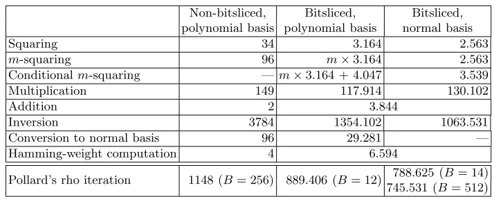
Non-bitsliced, Bitsliced, Bitsliced, polynomial basis polynomial basis normal basis
Squaring 34 3.164 2.563
m-squaring 96 m×3.164 2.563
Conditionalm-squaring —m×3.164 + 4.047 3.539
Multiplication 149 117.914 130.102
Addition 2 3.844
Inversion 3784 1354.102 1063.531
Conversion to normal basis 96 29.281 —
Hamming-weight computation 4 6.594
Pollard’s rho iteration 1148 (B= 256) 889.406 (B= 12) 788.625 (B= 14) 745.531 (B= 512)
Table 1.Cycle counts per input for all operations on one SPE of a 3192 MHz Cell Broadband Engine, rev. 5.1. For the bitsliced implementations, cycle counts for 128 inputs are divided by 128. The valueB in the last row denotes the batch size for Montgomery inversions.
Using the bitsliced normal-basis implementation—which uses DMA transfers to main memory to support a batch size of 512 for Montgomery inversions—on all 6 SPUs of a Sony Playstation 3 in parallel, we can compute 25.57 million iterations per second. The expected total number of iterations required to solve the ECDLP given in the ECC2K-130 challenge is 260.9 (see [2]). Using the software described in this paper, this number of iterations can be
computed in 2654 Playstation 3 years.
References
1. Daniel V. Bailey, Brian Baldwin, Lejla Batina, Daniel J. Bernstein, Peter Birkner, Joppe W. Bos, Gauthier van Damme, Giacomo de Meulenaer, Junfeng Fan, Tim G¨uneysu, Frank Gurkaynak, Thorsten Kleinjung, Tanja Lange, Nele Mentens, Christof Paar, Francesco Regazzoni, Peter Schwabe, and Leif Uhsadel. The certicom challenges ecc2-x. Presented at SHARCS 2009, 2009. http://eprint/XXX.
2. Daniel V. Bailey, Lejla Batina, Daniel J. Bernstein, Peter Birkner, Joppe W. Bos, Hsieh-Chung Chen, Chen-Mou Cheng, Gauthier Van Damme, Giacomo de Meulenaer, Luis Julian Dominguez Perez, Junfeng Fan, Tim G¨uneysu, Frank G¨urkaynak, Thorsten Kleinjung, Tanja Lange, Nele Mentens, Ruben Nieder-hagen, Christof Paar, Francesco Regazzoni, Peter Schwabe, Leif Uhsadel, Anthony Van Herrewege, and Bo-Yin Yang. Breaking ECC2K-130, 2009. http://eprint.iacr.org/2009/541.
3. Daniel J. Bernstein. Batch binary Edwards. InAdvances in Cryptology – CRYPTO 2009, volume 5677 of LNCS, pages 317–336, 2009.
4. Daniel J. Bernstein. Minimum number of bit operations for multiplication, May 2009. http://binary. cr.yp.to/m.html (accessed 2009-12-07).
5. Daniel J. Bernstein. Optimizing linear maps modulo 2. Workshop Record of SPEED-CC: Software Performance Enhancement for Encryption and Decryption and Cryptographic Compilers, 2009. http: //cr.yp.to/papers.html#linearmod2.
6. Daniel J. Bernstein and Tanja Lange. Explicit-formulas database. http://www.hyperelliptic.org/EFD/ (accessed 2010-01-05).
7. Eli Biham. A Fast New DES Implementation in Software. In FSE 1997, volume 1267 of LNCS, pages 260–272, 1997.
8. Joppe W. Bos, Marcelo E. Kaihara, Thorsten Kleinjung, Arjen K. Lenstra, and Peter L. Montgomery. On the security of 1024-bit RSA and 160-bit elliptic curve cryptography: version 2.1. Cryptology ePrint Archive, Report 2009/389, 2009. http://eprint.iacr.org/2009/389.
9. Joppe W. Bos, Marcelo E. Kaihara, and Peter L. Montgomery. Pollard rho on the PlayStation 3. In Workshop record of SHARCS’09, pages 35–50, 2009. http://www.hyperelliptic.org/tanja/SHARCS/ record2.pdf.
11. Robert P. Gallant, Robert J. Lambert, and Scott A. Vanstone. Improving the parallelized Pollard lambda search on anomalous binary curves. Mathematics of Computation, 69(232):1699–1705, 2000.
12. Darrel Hankerson, Alfred Menezes, and Scott A. Vanstone.Guide to Elliptic Curve Cryptography. Springer, New York, 2004.
13. Bernard Harris. Probability distributions related to random mappings. The Annals of Mathematical Statistics, 31:1045–1062, 1960.
14. H. Peter Hofstee. Power efficient processor architecture and the Cell processor. In HPCA 2005, pages 258–262. IEEE Computer Society, 2005.
15. IBM. IBM SDK for multicore acceleration (version 3.1). http://www.ibm.com/developerworks/power/ cell/downloads.html?S_TACT=105AGX16&S_CMP=LP.
16. IBM DeveloperWorks. Cell Broadband Engine programming handbook (version 1.11), May 2008. https: //www-01.ibm.com/chips/techlib/techlib.nsf/techdocs/1741C509C5F64B3300257460006FD68D. 17. Anatolii Karatsuba and Yuri Ofman. Multiplication of many-digital numbers by automatic computers.
Number 145 in Proceedings of the USSR Academy of Science, pages 293–294, 1962.
18. Peter L. Montgomery. Speeding the Pollard and elliptic curve methods of factorization. Mathematics of Computation, 48:243–264, 1987.
19. John M. Pollard. Monte Carlo methods for index computation (modp). Mathematics of Computation, 32:918–924, 1978.
20. Josef Stein. Computational problems associated with Racah algebra. Journal of Computational Physics, 1(3):397–405, 1967.
21. Joachim von zur Gathen, Amin Shokrollahi, and Jamshid Shokrollahi. Efficient multiplication using type 2 optimal normal bases. InArithmetic of Finite Fields – WAIFI 2007, volume 4547 ofLNCS, pages 55–68, 2007.