Common Randomness and Secret Key Capacities of
Two-way Channels
Hadi Ahmadi, Reihaneh Safavi-Naini
Department of Computer Science, University of Calgary, Canada {hahmadi, rei}@ucalgary.ca
Abstract. Common Randomness Generation (CRG) and Secret Key Establishment (SKE) are funda-mental primitives that are used in information-theoretic coding and cryptography. We study these two problems over the two-way channel model of communication, introduced by Shannon. In this model, the common randomness (CK) capacity is defined as the maximum number of random bits per channel use that the two parties can generate. The secret key (SK) capacity is defined similarly when the random bits are also required to be secure against a passive adversary. We provide lower bounds on the two capacities. These lower bounds are tighter than those one might derive based on the previously known results. We prove our lower bounds by proposing a two-round, two-level coding construction over the two-way channel. We show that the lower bound on the common randomness capacity can also be achieved using a simple interactive channel coding (ICC) method. We furthermore provide upper bounds on these capacities and show that the lower and the upper bounds coincide when the two-way channel consists of two independent (physically degraded) one-way channels. We apply the results to the case where the channels are binary symmetric.
Keywords:Two-way channel, wiretap channel, common randomness capacity, secret key capacity.
1
Introduction
Thetwo-way discrete memoryless channel(TWDMC) setup was initially proposed as a communication model by Shannon [25], where he studied the problem ofreliable message transmission (RMT) between two parties, here referred to as Alice and Bob. Shannon’s work brought about the foundation of multi-user information theory and attracted much attention in theory and practice. The TWDMC setup is a general two-party communication model where in each communication round both parties, simultaneously, provide inputs to the channel, and receive their corresponding outputs as (possibly probabilistic) functions of the two inputs. In each channel use, a TWDMC receives the inputs XA and XB from Alice and Bob and returns to them the outputs YA and YB, respectively. The channel is specified by the conditional distribution PYA,YB|XA,XB. In Reliable Message Transmission (RMT) using a TWDMC, Alice and Bob want to reliably send messages to each other. The reliable message (RM) rateRABfrom Alice to Bob isachievable if Alice can sendnRAB bits of message reliably
to Bob in nchannel uses; in analogy, an achievable RM rateRBA from Bob to Alice is defined. Accordingly, a
pair (RAB, RBA) is achievable if the two rates can be achieved using the TWDMC at the same time. The RM
capacity region is the set of all achievable pairs. An extension of RMT in the above setup when the two-way channel leaks information to a passive adversary, Eve, is calledsecure message transmission (SMT) over a two-way discrete memoryless wiretap channel (TWDMWC) [29]. Thesecure message (SM) capacity region for this problem is defined analogously to that of RMT, except that the messages are required to be both reliable and secure.
shared random variable. The common randomness (CR) rateRcris called achievable if the parties can generate nRcr shared random bits innchannel uses, and theCR capacity is the highest achievable CR rate.
The second problem issecret key establishment (SKE) over a TWDMWC, where Alice and Bob aim at calcu-lating a shared random variable that is unknown to the adversary, Eve. This problem can be seen as an extension of CRG when the two-way channel leaks information to Eve and the parties want their shared randomness to be secure from her. Accordingly, theSecret Key (SK) capacity is defined similarly to the CR capacity with the extra requirement that the randomness must satisfy reliability and security, both. This immediately induces the following question.
Question 1.What is the CR/SK capacity of an arbitrarily given two-way channel?
We remark that the two problems of RMT and CRG over TWDMCs are different in general: An RMT protocol is used to deliver given messages reliably to their destinations, while a CRG protocol produces shared randomness. However, these problems are related. In particular, when the parties have free access to independent sources of randomness (which is also assumed in this paper), any RMT protocol can be used to obtain a CRG protocol by Alice and Bob generating their random variables and sending them to each other reliably using RMT. A similar argument holds to relate SMT and SKE. As a consequence, an achievable pair (RAB, RBA) for
RMT (resp. SMT) results in an achievable rate RAB+RBA for CRG (resp. SKE). This leads to the following
natural question.
Question 2.Can the CR/SK capacity be obtained from the RM/SM capacity region by maximizingRAB+RBA
over all choices of (RAB, RBA)?
Certainly, this maximization suggests a lower bound on the CR/SK capacity; nevertheless, thistrivial lower bound may not be tight since the shared randomness could also be generated as a result of interaction between the two parties.
1.1 Our work
We give general descriptions of multi-round CRG and SKE protocols in the above setups and formally define the CR and the SK capacities. We first use the previous results on RMT and SMT, esp., those in [25, 29], to derive “trivial lower bounds” on the CR and the SK capacities. Next, we prove that the trivial bounds cannot be tight by giving a simple two-way channel example, where one bit of common randomness (or secret key) per channel use is achievable while the trivial bound is zero. We finally show that the lower bounds can be improved using interaction over the channel. The improved lower bounds on the CR and the SK capacities are achieved by a two-round construction that uses a two-level coding method, i.e., applying two sequential encoding functions to a message. However, we prove that the lower bound on the CR capacity can also be achieved using a two-round, but one-level,interactive channel coding (ICC) method, introduced in [6]. In both constructions, the first round involves sending independent and identically distributed (i.i.d.) random variables and the second round is used to send encoding information.
1.2 Related work
We first provide a selected summary of the literature on reliable/secure message transmission as related problems, and then discuss the work in the area of CRG and SKE. The systematic study of reliable message transmission over noisy channels is due to Shannon [24]. The problem has since been extended to many other communication setups, e.g., [1,8,25,30]. Shannon [25] introduced the two-way channel setup as an interesting scenario to model a two-party communication environment, and proved inner and outer bounds on the RM capacity region. In general, an inner bound contains a subset (not necessarily all) of the achievable pairs of RM rates (RAB, RBA),
whereas an outer bound is a superset of the set of all these pairs. The inner bound in [25] was shown not to be tight in [13] and was improved later in [15]. The outer bound was also improved in [33]; yet, due to the gap between the two bounds, finding the capacity region in this setup remains an open problem.
Transmission of secure messages over noisy channels was first considered by Wyner [31] and later discussed in several other setups, e.g., [10, 20, 27]. Secure message transmission over special cases of two-way wiretap channels was first investigated by Tekin and Yener [28, 29], where inner bounds on the SM capacity region were derived. The bounds were improved, more recently, in [14, 16, 21] using feedback and key exchange mechanisms as techniques to increase achievable rates.
The problem of two-party common randomness generation (CRG) has been previously studied in other setups, e.g., CRG over noiseless channels using correlated randomness [3, 12] or CRG over noisy channels [26], where the authors derived expressions for the CR capacity. Determining the CR capacity is important due to the role of common randomness in building two-party randomized protocols that, compared to deterministic protocols, have higher computation and communication efficiencies. Examples of such applications appear in random coding over arbitrarily varying channels (AVC) [11], identification over noisy channels [4], and oblivious transfer and bit commitment schemes [23, 32].
The CRG problem when the communication is over a hostile environment turns into the fundamental problem of secret key establishment (SKE) in cryptography: Alice and Bob want to share a common key about which an adversary Eve should be uncertain. The problem has been studied in numerous setups including noise-free public channels and noisy broadcast channels. The results on “secure transmission” over one-way wiretap channels [10, 31] imply the possibility of secure key establishment as long as the wiretap channel is not in Eve’s favor, e.g., adversary’s channel is noisier than the main channel. Maurer [18], concurrently with Ahlswede and Csisz´ar [2], showed that by assuming an additional noiseless public discussion channel, available to the parties in both ways, SKE may be possible even when the wiretap channel is in Eve’s favor. Noiseless channels in practice are realized from physical noisy channels using error correcting codes. Noting that this approach does not always lead to the highest achievable secret key rates, recent work studied SKE in setups that replace the above public discussion channel with other resources, e.g., a wiretap noisy channel in the opposite direction [5] or correlated sources of randomness [17, 22].
1.3 Discussion
In this paper, we prove lower and upper bounds on the CR and the SK capacities. The lower bound proofs use random coding arguments to show the existence of CRG and SKE constructions that achieve the bounds. One can, however, design practical constructions by using concrete primitives in the CRG/SKE protocols that are proposed in this paper. An example of such approaches to construct concrete protocols is the work in [7] that proposes a practical wireless key establishment scheme based on the theoretical results of [18, 31].
1.4 Notation
We use calligraphic letters (X), uppercase letters (X), and lowercase letters (x) to denote finite alphabets, random variables (RVs), and their realizations over sets, respectively. The size of X is denoted by|X |. Xn is
the set of all sequences of lengthn(so calledn-sequences) with elements fromX.Xn= (X
1, X2, . . . , Xn)∈ Xn
denotes a randomn-sequence inXn, andXj
i = (Xi, Xi+1, . . . , Xj) is a subsequence. To save space, we may use
boldXandxto denote a random sequence and its realization. For the RVsX,Y, andZ, we useX↔Y ↔Z
to denote a Markov chain between them. ‘||’ denotes concatenation of sequences. For a value x, we use [x]+ to
show max{0, x} and, for 0≤p≤1,h(p) =−plogp−(1−p) log(1−p) denotes the binary entropy function. Hereafter, we use the terms CRG and SKE specifically for the two-way (wiretap) channel setup.
1.5 Paper organization
Section 2 describes the two-way channel model, related problems, and current results. Section 3 summarizes our main results in the paper, including lower and upper bounds and their coincidence. In Section 4, we briefly present our CRG and SKE constructions that achieve the lower bounds on the CR and the SK capacities. Section 5 applies the lower bound results to the case of two-way binary channels. We conclude the paper in Section 6.
2
Model and Definitions
2.1 CRG in the TWDMC setup
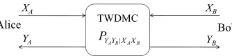
Alice and Bob are connected by a Two-Way Discrete Memoryless Channel (TWDMC) that is denoted by (XA, XB)→(YA, YB) and specified by the conditional probability distributionPYA,YB|XA,XB over the finite sets XA,XB,YA,YB. The channel is indicated in Fig. 1. We furthermore assume that each party has free access to
an independent source of randomness.
XA
Bob Alice
XB
TWDMC
YA PYAYB|XAXB YB
Fig. 1.The Two-Way Discrete Memoryless Channel (TWDMC) setup.
Alice and Bob follow a Common Randomness Generation (CRG) protocol over the TWDMC to generate a shared random variable. In general, the protocol consists of a certain number of communication rounds, denoted byt. In each round, 1≤r≤t, Alice and Bob send sequences of random variables (RVs)X:r
lengthnr, and receive thenr-sequencesYA:randYB:r, respectively. The sequenceX:Ar(resp.X:Br) is determined as
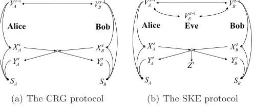
a function of some independent randomness and the previously communicated (sent and received) sequences by Alice (resp. Bob). At the end of roundr, the view of each party from the protocol is the set of their communicated sequences. Letting V:r
A andVB:r be respectively the views of Alice and Bob at the end of roundr, we have V:r
A =||ri=1 X:Ai||Y
:i A
, V:r
B =||ri=1 X:Bi||Y
:i B
. (1)
Finally,V iewA =VA:t and V iewB =VB:t are the views at the end of the last communication round. Alice
usesV iewAto calculateSA∈ S and Bob usesV iewB to calculateSB∈ S. The total number of channel uses is
calculated as
n=
t
X
r=1
nr. (2)
Fig. 2(a) indicates the relationship between the final randomness and the views of the parties in rounds t
andt−1 of a CRG protocol. For instance, Alice calculatesX:t
A based on her viewV
:t−1
A asXA:t=f(Rt, VA:t−1),
wheref is a deterministic function andRtis her local randomness that is used in roundtand is independent of
the views in round t−1. This means that, givenVA:t−1,X:t
A is independent ofV
:t−1
B which implies the Markov
chainV:t−1
B ↔V
:t−1
A ↔XA:t. In a similar way, one can derive Markov chains between other sets of variables in
a general CRG protocol. These Markov chains are later used in proving of an upper bound on the capacity.
Bob 1
:t A
V :t1
B V Alice Bob t B X: t A X: Alice S S t B Y: t A Y: A
S SB
(a) The CRG protocol
Bob 1
:t A
V :t1
B V 1 :t E V
Alice Eve Bob
t B X: t A X: Alice Eve S S t B Y: t A Y: t Z: A
S SB
(b) The SKE protocol
Fig. 2.The relationship between variables in the CRG/SKE protocol
Definition 1. For Rcr ≥0 and 0 ≤δ ≤1, the CRG protocol Π in the TWDMC setup is (Rcr, δ)-reliable if
there exists a random variable S∈ S such that
H(S)
n > Rcr−δ, (3)
Pr(SA=SB =S)>1−δ. (4)
Definition 2. The common randomness (CR) rate Rcr ≥ 0 in the TWDMC setup is achievable if for an
arbitrarily small δ >0, there exists an (Rcr, δ)-reliable CRG protocol. The CR capacityin this setup is denoted
by CT W DM C
cr and is defined as the highest achievable CR rate.
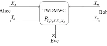
2.2 SKE in the TWDMWC setup
TWDMWC
XA
Bob Alice
XB
YA YB
B A B AYZX X
Y
P |
Z
Eve
Fig. 3.The Two-Way Discrete Memoryless Wiretap Channel (TWDMWC) setup.
Bob, and the adversary, Eve, respectively. The channel is specified by the conditional distributionPYA,YB,Z|XA,XB over the finite setsXA,XB,YA,YB,Z. Again, the parties have free access to independent sources.
A general t-round SKE protocol in this setup is described analogously to a general CRG protocol except that, in each roundr, Eve receives annr-sequenceZ:rand her view at the end of this round is written as
VE:r=||ri=1Z:i. (5)
Eve’s view at the end of the protocol isV iewE=VE:t. Fig. 2(b) shows how the parties’ views in roundt−1 and t are related to the keys, calculated by Alice and Bob.
Definition 3. For Rsk ≥0 and 0 ≤δ ≤1, the SKE protocol Π in the TWDMWC setup is (Rsk, δ)-secure if
there exists a random variable S∈ S such that
H(S)
n > Rsk−δ, (6)
Pr(SA=SB=S)>1−δ, (7)
H(S|V iewE)
H(S) >1−δ. (8)
Definition 4. The secret key (SK) rate Rsk ≥0 in the TWDMWC setup is achievable if for an arbitrarily
small δ >0, there exists an (Rsk, δ)-secure SKE protocol. The secret key capacity in this setup is denoted by CT W DM W C
sk and is defined as the highest achievable SK rate.
Remark 1. The above definition of SK capacity follows those in [2, 10, 17, 18, 22, 31]. This definition is referred to asthe weak SK capacity as it requires Eve’s uncertainty rate about the secret key to be negligible (as in (8)), whereas the “strong” SK capacity [19] requires Eve’s total uncertainty to be negligible, i.e., requiring
H(S|V iewE)> H(S)−δ. (9)
It is shown [19] that, for the setups in [10, 18, 31], the weak definition can be replaced by the strong definition without sacrificing the SK capacity. This result can also be extended to the TWDMBC setup by modifying the proof in [19]. This is left as future work.
2.3 Known results on two-way channels
Shannon’s work [25] on reliable message transmission (RMT) over TWDMCs proved the following inner bound,
GI, and outer bound, GO, on the RM capacity region of the channel (XA, XB) → (YA, YB). Letting P = PXA,XB,YA,YB,
R(P) ={(RAB, RBA) :RAB ≤I(XA;YB|XB), RBA≤I(XB;YA|XA)},
GI =SPXA,XB=PXA.PXBR(P), (10)
where, by ∪, we mean the convex closure of the union of R(P)’s. The bound on RAB (if maximized w.r.t. PXA,XB) somehow reflects the capacity of the one-way channelXA→YBfrom Alice to Bob whenXB is known to Bob; similarly, one can interpret the bound on RBA. The two inner and outer bounds in (10) and (11) have
been later discussed and slightly improved (see, e.g., [13, 15, 33]).
Tekin and Yener [28, 29] considered secure message transmission (SMT) over Gaussian and binary two-way wiretap channels. The authors proved the following set of achievable pairs as an inner bound on the SM capacity region. Letting P =PXA,XB,YA,YB,Z,
Rs(P) ={ (Rs,AB, Rs,BA) :Rs,AB ≤[I(XA;YB|XB)−I(XA;Z)]+, Rs,BA≤[I(XB;YA|XA)−I(XB;Z)]+,
Rs,AB+Rs,BA≤[I(XA;YB|XB) +I(XB;YA|XA)−I(XA, XB;Z)]+ },
Gs,I=SP
XA,XB=PXA.PXBRs(P). (12) The bound on Rs,AB (if maximized w.r.t. PXA,XB) shows the SM capacity of the channel XA → (YA, Z) when XB is known to Bob; similar is the bound on RBA. It is noteworthy that the inner bound (12) has
been improved in [14, 16, 21] using techniques such as feedback and key exchange mechanisms in addition to cooperative jamming.
2.4 Two-way channels with independent components
A special class of TWDMCs includes those which consist of two independent DMCs in the two directions, i.e.,
PYA,YB|XA,XB =PYB|XA.PYA|XB.
We refer to this class as2DMC. The CRG problem in this setup when Alice and Bob have “limited” access to independent sources of randomness has been considered in [26], where a single letter formula for the capacity was determined.
Likewise, 2DMWCs refer to a class of TWDMWCs that consist of two independent DMWCs in opposite directions. More precisely, a TWDMWC (XA, XB)→(YA, YB, Z) is a 2DMWC when
Z= (Z1, Z2), and
PYA,YB,Z|XA,XB =PYB,Z1|XA.PYA,Z2|XB.
The SKE problem in this setup has been recently studied in [5], where lower and upper bounds on the SK capacity were provided and were shown to coincide when each DMWC is physically degraded. Informally, in a physically degraded DMWC, one of the receivers always receives a noisy version (though a noisy channel) of what the other receiver receives. This can be modeled using a Markov chain. e.g., the Markov chainX↔Y ↔Z
indicates a degraded channel where Y is a noisy version of the input X and Z (as a noisy version of Y) is a noisier version of X. This Markov chain impliesI(X;Z|Y) = 0.
Definition 5. The DMWCX→(Y, Z)is called obversely degradedif X↔Y ↔Z forms a Markov chain. It is called reversely degradedif X ↔Z ↔Y forms a Markov chain. The DMWC is called physically degraded if we can write X= [XO, XR],Y = [YO, YR], andZ= [ZO, ZR], where
ZO↔YO↔XO↔XR↔ZR↔YR
holds.
3
Statement of the Main Results
3.1 Trivial lower bounds and a TWDMC example
From (10) and (12), we can derive trivial lower bounds on the CR and the SK capacities, respectively. Again, note that if (RAB, RBA) is an achievable RM/SM rate, thenRAB+RBA is an achievable CR/SK rate. As a
consequence, the two following expressions respectively give trivial lower bounds on the CR capacity,CT W DM C
cr ,
and the SK capacity,CT W DM W C
sk .
CcrT W DM C ≥ max
PXA,XB=PXA.PXB[I(XA;YB|XB) +I(XB;YA|XA)], (13)
CskT W DM W C ≥ max
PXA,XB=PXA.PXB[[I(XA;YB|XB)−I(XA;Z)]++ [I(XB;YA|XA)−I(XB;Z)]+]. (14)
One may ask whether the above trivial lower bounds cannot be improved or, more generally, whether the RM/SM capacity region specifies a tight lower bound on the CR/SK capacity, by maximizingRAB+RBAover
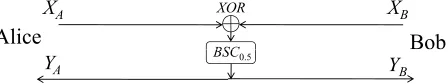
all choices of achievable pairs. We give a negative answer to this question using the following simple example. Consider the TWDMC shown in Fig. 4 which is a modified version of Shannon’s modulo-two additive two-way channel example [25, Fig. 4], where there exists a binary symmetric channel (BSC) with bit error probability
1
2, right after the XOR operand. In this example, the channel outputs are independent of the inputs; hence,
little chance of reliable message transmission. This implies that no pair of rates except (RAB= 0, RBA= 0) is
achievable; in this case, the inner bound (10) is tight and represents the capacity region.
BSC
XA
!"
#$%&'
XB
XOR
BSC()*
YA YB
Fig. 4.A TWDMC example.
Using (13), which is obtained from (10), we derive a “zero” lower bound on the CR capacity. However, this lower bound is not tight since Alice and Bob can share one random bit (YA = YB) each time they use the
channel. The key observation is that the common randomness is a function of channel noise and the parties’ inputs, and it does not need to be selected a priori by the parties. Since RMT and CRG in TWDMC are viewed respectively as special cases of SMT and SKE in TWDMWC, the above example also lets us conclude that the SM capacity region of a TWDMWC does not necessarily give a tight lower bound on the SK capacity in general.
3.2 Common randomness capacity
We provide lower and upper bounds on the CR capacity in the TWDMC setup, present give our informal inter-pretation of the expressions. Let the RVsXA, YA, XB, andYBcorrespond to the channel probability distribution PYA,YB|XA,XB. LetUA andUB be random variables from arbitrary setsUA andUB such that
UA↔(XA, YA)↔(XB, YB)↔UB
Theorem 1. The CR capacity in the TWDMC setup is lower bounded as
CT W DM C
cr ≥maxn1,n2,PUA,XAPUB ,XB[n1[I(UA;XB,YB)+I(UB;XA,YA|UnA)]+n2[I(XA;YB,XB)+I(XB;YA,XA)]
1+n2 , (15)
s.t. PXA,XB=PXA.PXB, (16)
n1I(UA;XA, YA|XB, YB)< n2I(XA;XB, YB), (17)
n1I(UB;XB, YB|XA, YA)< n2I(XB;XA, YA)]. (18)
Proof. See Appendix A.
Remark 2. Since XA and XB are independent, the second term can also be written as n2[I(XB;YA|XA) + I(XA;YB|XB)]; hence, whenn1= 0 the argument equals that of (13). This shows that the new lower bound is
greater than or equal to the trivial lower bound in (13).
Remark 3. The above lower bound is achieved using a two-round coding construction (as in Appendix A). The terms in (15) can be interpreted as follows. The first term n1[I(UA;XB, YB) +I(UB;XA, YA|UA)] shows
the amount of raw (uncoded) correlated information that is provided in the first communication round with
n1 channel uses. This information is obtained based on the inputs and the outputs of the channel. The second
termn2[I(XB;YA, XA)+I(XA;YB, XB)] indicates the amount of correlated information, provided in the second
communication round, following the coding construction. This information equals the sum of the RM rates of the channel in both directions (i.e., the bounds on RAB andRBAin (10)). The conditions (17) and (18) mean
that the amount of confusion (uncertainty) about the transmitted information in the first round can not be more than the capability of the channel for reliable transmission in the second round.
The next theorem determines an upper bound on the CR capacity in the TWDMC setup, i.e., the highest CR rate that all CRG protocols can achieve.
Theorem 2. The CR capacity in the TWDMC setup is upper bounded as
CcrT W DM C ≤ max
PXA,XB[I(XB;YA|XA) +I(XA;YB|XB) +I(YA;YB|XA, XB)]. (19)
Proof. See Appendix B.
Remark 4. The first two terms of (19) are the same as those of (11) for the RM capacity region. The third term, however, is due to the exclusive property of CRG that the common randomness may be obtained from the correlated information between the outputs. This again articulates the essential difference between the two problems in the TWDMC setup.
Definition 6. A (bipartite) systematic channel code, with encoding alphabets (T,U) and decoding alphabets (V,W), is a pair of encoding/decoding functions(Enc/Dec), where
– Enc : Tn1 × Un2,i → Vn1 × Wn2 deterministically maps (tn1||un2,i) (as the information sequence) to a sequence (tn1||un2), such that (un2 = un2,i||un2,p) and n
2 = n2,i+n2,p; we call un2,p the parity check
sequence.
– Dec:Vn1× Wn2→ Tn1× Un2,i assigns a guess sequence(ˆtn1||ˆun2,i)to each input(vn1||wn2).
The ICC method has been proposed in [6] and was shown to be useful in achieving the lower bound on the SK capacity of a 2DMWC under certain conditions [6].
Theorem 3. The lower bound (15) on the CR capacity can be achieved using the one-level interactive channel coding method.
Proof. See Section 4.2 and Appendix C.
In the following, we consider the 2DMC setup as described in Section 2.4, and show that the lower and the upper bounds on the CR capacity coincide for this class of TWDMCs. We note that the CR capacity (20) matches the result in [26], on CRG over 2DMCs, when there is no limit on the available independent randomness.
Proposition 1. When the TWDMC consists of two independent DMCs in the two directions (called a 2DMC), the two bounds coincide and the CR capacity equals
C2DM C
cr = max
PXA,PXB
{I(XA;YB) +I(XB;YA)}. (20)
Proof. See Appendix D.
Proposition 1 implies that, in the 2DMC setup, the RM capacity region, e.g., obtained from the results of [25] (see (10)), can be used to obtain the CR capacity (i.e., a tight lower bound), by solving the sum maximization problem.
3.3 Secret key capacity
We provide lower and upper bounds on the SK capacity in the TWDMWC setup. These bounds are gener-alizations of the bounds, given in Section 3.2, to the cases when the communication is eavesdropped by Eve. Let the RVsXA, YA, XB, YB, andZ correspond to the channel probability distributionPYA,YB,Z|XA,XB and let
UA, W1A, W2A, UB, W1B, andW2B be random variables from arbitrary setsUA,W1A,W2A,UB,W1B, andW2B,
respectively, such that the following Markov chains hold,
UA↔(XA, YA)↔(XB, YB)↔UB, (21)
W2A↔W1A↔XA↔(XB, YA, YB, Z), (22)
W2B ↔W1B↔XB ↔(XA, YA, YB, Z). (23)
Theorem 4. The SK capacity in the TWDMWC setup is lower bounded as
CskT W DM W C≥ max
n1,n2,PW2A ,W1A ,UA ,XAPW2B ,W1B ,UB ,XB [ 1
n1+n2
(n1[I(UA;XB, YB) +I(UB;XA, YA|UA)−I(UA, UB;Z)]
+n2[I(W1A;XB, YB|W2A) +I(W1B;XA, YA|W2B)−I(W1A, W1B;Z|W2A, W2B)]+), (24)
s.t. PXA,XB =PXA.PXB (25)
n1I(UA;XA, YA|XB, YB)< n2I(W1A;XB, YB), (26)
Proof. See Section 4.1 and Appendix A.
The terms in (24) can be interpreted in analogy to the argument following (15), adding that the shared information is required to remain secure from Eve and, hence, a privacy amplification is needed. Informally, the terms n1I(UA, UB;Z) and n2I(W1A, W1B;Z|W2A, W2B) show the amount of leakage of shared randomness in
the first and the second rounds, respectively.
The upper bound on the SK capacity is provided in the following. Let Q be a random variable from an arbitrary setQ such that
Q↔(XA, XB)↔(YA, YB, Z)
forms a Markov chain.
Theorem 5. The SK capacity in the TWDMWC setup,CT W DM W C
sk , is upper bounded by
max
PQ,XA,XB[I(XA;YB|XB, Z) +I(XB;YA|XA, Z) +I(YA;YB|XA, XB, Z) +I(XA;XB|Z, Q)−I(XA;XB|Q)]. (28)
Proof. See Appendix B.
The following proposition states that if the TWDMWC consists of two independent DMWCs with degraded channels (see Section 2.4), then the lower and the upper bounds coincide and the SK capacity is achieved by a one-round protocol. In [5], SKE over 2DMWCs has been considered in the half-duplex communication model where the two forward and backward channels could be used for different number of times. The following special case of TWDMWC, however, complies a full-duplex communication model where the channels are used together and the number of channel uses must be the same for the two channels. The results in [5] are consistent to those in Proposition 2, assuming the full-duplex communication model.
Proposition 2. When the 2DMWC consists of degraded DMWCs XA↔YB↔Z1 andXB↔YA↔Z2(as in
Definition 5), the lower bound coincides with the upper bound, and the SK capacity equals
C2DM W C
sk = max
PXA,PXB
{I(XA;YB|Z1) +I(XB;YA|Z2)}. (29)
Furthermore, the SK capacity is achieved by a one-round protocol. Proof. See Appendix D.
4
CRG/SKE Protocol Outline
The complete structure of the protocols are described in the lower bound proofs in the appendix. In this section, we present a brief explanation to give the intuition behind these constructions.
4.1 The two-round CRG/SKE protocol (Theorems 1 and 4)
For simplicity, we give an outline of the SKE protocol in the following special case: W1A =XA,W1B =XB, W2A =W2B = 0, and the two conditions in (26) and (27) hold with almost equality. Letn1,n2, PUA,XA, and
PUB,XB be those that maximize the right side of (24), which is written as
Rsk= n 1
1+n2(n1[I(UA;XB, YB) +I(UB;XA, YA|UA)−I(UA, UB;Z)]
+n2[I(XA;XB, YB) +I(XB;XA, YA)−I(XA, XB;Z)]+). (30)
Define
ηa,f ≈n1I(UA;XA, YA), ηa,t≈n2I(XA;XB, YB) (31)
ηb,f ≈n1I(UB;XB, YB), ηb,t≈n2I(XB;XA, YA), (32)
– Let Un1
A,ǫ (resp. U n1
B,ǫ) be obtained by randomly and independently choosing 2ηa,f (resp. 2ηb,f) typical
se-quences fromUn1
A (resp.U n1
B ).
– Let {Un1
A,ǫ,i}2
ηa,t
i=1 be a partition ofUA,ǫn1 into 2ηa,t equal-sized parts. Define the functiontA : UA,ǫn1 → TA =
{1,2, . . . ,2ηa,t} such that, for any input in Un1
A,ǫ,i, it outputs i. Similarly define the partition {U n1
i,B,ǫ}2
ηb,t
i=1
and the functiontB.
– Let{Ks}2
κ
s=1be a partition ofUA,ǫn1 × U n1
B,ǫinto equal-sized parts of size 2γ. Define the key derivation function φ:Un1
A,ǫ× U n1
B,ǫ→ {1,2, . . . ,2κ}such that, for any input inKs, it outputss.
The protocol proceeds in two rounds. In round 1, Alice and Bob send i.i.d.n1-sequencesX:1AandX:1Baccording
toPXA andPXB, and receive then1-sequencesY
:1
A andY:1B, respectively, while Eve receivesZ:1. Alice searches
inUn1
A,ǫto find a sequenceU n1
A that is jointly typical to (X
:1
A,YA:1) w.r.t.P(XA,YA),UA. Similarly, Bob searches for a sequenceUn1
B that is jointly typical to (X:1B,YB:1) w.r.t.P(XB,YB),UB. Now, (U
n1
A , U n1
B ) represents the common
randomness that needs to be made reliable in the second round.
In round 2, Alice computes TA = tA(UAn1), which can help Bob decode his (X
:1
B,YB:1) to UAn1. Bob also
computesTB=tB(UBn1). Alice and Bob encodeTAandTB ton2-sequencesX:2A=Enc(TA) andX:2B=Enc(TB)
and send them over the channel. The parties and Eve receiveY:2
A,Y:2B, andZ:2, respectively. Alice first decodes
(X:2
A,Y:2A) to ˆTB ≈TB, and uses this for decoding (X:1A,Y:1A) to ˆU n1
B ≈U
n1
B . The decoding function relies on the
jointly-typical decoding technique for long sequences (see, e.g., [9, Chapter 8]). Similarly Bob finds ˆTA≈TAand
then ˆUn1
A ≈U
n1
A . Now, the parties have a reliable common randomness, but it is not perfectly secure against
Eve. To derive a secret key, the parties compute φ(Un1
A , U n1
B ). The rest of the proof is to show that there exist
encoding/decoding functions and a key derivation function for the above construction with parameters (31)-(33), such that the protocol achieves the lower bound (24) and satisfies reliability and secrecy requirements (7) and (8) for an arbitrarily smallδ >0.
4.2 The CRG construction using the ICC method (Theorem 3)
Again for simplicity, let the two conditions in (17) and (18) hold with almost equality. Also letn1,n2,PXA, and
PXB be those that maximize the right side of (15). The protocol has two rounds. The first round is the same as that in Section 4.1, and so the common randomness is defined to be (Un1
A , U n1
B ). However, the second round
differs as follows.
Alice and Bob use their systematic coding functions to encode (Un1
A ,X:2A) = Enc(U n1
A ) and (U n1
B ,X:2B) = Enc(Un1
B ), respectively. Next, they send the parity-check sequencesX:2AandX:2B, and receiveY:2AandYB:2. Using
the bipartite jointly typical decoding method (see Appendix C), Alice decodes (X:1
A,Y:1A,X:2A,Y:2A) to ˆU n1
B ≈U
n1
B ,
and Bob decodes (X:1
B,YB:1,X:2B,Y:2B) to ˆU n1
A ≈U
n1
A . Overall, the common randomness isS = (U n1
A , U n1
B ): Alice
obtains SA= (UAn1,UˆBn1), and Bob obtainsSB= ( ˆUAn1, UBn1). Appendix C shows that the rate achieved by this
construction matches the lower bound in (15) and the protocol satisfies the reliability requirement (4) for an arbitrarily smallδ >0.
5
Achievable Rates over Two-Way Binary Wiretap Channels
Consider the Two-Way Binary Wiretap Channel (TWBWC) setup as in Fig. 5, where the inputs and the outputs are binary variables. In this model, the two input bits XA and XB to the channel are XORed (added modulo
the input bits as
YA=XA+XB+NrA, (34)
YB=XA+XB+NrB, (35)
Z=XA+XB+NE, (36)
where + indicates modulo-two addition.
XA
Bob Alice
XB
Bob
YA YB
N NE N
Z
Eve
NrA NE NrB
Fig. 5.Two-way binary wiretap channel.
In this section, we study the behavior of the lower bounds, proved in Section 3, for the case of binary channels and compare them to the trivial lower bounds that are obtained based on the previous work on message transmission. Since the CRG problem can be viewed as a spacial case of SKE, where Eve receives no information about the transmitted sequences (i.e., when pe = 0.5), we only focus on the SKE problem.
Throughout, for two real values 0≤x, y ≤1, we use x ⋆ yto denote the error probability in the cascade of two BSCs with error probabilitiesxandy, i.e.,
x ⋆ y=x+y−2xy.
The following lemma indicates the the cascade of any two BSCs is noisier, compared to each of them.
Lemma 1. For any real values 0≤x, y≤1, we have
|x ⋆ y−0.5| ≤min{|x−0.5|,|y−0.5|}, (37)
and
h(x ⋆ y)≥max{h(x), h(y)}. (38)
Proof. See Appendix E.
We use Theorem 4 to obtain a lower bound,LboundN, on the SK capacity in the above model.
Lemma 2. The SK capacity in the TWBWC setup is lower bounded as
CskT W BW C ≥LboundN
△
= max
0≤p1,p2≤1
[µL1+ (1−µ)[L2]+], (39)
where
L1= 1 +h(p1⋆ p2⋆ pra⋆ prb⋆ pe)−h(p1⋆ pra)−h(p2⋆ prb), (40)
L2= 1 +h(p1⋆ p2⋆ pe)−h(p1⋆ pra)−h(p2⋆ prb), (41)
µ= min{ 1−h(p1⋆ pra) 1−h(p1⋆ pra) +h(p2⋆ prb)
, 1−h(p2⋆ prb) 1−h(p2⋆ prb) +h(p1⋆ pra)
furthermore,
LboundN ≥ max
0≤p1,p2≤1
[L2]+. (43)
Proof. See Appendix F.
Remark 5. Lemma 2 provides a lower bound on the SK capacity that dominates the trivial lower bound, achieved from the previous work. This is shown in the sequel. Nevertheless, the lower bound (39) is not the highest rate one can obtain from the results of Theorem 4; in other words, one may use the result of Theorem 4 to derive a tighter lower bound in the TWBWC model. This is left as future work.
Secure message transmission in the above TWBWC model has been considered in [14, 28]. We choose to study the results in [14], which provide a strictly larger achievable rate region for secure message transmission. The achievable rate region in [14] is given as follows:
Gs,I= convex hull of {(Rs,AB, Rs,BA), s.t. ∃0≤p1, p2≤1 : Rs,AB ≤1−h(p2⋆ prb), Rs,BA≤1−h(p1⋆ pra),
Rs,AB+Rs,BA≤[1 +h(p1⋆ p2⋆ pe)−h(p1⋆ pra)−h(p2⋆ prb)]+}. (44) This implies the following lower bound on the SK capacity.
LboundT = max
(Rs,AB,Rs,BA)∈Gs,I
[Rs,AB+Rs,BA]
= max
0≤p1,p2≤1[1 +h(p1⋆ p2⋆ pe)−h(p1⋆ prb)−h(p2⋆ pra)]+ = max
0≤p1,p2≤1[L2]+, (45)
where the last equality follows from (41). Comparing (43) and (45) leads to the following corollary.
Corollary 1. The lower bound (39), proved in this paper, on the SK capacity in the TWBWC setup is always greater than or equal to the trivial lower bound (45), i.e.,
LboundN ≥LboundT. (46)
0 0.1 0.2 0.3 0.4 0.5
0 0.2 0.4 0.6 0.8 1 1.2 1.4 1.6 1.8 2
Receiving channel error probability, p r L o w er b o u n d v a lu es o n t h e S K c a p a ci ty Lbound N Lbound T
(a) 0≤pr≤0.5 andpe= 0.1
0 0.1 0.2 0.3 0.4 0.5
0 0.2 0.4 0.6 0.8 1 1.2 1.4 1.6 1.8 2
Eavesdropping channel error probability, pe
L o w er b o u n d v a lu es o n t h e S K c a p a ci ty Lbound N Lbound T
(b) 0≤pe≤0.5 andpr= 0.1
Fig. 6.Comparison of the lower bound values with respect to the error probabilities.
To better understand the gap between the trivial lower boundLboundT and the newly proved lower bound LboundN, we evaluate these two quantities with respect to different choices of channel error probabilities in Fig.
the receiving channel noise for Alice and Bob is the same, i.e.,pra=prb=pr. Fig. 6(a) compares the two lower bound values with respect topr whenpe= 0.1. Observe the non-zero gap between LboundN andLboundT for
receiving channel noise pr<0.15. This confirms that the lower bounds proved in this paper strictly dominate
those which can be obtained using the previous results on secure message transmission. Fig. 6(b) compares the bound values as functions ofpewhenpr= 0.1. It shows the gap between the two bounds expect for much small
or much large values of the eavesdropping channel error probability pe.
6
Conclusion
We considered the two-way channel setup and studied the problems of common randomness generation and secret key establishment for the first time in this setup. We discussed the relation between the above problems and reliable/secure message transmission over two-way channels, which are previously studied in the literature. We defined the common randomness and the secret key capacities and derived trivial lower bounds on these capacities based on the previously known results. Next, we showed that these trivial lower bounds can be improved by proposing two-round protocols that can achieve higher rates of common randomness/secret key. We applied the results to the case of two-way binary channels, where we showed the gap between the trivial lower bounds and those derived in this paper. We also proved upper bounds on the capacities and discussed the cases that the lower and the upper bounds coincide. It has not been shown whether any of the bounds are tight in general, or more specifically, whether one can improve the bounds by allowing more rounds of interaction. These open questions proffer directions to future work.
References
1. Ahlswede, R.: Multi-way communication channels. In: 2nd International Symposium Information Theory, pp. 103135 (1971)
2. Ahlswede, R., Csisz´ar, I.: Common randomness in information theory and cryptography. Part I: secret sharing. IEEE Transactions on Information Theory, vol. 39, pp. 1121-1132 (1993)
3. Ahlswede, R., Csisz´ar, I.: Common randomness in information theory and cryptography. Part II: CR capacity. IEEE Transactions on Information Theory, vol. 44, pp. 225-240 (1998)
4. Ahlswede, R., Dueck, G.: Identification via channels. IEEE Transactions on Information Theory, vol. 35, pp. 15-29 (1989)
5. Ahmadi, H., Safavi-Naini, R.: Secret key establishment over a pair of independent broadcast channels. In: International Symposium Information Theory and its Application, 2010. Full version on the arXiv preprint server, arXiv:1001.3908 6. Ahmadi, H., Safavi-Naini, R.: New results on key establishment over a pair of independent broadcast channels. In: International Symposium Information Theory and its Application, 2010. Full version on the arXiv preprint server, arXiv:1004.4334v1
7. Bloch, M., Barros, J., Rodrigues, M.R.D., McLaughlin, S.W.: Wireless Information Theoretic Security. IEEE Trans-actions on Information Theory, vol. 54, pp. 2515-2534 (2008)
8. Cover, T.M.: Broadcast channels. IEEE Transactions on Information Theory, vol. 18, pp. 2-14 (1972) 9. Cover, T.M., Thomas, J.A.:Elements of Information Theory. Wiley-IEEE, Edition 2 (2006)
10. Csisz´ar, I., K¨orner, J.: Broadcast channels with confidential messages. IEEE Transactions on Information Theory, vol. 24, pp. 339-348 (1978)
11. Csisz´ar, I., Narayan P.: The capacity of the arbitrarily varying channel revisited: positivity, constraints. IEEE Trans-actions on Information Theory, vol. 34, pp. 181-193 (1988)
13. Dueck, G.: The capacity region of the two-way channel can exceed the inner bound. Information and Control, vol. 40, pp. 258266 (1979)
14. El Gamal, A., Koyluoglu, O.O., Youssef, M., El Gamal, H.: The two way wiretap channel: theory and practice. Available on the arXiv preprint server, arXiv:1006.0778v1 (2010)
15. Han, T.S.: A general coding scheme for the two-way channel. IEEE Transactions on Information Theory, vol. 30, pp. 3544 (1984)
16. He, X., Yener, A.: The role of feedback in two-way secure communications. Available on the arXiv preprint server, arXiv:0911.4432v1 (2009)
17. Khisti, A., Diggavi, S., Wornell, G.: Secret key generation with correlated sources and noisy channels. In: IEEE International Symposium Information Theory (ISIT), pp. 1005-1009 (2008)
18. Maurer U.: Secret key agreement by public discussion from common information. IEEE Transactions on Information Theory, vol. 39, pp. 733-742 (1993)
19. Maurer, U., Wolf, S.: Information-theoretic key agreement: from weak to strong secrecy for free. In: Eurocrypt, LNCS 1807, pp. 351-351 (2000)
20. Oohama, Y.: Coding for relay channels with confidential messages. In: IEEE Information Theory Workshop, pp. 8789 (2001)
21. Pierrot, A.J., Bloch, M.R.: Strongly secure communications over the two-Way wiretap channel. Available on the arXiv preprint server, arXiv:1010.0177v1 (2010)
22. Prabhakaran, V., Eswaran, K., Ramchandran, K.: Secrecy via sources and channels - a secret key - secret message rate trade-off region. In: IEEE International Symposium Information Theory (ISIT), pp. 1010-1014 (2008)
23. Rivest, R.L.: Unconditionally secure commitment and oblivious transfer schemes using private channels and a trusted initializer, 1999. Available online at:http://theory.lcs.mit.edu/ rivest/Rivest-commitment.pdf.
24. Shannon, C.E.: A mathematical theory of communication. Bell System Technical Journal, vol. 27, pp. 379423 and 623656 (1948)
25. Shannon, C.E.: Two-way communication channels. In: 4th Berkeley Symposium on Mathematical Statistics and Probability, vol. 1, pp. 611644 (1961)
26. Venkatesan, S., Anantharam, V.: The common randomness capacity of a pair of independent discrete memoryless channels. IEEE Transactions on Information Theory, vol. 44, pp. 215224 (1998)
27. Tekin E., Yener, A.: The Gaussian multiple-access wire-tap channel with collective secrecy constraints. In: IEEE International Symposium Information Theory (ISIT), pp. 11641168 (2006)
28. Tekin E., Yener, A.: Achievable rates for two-way wire-tap channels. In: IEEE International Symposium on Infor-mation Theory (ISIT), pp. 941-945 (2007)
29. Tekin E., Yener, A.: The general Gaussian multiple access channel and two-way wire-tap channels: achievable rates and cooperative jamming. IEEE Transactions on Information Theory, vol. 54, pp. 2735-2751 (2008)
30. Van Der Meulen, E.C.: Three-terminal communication channels. In: Advances in Applied Probability, Vol. 3, pp. 120-154 (1971)
31. Wyner, A.D.: The wire-tap channel. Bell System Technical Journal, vol. 54, pp. 1355-1367 (1975)
32. Winter, A., Nascimento, A.C.A., Imai, H.: Commitment capacity of discrete memoryless channels. In: Cryptography and Coding, LNCS 2898, pp. 3551 (2003)
33. Zheng, Z., Berger, T., Schalkwijk, J.P.M.: New outer bounds to capacity region of two-way channels. IEEE Trans-action Information Theory, vol. 32, pp. 383-386 (1986)
A
Proving Theorems 1 and 4
We prove Theorem 4 and the proof of Theorem 1 follows as a special case where there is no adversary, i.e.,
Z = 0, and when we chooseW1A=XA, W1B=XB, andW2A=W2B= 0.
LetRsk be the expression to be maximized on the right side of (24), i.e., Rsk=n 1
1+n2(n1[I(UA;XB, YB) +I(UB;XA, YA|UA)−I(UA, UB;Z)]
Also let (26) and (27) be respectively rephrased as
n1[I(UA;XA, YA|XB, YB) + 3α]≤n2I(W1A;XB, YB), (48) n1[I(UB;XB, YB|XA, YA) + 3α]≤n2I(W1B;XA, YA), (49)
where α > 0 is a sufficiently small constant to be determined from the arbitrarily small δ. Given n2, let n2,a1+n2,a2=n2,b1+n2,b2=n2, wheren2,a2 andn2,b2 are chosen respectively to satisfy
n2,a2I(W1A;XB, YB) =n1[I(UA;XA, YA|XB, YB) + 3α], (50) n2,b2I(W1B;XA, YA) =n1[I(UB;XB, YB|XA, YA) + 3α]. (51)
Letn=n1+n2; also letǫandβ be small constants such that 3nǫ < n2β=n1α. Define
ηa,f =n1[I(UA;XA, YA) +α] (52)
ηa,g=n2,a1[I(W1A;XB, YB)−β], ηa,g,2=n2,a1I(W2A;XB, YB), ηa,g,1 =ηa,g−ηa,g,2, (53)
ηa,t=n2,a2[I(W1A;XB, YB)−β], ηa,t,2=n2,a2I(W2A;XB, YB), ηa,t,1=ηa,t−ηa,t,2, (54)
ηb,f =n1[I(UB;XB, YB) +α], (55)
ηb,g=n2,b1[I(W1B;XA, YA)−β], ηb,g,2=n2,b1I(W2B;XA, YA), ηb,g,1=ηb,g−ηb,g,2, (56)
ηb,t=n2,b2[I(W1B;XA, YA)−β], ηb,t,2 =n2,b2I(W2B;XA, YA), ηb,t,1=ηb,t−ηb,t,2, (57)
ηab,f=n1[I(UA, UB;XA, YA, XB, YB) + 2α], η=ηa,g+ηb,g+ηab,f, (58)
κ= (n1+n2)Rsk, γ=η−κ. (59)
Quantities in (52)-(54) (resp. (55)-(57)) are used in the calculation of what Alice (resp. Bob) needs to send during the communication. Although the quantities obtained in (50)-(52) are real values, for sufficiently small
β and sufficiently largen1 andn2, we can assume they are non-negative integers. Furthermore, we shall show
that ηa,f ≥ηa,t,ηb,f ≥ηb,t, andη≥κ. The former is shown below.
ηa,f =n1[I(UA;XA, YA) +α]
(a)
= n1[I(UA;XA, YA, XB, YB) +α]
=n1[I(UA;XB, YB) +I(UA;XA, YA|XB, YB) +α]
(b)
=n1I(UA;XB, YB) +n2,a2I(W1A;XB, YB)−2n1α
≥n2,a2[I(W1A;XB, YB)−β]−2n1α (c)
=ηa,t−2n1α.
Equality (a) is due to the Markov chain (21), and equalities (b) and (c) follow from (50) and (54), respectively. For sufficiently smallα, we haveηa,f ≥ηa,t. Similarly, one can showηb,f≥ηb,t. To showη≥κ, we calculateη
as follows.
η=ηa,g+ηb,g+ηab,f
(a)
=n2,a1[I(W1A;XB, YB)−β] +n2,b1[I(W1B;XA, YA)−β] +n1[I(UA, UB;XA, YA, XB, YB) + 2α]
=n2,a1[I(W1A;XB, YB)−β] +n2,b1[I(W1B;XA, YA)−β] +n1I(UA;XA, YA, XB, YB)
+n1I(UB;XA, YA, XB, YB|UA) + 2n1α (b)
=n2,a1[I(W1A;XB, YB)−β] +n2,b1[I(W1B;XA, YA)−β] +n1I(UA;XB, YB) +n1I(UA;XA, YA|XB, YB)
+n1I(UB;XA, YA|UA) +n1I(UB;XB, YB|XA, YA) + 2n1α (c)
+n1I(UB;XA, YA|UA) +n2,b2I(W1B;XA, YA)−4n1α =n2[I(W1A;XB, YB) +I(W1B;XA, YA)]
+n1[I(UA;XB, YB) +I(UB;XA, YA|UA)]−(n2,a1+n2,b1)β−4n1α. (60) Inequality (a) follows from (52), equality (b) relies on the Markov chain (21), and equality (c) follows from (50) and (51). Comparing (60) with (47), for sufficiently small αandβ, revealsη≥κ.
The following is a list of sets, variables, and functions that are used in the SKE construction.
(i) Let Un1
A,ǫ (resp. U n1
B,ǫ) be obtained by randomly and independently choosing 2ηa,f (resp. 2ηb,f) ǫ-typical
sequences fromUn1
A (resp.U n1
B ).
(ii) Let fA : UA,ǫn1 → FA = {1,2, . . . ,2ηa,f} and fB : UB,ǫn1 → FB = {1,2, . . . ,2ηb,f} be arbitrary bijective
mappings. (iii) Let {Un1
A,ǫ,i}2
ηa,t
i=1 be a partition ofUA,ǫn1 into 2ηa,t equal-sized parts. Define the functiontA:UA,ǫn1 → TA=
{1,2, . . . ,2ηa,t}such that, for any input inUn1
A,ǫ,i, it outputsi. Similarly define the partition{U n1
i,B,ǫ}2
ηb,t
i=1
and the functiontB.
(iv) Let{TA,i}2
ηa,t,2
i=1 be a partition of TA into 2ηa,t,2 equal-sized parts; each of size 2ηa,t,1. Label elements of
TA,ibyTA,i={tA,i,j} ηa,t,1
j=1 . Define the index functiontA,indx:TA→ {1, . . . ,2ηa,t,2} × {1, . . . ,2ηa,t,1}such
thattA,indx(t) = (i, j), ift is labeled bytA,i,j. Similarly define the partition{TB,i}2
ηb,t,2
i=1 and the function
tB,indx.
(v) LetGA={1,2, . . . ,2ηa,g}. In analogy toTA, let{GA,i}2
ηa,g,2
i=1 be a partition ofGA, whereGA,i={gA,i,j}2
ηa,g,1
j=1 .
Define the index functiongA,indx:GA → {1, . . . ,2ηa,g,2} × {1, . . . ,2ηa,g,1} such thatgA,indx(g) = (i, j), if g is labeled bygA,i,j. Similarly, defineGB ={1,2, . . . ,2ηb,g}, the partition {GB,i}2
ηb,g,2
i=1 , and the function
gB,indx.
(vi) Define the code bookC2A as the collection of 2ηa,g,2+ηa,t,2 codewords{wn2A,i,i2 ′ : i= 1,2, . . . ,2
ηa,g,2, i′ =
1,2, . . . ,2ηa,t,2}, where each codewordwn2
2A,i,i′ is of lengthn2and is independently generated according to
the distribution
n2
Y
l=1
p(W2A=w2A,i,i′(l)).
Similarly, define the code bookC2B ={wn2B,i,i2 ′ : i= 1,2, . . . ,2ηb,g,2, i′= 1,2, . . . ,2ηb,t,2}.
(vii) For each codewordwn2
2A,i,i′, define the code bookC1A(w2nA,i,i2 ′) as the collection of 2ηa,g,1+ηa,t,1 words
{wn2
1A,i,i′,j,j′ : j = 1,2, . . . ,2ηa,g,1, j
′ = 1,2, . . . ,2ηa,t,1}, where each codewordwn2
1A,i,i′,j,j′ is of length n2
and is independently generated according to the distribution
n2
Y
l=1
p(W1A=w1A,i,i′,j,j′(l)|W2A=w2A,i,i′(l)).
The code book C1A is the set of all code books C1A(w2nA,i,j2 ) and hence includes 2ηa,g+ηa,t codewords.
Similarly, define the code booksC1B(wn2B,i,i2 ′) = {w
n2
1B,i,i′,j,j′ : j = 1,2, . . . ,2ηb,g,1, j
′ = 1,2, . . . ,2ηb,t,1}
and the code bookC1B of size 2ηb,g+ηb,t.
(viii) Let EncA : GA× TA → W1nA2 be an encoding function such that Enc(g, t) =w n2
1A,i,i′,j,j′, using the above
code books, where (i, j) =gindx(g) and (i′, j′) =tA,indx(t). Similarly, define the encoding functionEncB :
GB× TB → W1nB2.
(ix) LetDM CWA and DM CWB be DMCs, representingW1A→XA and W1B →XB, which are specified by
PXA|W1A andPXB|W1B, respectively. (x) Let{Ks}2
κ
s=1be a partition ofFA× GA× FB× GBinto equal-sized parts of size 2γ. Define the key derivation
Encoding. Alice and Bob generate i.i.d. n1-sequences X:1A and X:1B according to the distributions PXA and
PXB, respectively, and send them in the first communication round. They receive then1-sequencesY
:1
A andYB:1,
respectively, while Eve receivesZ:1. Alice searches inUn1
A,ǫto find a (not necessarily unique) sequenceU n1
A such
that (X:1
A,Y:1A) andU n1
A areǫ-jointly typical w.r.t.P(XA,YA),UA. Similarly, Bob searches for a sequenceU
n1
B such
that (X:1B,Y:1B) andUBn1 are ǫ-jointly typical w.r.t. P(XB,YB),UB. A party that fails in finding such a sequence returns a NULL.
Assuming no NULL is returned, Alice computes TA = tA(UAn1) and selects uniformly at random GA ∈
GA. She calculates (TA,2, TA,1) = tA,indx(TA) and (GA,2, GA,1) = gA,indx(GA), and uses them to calculate Wn2
1A =Enc(GA, TA). Similarly Bob computesTB =tB(UBn1), selects uniformly at randomGB ∈ GB, calculates
(TB,2, TB,1) =tB,indx(TB), (GB,2, GB,1) = gB,indx(GB), and then W1nB2 =Enc(GB, TB). Alice and Bob input Wn2
1A andW n2
1B to the DMCsDM CWA andDM CWB to obtain and send the n2 sequencesX
:2
A and X:2B in the
second communication round, respectively. Alice, Bob, and Eve receive the n2-sequences YA:2, Y:2B, and Z:2,
respectively.
Decoding.Alice searches for a “unique” codeword ˆWn2
1B∈ C1Bsuch that (X:2A,Y:2A) and ˆW n2
1Bareǫ-jointly typical
w.r.t.P(XA,YA),W1B. Alice returns a NULL if no such a sequence is found; otherwise, she obtains ( ˆGB,TˆB) such that EncB( ˆGB,TˆB) = ˆW1nB2, and then searches for a “unique” codeword ˆU
n1
B ∈ U
n1 ˆ
TB,ǫsuch that (X
:1
A,YA:1) and
ˆ
Un1
B areǫ-jointly typical w.r.t. P(XA,YA),UB; she returns a NULL if no such a sequence is found. Bob follows a similar approach to obtain ˆWn2
1A, ( ˆGA,TˆA), and ˆU n1
A .
Key derivation. The secret key is S =φ(FA, GA, FB, GB). Alice computes SA =φ(FA, GA,FˆB,GˆB), where FA=fA(UAn1) and ˆFB=fB( ˆUBn1). Similarly, Bob computesSA=φ( ˆFA,GˆA, FB, GB), where ˆFA=fA( ˆUAn1) and FB =fB(UAn1). Note that ˆGA and ˆGB have been obtained in the decoding phase.
A.1 Randomness analysis, proving (6)
First we calculate the quantityH(Un1
A , U n1
B ) to be used in the sequel. From AEP forUA, for everyu∈ UA,ǫn1, we
have
Pr{Un1
A =u} ≤
X
((x,y),u):ǫ−jointly-typical
Pr{(Xn1
A , Y n1
A ) = (x,y)}
≤2n1[H(XA,YA|UA)+2ǫ]2−n1[H(XA,YA)−ǫ] = 2−n1[I(UA;XA,YA)−3ǫ]. (61) Note that Un1
A and U
n1
B are chosen to be ǫ-jointly-typical to (X:1A,YA:1) and (X:1B,Y:1B), respectively. On the
other hand, due to AEP, for large enough n1, (X:1A,YA:1) and (X:1B,YB:1) are ǫ-jointly-typical with probability
arbitrarily close to 1. This implies that (X:1
B,Y:1B) andU n1
A areǫ-jointly-typical with probability arbitrarily close
to 1. So, for everyu∈ Un1
A,ǫandu
′∈ Un1
B,ǫ, we can write
Pr{Un1
B =u
′|Un1
A =u} ≤
X
((x,y),u′,u′):ǫ−jointly-typical
Pr{(Xn1
B , Y n1
B ) = (x,y)|U n1
A =u)}
≤2n1[H(XB,YB|UB,UA)+2ǫ]2−n1[H(XB,YB|UA)−ǫ]= 2−n1[I(UB;XB,YB|UA)−3ǫ]. (62) From (61) and (62), we have for alluandu′
Pr{Un1
A =u∧U n1
B =u
′} ≤2−n1[I(UA;XA,YA)+I(UB;XB,YB|UA)−6ǫ]
(a)
= 2−n1[I(UA,UB;XA,YA,XB,YB)−6ǫ]
(b)
= 2−ηab,f+2n1α+6n1ǫ
<2−ηab,f+4n1α (63)
⇒H(Un1
A , U n1
Equality (a) is due to the Markov chain (21), and equality (b) follows from (58). Furthermore, for large enough
n1, with probability arbitrarily close to 1 the following happens.UAn1 andU n1
B become jointly typical and since
the setsUn1
A,ǫandU n1
B,ǫare obtained independently according to distributionsPUA andPUB, respectively, at most 2ηa,f+ηb,f−n1[I(UA;UB)−3ǫ] ǫ-jointly typical sequences exist inUn1
A,ǫ× U n1
B,ǫ, and this implies that H(Un1
A , U n1
B )≤ηa,f+ηb,f−n1[I(UA;UB)−3ǫ]
(a)
= n1[I(UA;XA, YA) +α] +n1[I(UB;XB, YB) +α]−n1[I(UA;UB)−3ǫ]
(b)
= n1[I(UA, UB;XA, YA, XB, YB) + 2α+ 3ǫ]
(c)
= ηab,f + 3n1ǫ. (65)
Inequality (a) and equality (c) follow from (52), and equality (b) is due to the Markov chain (21). SinceFAand FB are bijective functions ofUAn1 andU
n1
B (see (ii) and the encoding phase), we can write for allfA andfB
Pr{FA=fA∧FB =fB}<2−ηab,f+4n1α, (66)
ηab,f−4n1α≤H(FA, FB)≤ηab,f−3n1ǫ. (67)
In addition,GA andGB are selected uniformly at random from the setsGAand GB, respectively. Hence,
∀gA∈ GA: Pr{GA=gA}= 2−ηa,g ⇒H(GA) =ηa,g, (68)
∀gB∈ GB : Pr{GB=gB}= 2−ηb,g ⇒H(GB) =ηb,g. (69)
There are 2κ choices for the key S (see (x) and the key derivation phase) and, for everys∈ {1,2, . . . ,2κ},
the probability thatS=sequals to the probability that (FA, GA, FB, GB)∈ Ks, i.e.,
Pr(S=s) = X
(fA,gA,fB,gB)∈Ks
Pr{FA=fA∧FB =fB∧GA=gA∧GB =gB}
(a)
= X
(fA,gA,fB,gB)∈Ks
Pr{GA=gA}Pr{GB =gB}Pr{FA=fA∧FB=fB}
≤2γ.2−ηa,g.2−ηb,g.2−ηab,f+4n1α
= 2γ−η+4n1α
⇒H(S) ≥η−γ−4n1α=κ−4n1α.
Equality (a) follows from the fact that GA and GB are chosen independently by Alice and Bob, respectively,
and the rest follows from (52). We conclude that H(S)
n =
H(S)
n1+n2
≥κ−4n1α n1+n2
≥Rsk−4α > Rsk−δ.
by selecting α < δ/4.
A.2 Reliability analysis, proving (7)
To prove reliability means to prove that Alice and Bob will calculate the same valid shared key with probability arbitrarily close to 1. This happens if both encoding and decoding phases are successful without any party returning a NULL. We discuss each phase separately as follows.
Since log|UA,ǫ| = ηa,f = n1[I(UA;XA, YA) +α], for ǫ > 0 and large enough n1, by choosing α to be
small but sufficiently larger than ǫ, from AEP both (X:1
arbitrarily close to 1; similarly (X:1
B,Y:1B) andUBn1 areǫ-jointly-typical, and so the encoding phase is successful.
The decoding phase includes two levels of decoding. In the first level, Alice decodes (X:2
A,YA:2) to ˆW n2 1B ∈ C1B
and Bob decodes (X:2
B,YB:2) to ˆW1nA2 ∈ C1A. If log|C1B| (resp. log|C1A|) is less than n2I(W1B;XA, YA) (resp. n2I(W1A;XB, YB)) then, from joint-AEP, the decoding error probabilities are arbitrarily close to zero. The two
inequalities are shown below (see (vii) and (52)).
log|C1B|=ηb,g+ηb,t=n2,b1[I(W1B;XA, YA)−β] +n2,b2[I(W1B;XA, YA)−β]
=n2[I(W1B;XA, YA)−β]< n2[I(W1B;XA, YA)−3ǫ],
log|C1A|=ηa,g+ηa,t=n2,a1[I(W1A;XB, YB)−β] +n2,a2[I(W1A;XB, YB)−β]
=n2[I(W1A;XB, YB)−β]< n2[I(W1A;XB, YB)−3ǫ].
In the second level of decoding, Alice decodes (X:1
A,Y:1A) to ˆU n1
B ∈ U
n1 ˆ
TB,ǫ and Bob decodes (X
:1
B,Y:1B) to
ˆ
Un1
A ∈ U
n1 ˆ
TA,ǫ. Given that the first level of decoding is successful, if log|U
n1 ˆ
TB,ǫ| (resp. log|U
n1 ˆ
TA,ǫ|) is less than
n1I(UB;XA, YA) (resp.n2I(UA;XB, YB)) then, again from joint-AEP, the decoding error probabilities are
ar-bitrarily close to zero. We have (see (iv) and (52)) log|Un1
ˆ
TA,ǫ|=ηa,f−ηa,t=n1[I(UA;XA, YA) +α]−n2,a2[I(W1A;XB, YB)−β]
(a)
= n1[I(UA;XB, YB) +I(UA;XA, YA|XB, YB) +α]−n2,a2[I(W1A;XB, YB)−β]
(b)
=n1I(UA;XB, YB) +n2,a2I(W1A;XB, YB)−n2,a2I(W1A;XB, YB)−2n1α+n2,a2β
=n1I(UA;XB, YB)−2n1α+n2,a2β
≤n1I(UA;XB, YB)−n1α < n1[I(UA;XB, YB)−3ǫ].
Equality (a) is due to the Markov chain (21), and equality (b) follows from (50). Similarly, we can show that log|Un1
ˆ
TB,ǫ|< n1[I(UB;XA, YA)−3ǫ]. Hence, for sufficiently smallǫwe conclude that
Pr(SA=SB =S)≥Pr
ˆ
FA=FA∧GˆA=GA∧FˆB=FB∧GˆB =GB
>1−δ. (70)
A.3 Secrecy analysis, proving (8)
We shall show that H(S|Z:1,Z:2)/H(S) is arbitrarily close to 1. First, we discuss the quantities H(T
A, TB), H(TA,2, TB,2),H(GA,2) andH(GB,2) that are used in the proof. From the encoding phase, for all (t, t′)∈ TA×TB
(see (iv) and (52)),
Pr{TA=t∧TB=t′}=
X
u∈Un1
t,A,ǫ, u′∈U n1 t′,B,ǫ
Pr(Un1
A =u∧U n1
B =u
′)
(a)
≤ 2ηa,f−ηa,t2ηb,f−ηb,t2−ηab,f+4n1α
= 2ηa,f+ηb,f−ηab,f.2−ηa,t−ηb,t+4n1α
= 2n1[I(UA;XA,YA)+α]+n1[I(UB;XB,YB)+α]−n1[I(UA,UB;XA,YA,XB,XB)+2α].2−ηa,t−ηb,t+4n1α (b)
= 2n1[I(UA;XA,YA)+I(UB;XB,YB)−I(UA;XA,YA)−I(UB;XB,XB|UA)].2−ηa,t−ηb,t+4n1α
= 2−ηa,t−ηb,t+n1I(UA;UB)+4n1α (71)
⇒ηa,t+ηb,t−n1I(UA;UB)−4n1α≤H(TA, TB)
(d)
Inequality (a) is obtained from (63), equality (c) is due to the Markov chain (21), and inequality (d) holds since, following the argument before (65), there are at most 2ηa,t+ηb,t−n1I(UA;UB)+3n1ǫsequences inT
A× TB that
correspond to theǫ-jointly typical sequences inUn1
A,ǫ× U n1
B,ǫ.
Similarly, for all (i, i′)∈ {1, . . . ,2ηa,t,2} × {1, . . . ,2ηb,t,2} (see (v) and (52)),
Pr{TA,2=i∧TB,2=i′}= Pr{TA∈ TA,i∧TB∈ TB,i′} (73)
=
ηa,t,1
X
j=1
ηb,t,1
X
j′=1
Pr{TA=tA,i,j∧TB =tB,i′,j′}
≤2ηa,t,1+ηb,t,12−ηa,t−ηb,t+n1I(UA;UB)+4n1α
= 2−ηa,t,2−ηb,t,2+n1I(UA;UB)+4n1α
⇒H(TA,2, TB,2)≥ηa,t,2+ηb,t,2−n1I(UA;UB)−4n1α (74)
SinceGAandGBhave uniform distributions,GA,2andGB,2are uniformly distributed in the sets{1,2, . . . ,2ηa,g,2}
and{1,2, . . . ,2ηb,g,2}, respectively, and we can write
H(GA,2) =ηa,g,2, H(GB,2) =ηb,g,2. (75)
In the following, we prove thatH(S|Z:1,Z:2) is close toH(S). We calculate a lower bound onH(S|Z:1,Z:2)
and next we use this to find a lower bound on H(S|Z:1,Z:2)/H(S) that is arbitrarily close to 1.
H(S|Z:1,Z:2)≥H(S|TA,2, GA,2, TB,2, GB,2,Z:1,Z:2)
=H(S, FA, GA, FB, GB|TA,2, GA,2, TB,2, GB,2,Z:1,Z:2)
−H(FA, GA, FB, GB|S, TA,2, GA,2, TB,2, GB,2,Z:1,Z:2) =H(FA, GA, FB, GB|TA,2, GA,2, TB,2, GB,2,Z:1,Z:2)
−H(FA, GA, FB, GB|S, TA,2, GA,2, TB,2, GB,2,Z:1,Z:2)
=H(FA, GA, FB, GB|TA,2, GA,2, TB,2, GB,2)−I(FA, GA, FB, GB;Z:1,Z:2|TA,2, GA,2, TB,2, GB,2)
−H(FA, GA, FB, GB|S, TA,2, GA,2, TB,2, GB,2,Z:1,Z:2). (76) We calculate each of the above three terms separately in the following. The first term in (76) is written as
H(FA, GA, FB, GB|TA,2, GA,2, TB,2, GB,2)
(a)
= H(FA, FB|TA,2, TB,2) +H(GA|GA,2) +H(GB|GB,2) (b)
=H(FA, FB) +H(GA) +H(GB)−H(TA,2, TB,2)−H(GA,2)−H(GB,2) (77)
(c)
≥ηab,f−4n1α+ηa,g+ηb,g−[ηa,t,2+ηb,t,2]−ηa,g,2−ηb,g,2 (d)
≥ n1I(UA, UB;XA, YA, XB, YB)−2n1α+n2,a1[I(W1A;XB, YB)−β] +n2,b1[I(W1B;XA, YA)−β]
−[n2,a2I(W2A;XB, YB) +n2,b2I(W2B;XA, YA)]−n2,a1I(W2A;XB, YB)−n2,b1I(W2B;XA, YA)
=n1I(UA, UB;XA, YA, XB, YB) +n2,a1I(W1A;XB, YB) +n2,b1I(W1B;XA, YA)
−n2I(W2A;XB, YB)−n2I(W2B;XA, YA)−2n1α−2n2β (e)
=n1[I(UA;XB, YB) +I(UA;XA, YA|XB, YB) +I(UB;XA, YA|UA) +I(UB;XB, YB|XA, YA)]
+n2,a1I(W1A;XB, YB) +n2,b1I(W1B;XA, YA)−n2I(W2A;XB, YB)−n2I(W2B;XA, YA)−4n1α (f)
=n1I(UA;XB, YB) +n2,a2I(W1A;XB, YB) +n1I(UB;XA, YA|UA) +n2,b2I(W1B;XA, YA)−6n1α +n2,a1I(W1A;XB, YB) +n2,b1I(W1B;XA, YA)−n2I(W2A;XB, YB)−n2I(W2B;XA, YA)−4n1α =n1I(UA;XB, YB) +n1I(UB;XA, YA|UA) +n2I(W1A;XB, YB) +n2I(W1B;XA, YA)
−n2I(W2A;XB, YB)−n2I(W2B;XA, YA)−10n1α (g)
Equality (a) holds since (FA, FB, TA,2, TB,2), (GA, GA,2), and (GB, GB,2) are independent of each other, and
equality (b) is due to the fact that TA,2, TB,2, GA,2, GB,2 are deterministic functions of FA, FB, GA, GB,
respectively (see the encoding phase). Inequality (c) follows from (67), (68), (69), (74), and (75). Inequality (d) follows from (52), equality (e) relies on the Markov chain (21), equality (f) follows from (50) and (51), and equality (g) is due to the Markov chains (22) and (23). The second term in (76) can be written as
I(FA, GA, FB, GB;Z:1,Z:2|TA,2, GA,2, TB,2, GB,2)
=I(FA, GA, FB, GB;Z:1|TA,2, GA,2, TB,2, GB,2) +I(FA, GA, FB, GB;Z:2|Z:1, TA,2, GA,2, TB,2, GB,2) (a)
= I(Un1
A , GA, UBn1, GB;Z:1|TA,2, GA,2, TB,2, GB,2) +I(UAn1, TA, GA, UBn1, TB, GB;Z:2|Z:1, TA,2, GA,2, TB,2, GB,2) (b)
=I(Un1
A , GA, UBn1, GB;Z:1|TA,2, GA,2, TB,2, GB,2) +I(TA, GA, TB, GB;Z:2|Z:1, TA,2, GA,2, TB,2, GB,2)
(c) ≤I(Un1
A , GA, UBn1, GB;Z:1|TA,2, GA,2, TB,2, GB,2) +I(TA, GA, TB, GB;Z:2|TA,2, GA,2, TB,2, GB,2)
(d) ≤ I(Un1
A , U
n1
B ;Z
:1) +
I(TA, GA, TB, GB;Z:2|TA,2, GA,2, TB,2, GB,2)
=I(Un1
A , U
n1
B ;Z
:1) + min{
H(TA, GA, TB, GB|TA,2, GA,2,
TB,2, GB,2), I(TA, GA, TB, GB;Z:2|TA,2, GA,2, TB,2, GB,2)}
(e) =I(Un1
A , U
n1
B ;Z
:1) + min{[H(T
A, TB|TA,2, TB,2) +H(GA|GA,2) +H(GB|GB,2)]
,[H(Z:2|TA,2, GA,2, TB,2, GB,2)−H(Z:2|TA, GA, TB, GB, TA,2, GA,2, TB,2, GB,2)]}
(f) =I(Un1
A , U
n1
B ;Z
:1) + min{[
H(TA, TB)−H(TA,2, TB,2) +H(GA)−H(GA,2) +H(GB)−H(GB,2)]
,[H(Z:2|TA,2, GA,2, TB,2, GB,2)−H(Z:2|TA, GA, TB, GB)]}
(g) ≤ I(Un1
A , U
n1
B ;Z
:1) + min{
[(ηa,t+ηb,t−n1I(UA;UB) + 3n1ǫ)−(ηa,t,2+ηb,t,2−n1I(UA;UB)−4n1α) +ηa,g−ηa,g,2+ηb,g−ηb,g,2]
,[H(Z:2|TA,2, GA,2, TB,2, GB,2)−H(Z:2|TA, GA, TB, GB)]}
(79)
(h) =I(Un1
A , U
n1
B ;Z
:1) + min{
[n2(I(W1A;XB, YB) +I(W1B;XA, YA)−2β)−n2(I(W2A;XB, YB) +I(W2B;XA, YA)) + 5n1α]
,[H(Z:2|TA,2, GA,2, TB,2, GB,2)−H(Z:2|TA, GA, TB, GB)]}
(i)
≤n1I(UA, UB;Z) + min{[n2(I(W1A;XB, YB|W2A) +I(W1B;XA, YA|W2B)) + 3n1α]
,[n2H(Z|W2A, W2B)−n2H(Z|W1A, W1B)]}
(j)
≤n1I(UA, UB;Z) + min{[n2(I(W1A;XB, YB|W2A) +I(W1B;XA, YA|W2B)) + 3n1α]
,[n2I(W1A, W1B;Z|W2A, W2B)]}. (80)
Equality (a) holds since FA and FB (resp. TA and TB) are bijective (resp. deterministic) functions of UAn1
and Un1
B , respectively. Equality (b) and inequality (c) are due to (Z:1, U n1
A , U n1
B ) ↔(TA, GA, TB, GB) ↔Z:2,
and inequality (d) is due to (TA,2, GA,2, TB,2, GB,2, GA, GB) ↔ (UAn1, U n1
B ) ↔ Z:1. Equality (e) holds since
(TA, TB, TA,2, TB,2), (GA, GA,2), and (GB, GB,2) are independent of each other, and equality (b) holds since TA,2,TB,2,GA,2,GB,2 are deterministic functions ofTA,TB,GA,GB, respectively. Inequality (g) follows from
(68), (69), (72), (74), and (75), and equality (h) follows from (52). Inequality (i) follows from AEP and the Markov chains (22) and (23), and inequality (j) is due to (W2A, W2B)↔(W1A, W1B)↔Z.
We discuss the third term in (76), i.e.,H(FA, GA, FB, GB|S, TA,2, GA,2, TB,2, GB,2,Z:1,Z:2) as follows. The
knowledge ofS=sdeterminesKswhere (FA, GA, FB, GB) is located. Furthermore, the knowledge of (TA,2, GA,2) =
(i, i′) and (T
B,2, GB,2) = (j, j′) gives respectively the codewordswn2A,i,i2 ′ ∈ C2Aandwn2B,j,j2 ′ ∈ C2B that are used
in the encoding phase. Define the code book Cse={(u
n1
A, u
n1
B , w
n2
1A, w n2
wn2
1A=EncA(tA(unA1), gA), wn1B2 =EncB(tB(unB1), gB), tA,2=i, gA,2=i′, tB,2=j, gB,2=j′}.
Given (Z:1,Z:2), one can search inCe
s for a unique codeword ( ˇUAn1,Uˇ n1
B ,Wˇ n2 1A,Wˇ
n2
1B) that is (ǫ, n1)-bipartite
jointly typical [5, Definition 8] to (Z:1,Z:2) w.r.t. (P
(UA,UB),Z, P(W1A,W1B),Z); and return a NULL if no such a codeword is found. We have
|Ce s|=
|Ks|
2ηa,g,2+ηa,t,2+ηb,g,2+ηb,t,2 = 2
γ−η2,
where η2 = ηa,g,2+ηa,t,2 +ηb,g,2 +ηb,t,2. If γ −η2 is less than n1I(UA, UB;Z) +n2I(W1A, W1B;Z), then
from bipartite joint-AEP [5, Theorem 4], the error probability in the above jointly-typical decoding becomes arbitrarily small. We use the expression for η in (60) to calculateη−η2 as follows.
η−η2=η−ηa,g,2−ηa,t,2−ηb,g,2−ηb,t,2 (a)
≤n2[I(W1A;XB, YB) +I(W1B;XA, YA)] +n1[I(UA;XB, YB) +I(UB;XA, YA|UA)]−4n1α −n2,a1I(W2A;XB, YB)−n2,a2I(W2A;XB, YB)−n2,b1I(W2B;XA, YA)−n2,b2I(W2B;XA, YA)
=n2[I(W1A;XB, YB) +I(W1B;XA, YA)] +n1[I(UA;XB, YB) +I(UB;XA, YA|UA)]−4n1α −n2I(W2A;XB, YB)−n2I(W2B;XA, YA)
(b)
=n2[I(W1A;XB, YB|W2A) +I(W1B;XA, YA|W2B)] +n1[I(UA;XB, YB) +I(UB;XA, YA|UA)]−4n1α. (81) Inequality (a) follows from (52) and (60), and equality (b) is due to the Markov chains (22) and (23). We use (81) to calculate γ−η2as follows.
γ−η2=η−κ−η2= [η−η2]−(n1+n2)Rsk
(a)
= n2[I(W1A;XB, YB|W2A) +I(W1B;XA, YA|W2B)] +n1[I(UA;XB, YB) +I(UB;XA, YA|UA)]−4n1α −n1[I(UA;XB, YB) +I(UB;XA, YA|UA)−I(UA, UB;Z)]
−n2[I(W1B;XA, YA|W2B) +I(W1A;XB, YB|W2A)−I(W1A, W1B;Z|W2A, W2B)]+
≤n1I(UA, UB;Z) +n2I(W1A, W1B;Z|W2A, W2B)−4n1α (b)
< n1I(UA, UB;Z) +n2I(W1A, W1B;Z)−12nǫ. (82)
The second and the third lines in equality (a) come from (47), and inequality (b) is due to (W2A, W2B) ↔
(W1A, W1B)↔Z. Let ˇFA=fA( ˇUAn1), ˇFB =fB( ˇUBn1), and ˇGA and ˇGB be chosen such that
ˇ
Wn2
1A=EncA(tA( ˇU n1
A ),GˇA), and Wˇ
n2
1B =EncB(tB( ˇU n1
B ),GˇB).
From (82), we conclude that given (S, TA,2, GA,2, TB,2, GB,2,Z:1,Z:2),
Pr{( ˇFA,FˇB,GˇA,GˇB)6= (FA, GA, FB, GB)} ≤2ǫ,
and Fano’s inequality gives
H(FA, GA, FB, GB|S, TA,2, GA,2, TB,2, GB,2,Z:1,Z:2)≤H(FA, GA, FB, GB|FˇA,FˇB,GˇA,GˇB)
≤h(2ǫ) + 2ǫη=h(2ǫ) + 2ǫη, (83)
where h(ǫ) =−ǫlog(ǫ)−(1−ǫ) log(1−ǫ) is the binary entropy function. Combining (76), (78), (80), and (83), one can write
H(S|Z:1,Z:2)