Motion Compensation Algorithm for Single Track FMCW CSAR by Parametric Sparse Representation

(1)

Motion Compensation Algorithm for Single Track FMCW CSAR

by Parametric Sparse Representation

Depeng Song*, Binbing Li, Yi Qu, and Yijun Chen

Abstract—In recent years, FMCW CSAR (frequency modulation continue wave circular synthetic aperture radar) is more and more widely used in military reconnaissance and sea surface target recognition. However, due to the inﬂuence of external factors, it cannot move in an ideal uniform circular trajectory, resulting in low imaging resolution. In this paper, the problem of motion errors caused by nonuniform circular motion is analyzed, and the phenomenon of range unit broadening and sidelobe increase caused by nonuniform circular motion errors is simulated. The echo model is characterized by error parameters. Based on the compressed sensing imaging algorithm, motion error parameters are estimated by parametric sparse representation. The least squares method and gradient descent method are applied to estimate motion error parameters. Simulations are conducted to show that both of the methods can reach the goal that the motion compensation is realized. The result of simulations and measurement data demonstrate that the algorithm can correct nonuniform circular motion errors better and further improve the imaging resolution.

1. INTRODUCTION

With the development of SAR technology, its application scope is becoming wider and wider. However, the resolution is limited by synthetic aperture length, which restricts its development and application [1– 5]. Many researches have been conducted to improve SAR imaging resolution [6–8], but because of the special geometry, the methods cannot be satisfied with CSAR. CSAR relies on its special trajectories to avoid the problem that the imaging resolution is restricted by synthetic aperture length. The 360-degree synthetic aperture further improves the SAR imaging resolution [9, 10], which leads to wider application of CSAR. At the same time, the FMCW makes it possible to achieve miniaturization for FMCW CSAR and further expand the scope of application. However, due to airflow jitter and other factors, it is difficult for CSAR to maintain an ideal uniform circular motion, which affects the final imaging resolution. Especially the complete coupling of azimuth and range directions of FMCW CSAR makes the motion compensation algorithm of linear SAR no longer applicable to FMCW CSAR [8]. Therefore, FMCW CSAR motion compensation algorithm is different from the traditional algorithm, which should be studied further. The motion error of FMCW CSAR can be divided into the error in the direction of motion and the radial error. Most of the papers introduce radial error, but few papers introduce the error in the direction of motion for single track FMCW CSAR in detail [7–13]. This paper focuses on the error in the direction of motion for FMCW CSAR to improve the imaging resolution.

The imaging algorithm of CSAR is generally divided into frequency domain imaging algorithm and time domain imaging algorithm. Among frequency domain algorithms, the wavenumber domain algorithm of CSAR imaging is proposed by Soumekh ﬁrstly [10]. The imaging geometry and wavenumber domain algorithm are introduced and elaborated in detail. However, the resolution of the algorithm is low for targets far from the scene center, and it is diﬃcult to combine with motion compensation

Received 10 June 2019, Accepted 13 August 2019, Scheduled 19 September 2019 * Corresponding author: Depeng Song ([email protected]).

(2)

algorithm, so that motion error cannot be corrected effectively. Ref. [12] introduces an improved frequency domain imaging algorithm and combines the motion compensation algorithm to correct the motion errors. However, in this algorithm, a multi-track resampling method is used to correct the motion errors caused by nonuniform circular motion in the direction of motion, but this method is no longer applicable to large scene and single track CSAR. Ref. [13] describes a method of motion compensation based on calibrator, which can correct motion errors better, but has to place calibrator in the detection area ahead of time, and its application in military reconnaissance is limited. Time-domain imaging algorithm is mainly BP (back project) algorithm [14], which has high accuracy but large amount of computation and poor real-time performance. In [15], a self-focusing BP algorithm based on minimum entropy is proposed to correct the phase errors caused by motion errors to realize motion compensation. However, the algorithm ignores the spatiality of motion errors and compensates all phase errors with the average entropy of errors. Moreover, its computational complexity is difficult to meet the real-time requirement. In order to reduce the computational cost, BP and CS algorithm are combined with sparse sampling, which effectively reduces the computational complexity of BP algorithm. However, motion compensation for FMCW CSAR based on compressed sensing has not been further discussed in this algorithm [16, 17].

Based on the compressed sensing imaging algorithm, a parametric sparse representation method is proposed to compensate the motion errors caused by nonuniform velocity in the direction of motion. The echo expression with motion error parameters in the direction of motion is a sparse representation for FMCW CSAR ﬁrstly. Then the least squares method and gradient descent method are applied to estimate motion error parameters. Finally based on the parametric sparse representation echo model, the compressed sensing imaging algorithm is applied to focus imaging, in which the measure matrix is constructed by estimated motion error parameters.

This paper is organized as follows. A brief recap of FMCW CSAR echo model is given in Section 2. FMCW CSAR echo model with motion error based on parametric sparse representation is described in Section 3. Estimation of motion error parameters is analyzed in Section 4. In Section 5, simulations and real-data are presented, and some conclusions are made in the last section.

His the height,Rgcthe radius of motion,R0 the radius of detecting area,θz the radar pitch angle,

τ the time delay, Rp(θ) the distance from the radar to the target, f the instantaneous frequency, ω the initial angular velocity, aw the angular acceleration, S the echo data obtained by compressing the distance of the echo signal, N the Gaussian noise, Φ the measurement matrix, σ the target scattering coeﬃcient, and β the step size.

2. FMCW CSAR IMAGING GEOMETRY AND ECHO MODEL

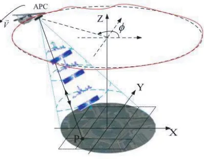
The CSAR imaging geometry is shown in Figure 1. The radar moves in a circular motion in the plane with height H on the platform, and its radius of motion is Rgc. The location of radar in space is

(xa, ya, za) = (Rgccosθ, Rgcsinθ, H), andθ∈(0,2π) represents a certain slow time point. According to

the imaging geometry, the observation scene is a circular area with a radius ofR0; the distance between

the radar and the scene center is Rc =

R2

gc+H2; and the radar pitch angle is θz = arctan(_RH_gc). Assume that the LFM signal transmitted by radar is:

st(t) =ej2π(fct+12γt2) ₍₁₎ The echo signal can be expressed as:

sr(t) =ej2π[fc(t−τ)+12γ(t−τ)2] ₍₂₎ whereτ is the time delay, which can be expressed as:

τ = 2Rp(θ)

c (3)

where Rp(θ) is the distance from the radar to the target. Considering the variation of the radar

platform’s position along with the delay time, Rp(θ) can be expressed as:

RP(θ) =

(3)

Radar moving trace

Detecting area 0 H

R

gc

0 c

R

Figure 1. The geometry of the FMCW CSAR imaging.

3. FMCW CSAR ECHO MODEL WITH MOTION ERROR BASED ON PARAMETRIC SPARSE REPRESENTATION

It is difficult for circular SAR to maintain ideal uniform circular motion in the actual motion process, which results in low-resolution of the image. What’s worse, it may make the echo data unable to focus imaging [14]. Therefore, it is necessary to analyze the impact of nonuniform circular motion on imaging. The geometry of CSAR imaging with motion errors is shown in Figure 2. Because the radar platform moves around the target in a circle, the motion error is composed of the radial motion error and the motion error in the direction of motion [9]. In most studies, a lot of analysis has been done for radial motion errors, and the nonuniform errors in the direction of motion are solved by resampling in azimuth directions or multiple tracks. However, in practice, this method increases the amount of data processed and affects the real-time performance. On the other hand, this method cannot be effective for single track FMCW CSAR. Therefore, it is necessary to analyze and correct the nonuniform circular motion in the direction of motion for single track FMCW CSAR in order to improve the imaging resolution.

(4)

According to the echo signal model of uniform circular motion, the FMCW CSAR imaging echo model of nonuniform circular motion is given. In order to facilitate the analysis, it is assumed that the scattering coeﬃcient of the target isσ(x, y), and FMCW CSAR receives the diﬀerence frequency signal of the echo as follows:

sif(t, θ) =σ(x, y)s∗t(t, θ)·sr(t, θ) =σ(x, y)e−j2π(fcτ+γτ t−12γτ2) (5) The third term is the residual video phase, which is the second term of delay and has little inﬂuence on the phase, so it is usually neglected. Then Fourier transform for fast time to Eq. (5) is:

sif(f, θ) =σ(x, y) exp

−j4πfR_cp(θ)

(6)

The instantaneous frequency is f = γt+fc, and the wave number is k = 2πf/c, then the diﬀerence

echo model can be expressed as:

sif(k, θ) =σ(x, y) exp(−j2kRp(θ)) (7)

Among θ=ωt+1₂awt2,ω is the initial angular velocity, andaw is the angular acceleration. Then Eq. (7) can be discretized into:

S(m, n) =

Dx x=1 Dy y=1

σxyexp(−j2kmRxy(n)) (8)

Dx×Dy is the number of meshes in the imaging scene, andS(m, n) is the echo signal in the mth

frequency and the nth azimuth direction. When noise is considered, the echo signal can be expressed as:

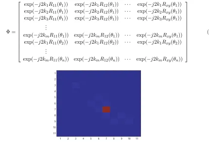
S =σΦ +N (9)

S is the echo data obtained by compressing the distance of the echo signal, andN is the Gaussian noise. The measurement matrix Φ is as follows:

Φ = ⎡ ⎢ ⎢ ⎢ ⎢ ⎢ ⎢ ⎢ ⎢ ⎢ ⎢ ⎢ ⎢ ⎢ ⎣

exp(−j2k1R11(θ1)) exp(−j2k1R12(θ1)) · · · exp(−j2k1Rxy(θ1))

.. .

exp(−j2kmR11(θ1)) exp(−j2kmR12(θ1)) · · · exp(−j2kmRxy(θ1))

.. .

exp(−j2kmR11(θn)) exp(−j2kmR12(θn)) · · · exp(−j2kmRxy(θn)) ⎤ ⎥ ⎥ ⎥ ⎥ ⎥ ⎥ ⎥ ⎥ ⎥ ⎥ ⎥ ⎥ ⎥ ⎦ (10)

(5)

Expression (9) shows that scattering points of the target can be recovered by using the compressed sensing imaging algorithm with known measurement matrix. At this time, the number of sampling points (mn < xy) is declined, which increases the operational eﬃciency. However, when the radar platform uniformly accelerates the circumferential motion, the target range unit will be broadened as shown in Figure 3. Further processing is needed to achieve high resolution imaging. However, the existing motion compensation methods for linear SAR are not applicable in FMCW CSAR imaging due to the complete coupling of azimuth and range directions. Therefore, a new imaging method is necessary to correct motion errors. According to the echo model with motion error, the main error in the direction of motion is that the azimuth uniform sampling caused by initial velocity and angular acceleration is no longer uniform but sparse. Therefore, if the initial velocity and acceleration are estimated, the measure matrix can be obtained. Then the compressed sensing imaging algorithm is used to compensate the error caused by nonuniform circular motion in the motion direction of FMCW CSAR.

4. ESTIMATION OF MOTION ERROR PARAMETERS

In order to eliminate the impact caused by uniformly accelerated motion, the angular acceleration and initial velocity need to be estimated ﬁrstly to reconstruct the measure matrix in the compressed sensing algorithm. According to the parameter in the measure matrix, the least squares method and gradient descent method are applied to estimate the motion parameter.

4.1. Least Squares Method Parameter Estimation

The compressed sensing imaging algorithm is applied to focus image, so the OMP (orthogonal matching pursuit) algorithm is used to reconstruct the target location. The optimal reconstruction expression can be expressed as follows [18, 19]:

σ(p) _{= arg min}

σ σ1+α

S−Φ

w(p)_{, a}(p)

w

σ2

2 (11)

α > 0 is the regularization parameter that balances the recovery error and the sparsity of the solution. In order to eﬀectively estimate the motion parameters containing motion errors, Eq. (11) can be written as follows:

w(p+1)_{, a}(p+1)

w

= arg min

w, aw

S−Φ(w, aw)σ(p)

2 (12)

According to the measure matrix Φ(w, aw), its ﬁrst order Taylor expansion is available:

Φ(w, aw)≈Φ

w(p)_{, a}(p)

w

+ ∂Φ ∂w

w=w(p)

aw=a(wp)

·Δw+ ∂Φ ∂aw

w=w(p)

aw=a(wp)

·Δaw (13)

The projection of the oblique distance on the ground plane in [11] can be expressed as:

R=Rgc−xpcosθ1−ypsinθ1 (14)

Then the slant distance of radar range target can be expressed as: R1 =

R2₊_H2 ₍₁₅₎

According to the measure matrix, its partial derivative can be shown as:

Φm,1 = ⎛ ⎜ ⎜ ⎜ ⎜ ⎜ ⎝

.. .

exp(−j2kmR11(θ1)) exp(−j2kmR12(θ1)) · · · exp(−j2kmRxy(θ1)) ⎞ ⎟ ⎟ ⎟ ⎟ ⎟ ⎠

∂Φm,1

∂w = Φm,1

−j2km2R_Rxy

1

Rg+xpsin

wt1+

1 2awt

2 1

t1−ypcos

wt1+

1 2awt

2 1 t1 (16)

∂Φm,1

∂aw = Φm,1

−j2km2R_Rxy

1

Rgc+xpsinwt1+awt21 1

2t

2

1−ypcos

wt1+

1 2awt

(6)

Then

∂Φ ∂w =

∂Φm,1

∂w , ∂Φm,2

∂w ... ∂Φm,n

∂w

T

(18)

∂Φ ∂aw =

∂Φm,1

∂aw ,

∂Φm,2

∂aw ...

∂Φm,n

∂aw

T

(19)

Assume A(p) = ∂_∂wΦ_w₌_w(p)

aw=a(wp)

,B(p)= _∂a∂Φ_w_w₌_w(p)

aw=a(wp)

. Then

Λ(p) = A(p)σ(p) (20)

Γ(p) = B(p)σ(p) (21)

Therefore, the optimization conditions can be rewritten as follows:

Δw(p),Δa(_wp)

= arg min

Δw,Δaw S−Φ

w(p)_{, a}(p)

w

σ(p)₋_Λ(p)_Δ_w₋_Γ(p)_Δ_a

w

2 (22)

Assume

C(p) ₌

real(Λ(p)) real(Γ(p)) imag(Λ(p)₎ _imag(Γ(p)₎

(23)

D(p) ₌ ⎡ ⎣ real

S−Φ

w(p)_{, a}(p)

w

σ(p)

imag

S−Φ

w(p)_{, a}(p)

w

σ(p) ⎤

⎦_. (24)

Then

Δw(p)

Δa(p)

=

C(p)T_C(p) ₋1

C(p)T _D(p) ₍₂₅₎

The expressions for estimating initial velocity and angular acceleration are as follows:

w(p+1) ₌ _w(p)_{+ Δ}_w(p) ₍₂₆₎

a(p+1)

w = a(wp)+ Δa(wp) (27)

To solve the iteration, more attention should be paid to setting good convergence conditions, that is, when the incremental interval between velocity and angular acceleration is less than a certain error value, we think that it is convergence. Then the measure matrix can be obtained, and the imaging algorithm is applied to focus image.

4.2. Gradient Descent Method Parameter Estimation

In the parameter estimation of least squares method, the inverse matrix needs to be solved by least squares method. When the echo data amount is large, the real-time performance of calculation is seriously aﬀected. Although gradient descent method needs data iteration to realize parameter optimization estimation, the real-time performance of calculation is faster than that of least squares method when the amount of data is large [20]. Therefore, gradient descent method is considered as one of the methods to estimate the motion error.

Formula (22) is equivalent to

Δw(p),Δa(_wp)

= arg min

Δw,Δaw S−Φ

w(p)_{, a}(p)

w

σ(p)₋_Λ(p)_Δ_w₋_Γ(p)_Δ_a

w

2

2 (28)

Assuming Ψ =S−Φ(w(p), a(wp))σ(p), Π = [ Λ(p) Γ(p)] , X = [ _ΔΔ_aw

w ].

The optimization expression can then be expressed as:

Δw(p),Δa(_wp)

= arg min

Δw,Δaw

(7)

So the optimal expression is expressed as an equivalent matrix [20].

Δw(p)_,_Δa(p)

w

= arg min

Δw,Δaw

1 2

Π(p)X(p)−Ψ(p)

T

(Π(p)X(p)−Ψ(p)) (30)

Assume

J = 1 2

Π(p)X(p)−Ψ(p)

T

Π(p)X(p)−Ψ(p)

. (31)

According to the principle of gradient descent method, it can be concluded that: ∂J(p)

∂X(p) = Π

(p)T _Π(p)_X(p)₋_Ψ(p) ₍₃₂₎

Set the step size toβ, then the updated formula for X is as follows:

X(p+1) = X(p)−β∂J

(p)

∂X(p) (33)

The expressions for estimating initial velocity and angular acceleration are as follows:

w(p+1) ₌ _w(p)_{+ Δ}_w(p) ₍₃₄₎

a(p+1)

w = a(wp)+ Δa(wp) (35)

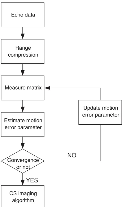
Similarly, in the iteration process, when the incremental interval between velocity and angular acceleration is less than a certain error value, it is considered to converge and stop iteration. Comparing the two parameter estimation algorithms, the gradient descent method avoids the inverse process of large matrix when the echo data is large and improves the eﬃciency of the algorithm. A ﬂowchart of the algorithm is shown in Figure 4.

YES

NO

Echo data

Range compression

Measure matrix

Estimate motion error parameter

Convergence or not

CS imaging algorithm

Update motion error parameter

(8)

4.3. Analysis of Computational Complexity

The main computational burden of the least squares method parameter estimation is from the updating of the OMP algorithm. The independent implementation of OMP costs O(ItM2NK) ﬂoating point

operations, whereIt is the number of iterations and K the sparsity. The computational complexity of the gradient descent method lies on the step size. When the step size is large, it has small amount of calculation, but it may be unconvergent. When the step size is small, it has large amount of calculation, but it may increase the imaging resolution. So it is hard to quantitatively compare the algorithm computational complexities. Therefore, in the following experiments, we compare the computational complexities of diﬀerent algorithms by recording the running time and status of the convergence.

5. SIMULATION RESULTS

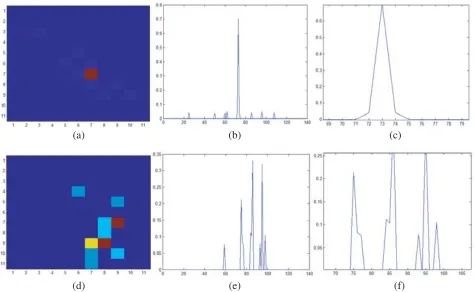
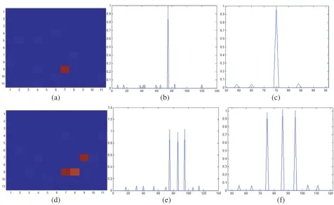
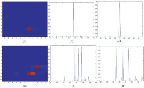
Point targets imaging is simulated to verify the effectiveness of the algorithm. Carrier radar parameters are that the carrier frequency is 10 GHz, flight radius 10 m, flight altitude 10 m, real initial velocity 40 degrees per second with motion error, angular acceleration 3 degrees per second, and the imaging area (−5 m, 5 m). In order to simplify the analysis, the point target located on the ground is selected as the simulation object. Single target coordinates are (1 m, 3 m, 0 m), and multi-target coordinates are (1 m, 3 m, 0 m), (3 m, 2 m, 0 m), (3 m, 1 m, 0 m). The point target imaging with motion errors is shown in Figs. 5(a) and (d). Figs. 5(b), (e), (c), (f) are their range profile and local magnification. Figs. 6(a) and (d) are ideal point target imaging without motion error. Figs. 6(b), (e), (c), (f) are their range profiles. The comparison results show that when the airborne platform does not move uniformly, the target range unit is broadened, and the imaging resolution is reduced. Comparing Fig. 5(a) with Fig. 5(d), it can be seen that the impact of multi-target imaging is more serious. It not only broadens the range unit, but also increases the sidelobes, which further reduces the imaging resolution. Therefore, it is necessary to eliminate the impact of motion errors on single track CSAR. As shown in Fig. 7, the motion error

(a) (b) (c)

(d) (e) (f)

(9)

(a) (b) (c)

(d) (e) (f)

Figure 6. Point target imaging without motion errors.

(a) (b) (c)

(d) (e) (f)

(10)

(a) (b) (c)

(d) (e) (f)

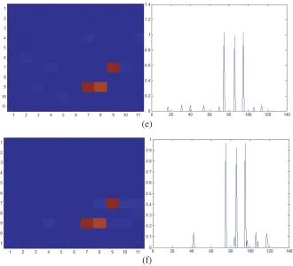
Figure 8. Point target imaging after parametric sparse representation correction by gradient descent method parameter estimation.

is corrected by least squares parameter estimation. Fig. 8 shows the result of motion error corrected imaging which is estimated by gradient descent method. It can be seen that both of the algorithms can correct the widened range unit and reduce the sidelobes caused by the motion error.

Figure 9 shows that the target imaging after Parametric Sparse Representation Correction in diﬀerent methods for various noises. The results tell us that increasing noise causes the resolution of the target imaging to decrease. Both the Gradient descent method and the Least squares parameter estimation can correct the motion error in the direction, but the two methods cannot obtain better results in a low SNR.

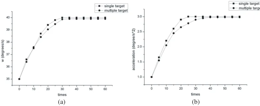
Considering the real-time performance and eﬃciency of the algorithm, the simulation process is analyzed. The initial velocity is 35 degrees per second, and the initial angular acceleration is 1 degree per square second. the iteration process of velocity is shown in in Fig. 10(a), Fig. 11(a), and the iteration process of angular acceleration is shown in Fig. 10(b), Fig. 11(b). The results of Fig. 10 show the velocity converge at 30 times for single target and 40 times for multiple targets, and the angular acceleration converge at 30 times and 35 times for multiple targets by least square method. The results of Fig. 11 show that the velocity converges at 30 times for single target and 30 times for multiple targets, and the angular acceleration converges at 25 times and 35 times for multiple targets by gradient descent method.

By comparing the convergence of the two parameters, it can be seen that the convergence rate of the algorithm can meet the real-time requirement when iterating about 30 times for a single objective and about 40 times for multi-objectives. At the same time, compared with the two methods, for single target both of the methods can correct the error, and the rates of convergence are similar. For multiple targets, the convergence of gradient descent method is more quickly.

The convergence processes in diﬀerent SNRs are simulated, and the results are shown in Fig. 12. From the results, the convergence times vary from the SNR, and the lower the SNR is, the more the convergence times are. Both of the methods satisfy the situation.

(11)

(a)

(b)

(c)

(12)

(e)

(f)

Figure 9. Point target imaging after parametric sparse representation correction in diﬀerent methods for various noise. (a) SNR =−10 point target imaging after parametric sparse representation correction by least squares parameter estimation. (b) SNR = −10 point target imaging after parametric sparse representation correction by gradient descent method parameter estimation. (c) SNR =−5 point target imaging after parametric sparse representation correction by least squares parameter estimation. (d) SNR = −5 point target imaging after parametric sparse representation correction by gradient descent method parameter estimation. (e) SNR = 0 point target imaging after parametric sparse representation correction by least squares parameter estimation. (f) SNR = 0 point target imaging after parametric sparse representation correction by gradient descent method parameter estimation.

(a) (b)

(13)

(a) (b)

Figure 11. The relationship between the number of iterations and the convergence of error parameters in Gradient descent method. (a) Convergence process of angular initial velocity. (b) Convergence process of angular acceleration.

(a) (b)

Figure 12. The convergence processes in diﬀerent SNRs. (a) Convergence process of angular initial velocity. (b) Convergence process of angular acceleration.

(14)

(c)

Figure 13. Parametric representation of measured data before and after correction of motion errors. (a) Before correction of motion errors, (b) after correction of motion errors estimated by Least squares method, (c) after correction of motion errors estimated by Gradient descent method.

algorithm. When the initial angular velocity and acceleration are unknown in the measured data, motion parameters are estimated by the least squares method and gradient descent method, and the measure matrix is obtained. Then the final image can be obtained by imaging algorithm. By comparing the images before and after the parametric sparse representation compensation, we can see that the imaging resolution of the target has been improved, and especially the sidelobe has been effectively suppressed in the range of red boxes in Figs. 13(a), 13(b), and 13(c). The simulations show that the PSLR (Peak side lobe ratio) of picture (b) is−2.4253 dB, and the PSLR of picture (c) is−3.8709 dB, which demonstrates the effectiveness of the proposed algorithm.

6. CONCLUSION

Single-track FMCW CSAR is affected by external factors during its practical application, which results in its nonuniform circular motion. The image resolution reduction caused by nonuniform circular motion is simulated. In order to avoid such problems, the parametric sparse representation based on compressed sensing imaging algorithm is proposed to correct motion errors. Besides, the least squares method and gradient descent method are introduced to estimate motion error parameters. Simulations are conducted to verify the algorithm effective. The simulation results show that the method can effectively correct the range cell broadening and sidelobe increase caused by nonuniform circular motion to improve the imaging resolution. The error in the direction of motion and radial error will be combined to analyze by parameters estimation and improve the imaging resolution in the future work.

REFERENCES

1. Cumming, I. G. and F. H. Wong,Digital Processing of Synthetic Aperture Radar Data: Algorithms and Implementation, Artech House, Norwood, MA, USA, 2005.

2. Tang, S., et al., “Processing of monostatic SAR data with general conﬁgurations,” IEEE Trans. Geosci. Remote Sens., Vol. 12, No. 53, 6529–6546, 2015.

3. Prats-Iraola, P., et al., “On the processing of very high resolution spaceborne SAR data,” IEEE Trans. Geosci. Remote Sens., Vol. 10, No. 52, 6003–6016, 2014.

(15)

5. Moreira, A., P. Prats-Iraola, M. Younis, G. Krieger, I. Hajnsek, and K. P. Papathanassiou, “A tutorial on synthetic aperture radar,”IEEE Geosci. Remote Sens., Vol. 3, No. 1, 6–43, 2013. 6. Ciuonzo, D., G. Romano, and R. Solimene, “Performance analysis of time-reversal MUSIC,”IEEE

Transactions on Signal Processing, Vol. 63, No. 10, 2650–2662, 2015.

7. Ciuonzo, D., “On time-reversal imaging by statistical testing,” IEEE Transactions on Signal Processing Letters, Vol. 24, No. 4, 1024–1028, 2017.

8. Ciuonzo, D., V. Carotenuto, and A. De Maio, “On multiple covariance equality testing with application to SAR change detection,” IEEE Transactions on Signal Processing, Vol. 65, No. 19, 5078–5091, 2017.

9. Soumekh, M., “Reconnaissance with slant plane circular SAR imaging,” IEEE Transactions on Image Processing, Vol. 5, No. 8, 1252–1265, 1996.

10. Soumekh, M.,Synthetic Aperture Radar Signal Processing with MATLAB Algorithms, Wiley, New York, 1999.

11. Ao, D., R. Wang, C. Hu, and Y. Li, “A sparse SAR imaging method based on multiple measurement vectors model,”Remote Sens., Vol. 9, No. 297, 1–22, 2017.

12. Jia, G., W. Chang, Q. Zhang, and X. Luan, “The analysis and realization of motion compensation for circular synthetic aperture radar data,” IEEE Journal of Selected Topics in Applied Earth Observations and Remote Sensing, Vol. 9, No. 4, 3060–3071, 2016.

13. Guo, Z. Y., Y. Lin, W. X. Tan, Y. P. Wang, and W. Hong, “Circular SAR motion compensation using trilateration and phase correction,”IET International Radar Conference, 1–6, 2013.

14. Xie, H., S. Shi, D. An, et al., “Fast factorized backprojection algorithm for one-stationary bistatic spotlight circular SAR image formation,” IEEE Journal of Selected Topics in Applied Earth Observations and Remote Sensing, Vol. 10, No. 4, 1494–1510, 2017.

15. Zhang, B., X. Zhang, and S. Wei, “A circular SAR image autofocus algorithm based on minimum entropy,”2015 IEEE 5th Asia-Pacific Conference on Synthetic Aperture Radar (APSAR), 152–155, 2015.

16. Lin, Y., W. Hong, and W. Tan, “Compressed sensing technique for circular SAR imaging,” 2009 IET International Radar Conference, 1–4, 2009.

17. Wang, X., B. Deng, H. Wang, and Y. Qi, “Ground moving target imaging based on motion compensation for circular SAR,” 2017 9th International Conference on Advanced Infocomm Technology, 372–377, 2017.

18. Chen, Y.-C., G. Li, Q. Zhang, Q.-J. Zhang, and X.-G. Xia, “Motion compensation for airborne SAR via parametric sparse representation,” IEEE Trans. Geosci. Remote Sens., Vol. 55, No. 1, 551–561, 2017.

19. Rao, W., G. Li, X. Wang, and X.-G. Xia, “Parametric sparse representation method for ISAR imaging of rotating targets,” IEEE Trans. Aerosp. Electron. Syst., Vol. 2, No. 50, 910–919, 2014. 20. Li, X., S. Liu, and W. Xie, “A novel conjugate gradient method for sensing matrix optimization