Coordination of Frequency and Load Resistor to Improve Efficiency
of Wireless Power Transfer System Under Frequency Drift
Zhongqi Li1, 2, Wangyang Cheng1, Jiliang Yi1, *, and Junjun Li1
Abstract—Magnetic resonant wireless power transfer (WPT) is an emerging technology that may create new applications for wireless power charging. However, low efficiency resulting from resonant frequency drift is a main obstructing factor for promoting this technology. In this paper, a novel method of coordinating the operating frequency and load resistor is proposed to prevent frequency drift. The system efficiency and input impedance are obtained by solving the system equivalent equations. In addition, the new resonant frequencies can be obtained by solving the input impedance equations. Moreover, the process of the coordination method is illustrated. When resonant frequency drift occurs, the system can now operate at the resonant state, and the efficiency can be improved by using the proposed method. The WPT system via magnetic resonance coupling is designed. Simulated and experimental results validating the proposed method are given.
1. INTRODUCTION
Wireless power transfer (WPT) methods are receiving increasing attention in the international research community [1, 2]. A new wireless power transfer technology based on strongly coupled magnetic resonances is proposed [3–5]. This technology is used widely in the fields of medical devices, charging of mobile and electric vehicles [6–8]. One of the most important problems is to improve efficiency in magnetic resonant wireless power transfer system [3–5].
There are many researches in the WPT system in order to obtain high transfer efficiency. The first approach is to optimize the circuit topologies [9–11]. The circuit topological structure of the series-shunt mixed-resonant is proposed to obtain high efficiency [9]. The second approach is to use novel system structures, such as a three-coil structure [12–14], a novel four-coil structure and a multiple-coil structure [15–18]. The third approach is to optimize the parameters of resonant coil [19, 20]. Finally, the optimization methods are used to improve the efficiency, such as optimizing the operating frequency [21], optimizing coupling coefficients [22, 23] and the impedance matching method [24–27]. However, these methods are analyzed in the WPT system under the condition of working at the resonant state.
The condition of working at the resonant state is rather difficult to be satisfied in practical applications because some reasons may result in the resonant frequency drift as follows: (1) inductance or capacitance of the coil may change easily affected by external environment changes, and resonant frequency drift will then occur; (2) Some materials (such as aluminum foil, styrofoam, and humans) may alter the inductance or capacitance of the resonant coil [3], and resonant frequency drift may occur; (3) The error between the nominal value of the capacitor and the actual value of the capacitor may result in resonant frequency drift; (4) the capacitance of the resonant coil may be changed with the variations of temperature, the resonant frequency is also changed as the the capacitance of the resonant coil is changed. The efficiency will drastically decrease when resonant frequency drift occurs. In order to
Received 15 October 2018, Accepted 21 November 2018, Scheduled 3 December 2018 * Corresponding author: Jiliang Yi (ieee [email protected]).
maintain the required resonant state, the resonant frequency of each coil is adjusted manually by using the external compensating capacitance when the external environment is changed. However, the WPT system may have several resonant coils in practical applications [28]. It is impractical for the WPT system to manually adjust the external compensating capacitance of each coil in practical applications. A frequency-tuned wireless charging system is proposed and successfully demonstrated to enhance the power transfer efficiency [26]. However, it is not considered that the resonant frequencies are changed with the load resistor variations. In this paper, a method of coordinating the operating frequency and load resistor is proposed. It is found that there may be multiple resonant frequencies for different load resistors. The efficiency is the highest at the optimum resonant frequency. When resonant frequency drift occurs, the optimum resonant frequency may be obtained by using the proposed method. Then the system may operate at the resonant state and the optimum efficiency may be obtained.
The rest of the paper is organized as follows. Section 2 establishes the system model and theory. Section 3 analyzes the efficiency with only adjusting the operating frequency. Section 4 analyzes the proposed efficiency improvement method. Section 5 presents the experimental setup and measurement results. Section 6 concludes this paper.
2. MODEL AND THEORETICAL ANALYSIS
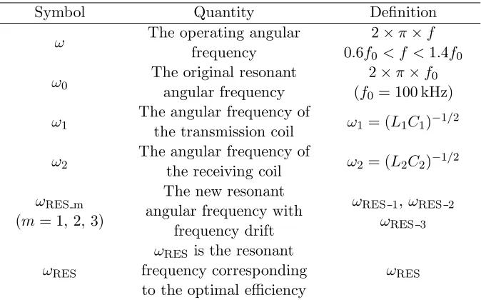
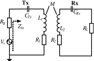
The WPT system is composed of two resonant coils: transmission and receiving resonant coils, labeled as Tx and Rx, as shown in Fig. 1. Dis the distance between Tx and Rx,CTxthe external compensating capacitance of Tx, and CRx the external compensating capacitance of Rx. The WPT system can be represented in terms of lumped circuit elements (L, C, and R), as shown in Fig. 2. Vs is the source power, R1 the parasitic resistor of Tx, R2 the parasitic resistor of Rx, Rs the internal resistor of the power source, RL the load resistor, L1 the inductance of Tx, L2 the inductance of Rx, M the mutual inductance between Tx and Rx,Zinthe input impedance,ω1the angular frequency of Tx,ω2the angular frequency of Rx, and ω0 the original resonant angular frequency of each coil. All angular frequencies are shown in Table 1.
Table 1. Angular frequencies.
Symbol Quantity Definition
ω The operating angular
frequency
2×π×f 0.6f0 < f <1.4f0
ω0
The original resonant angular frequency
2×π×f0 (f0 = 100 kHz)
ω1
The angular frequency of
the transmission coil ω1 = (L1C1)− 1/2
ω2
The angular frequency of
the receiving coil ω2 = (L2C2)− 1/2
ωRES m (m= 1, 2, 3)
The new resonant angular frequency with
frequency drift
ωRES 1,ωRES 2
ωRES 3
ωRES
ωRES is the resonant frequency corresponding to the optimal efficiency
ωRES
By applying Kirchhoff’s voltage law (KVL), the WPT system is presented as follows:
Z1I1+jωMI2 =Vs
jωMI1+Z2I2 = 0 (1)
Z1 =RS+R1+jωL1+ 1/(jωCT x)
Load D CTx power Tx CRx Rx
Figure 1. The simplified schematic of the WPT system based on magnetically coupling resonator.
M
Vs
Rs
CTx L 1 R1 CRx L2 R2 RL Tx Rx Zin
Figure 2. The equivalent circuit model for the WPT system. Each coil is modeled as series resonators.
whereI1 is the current of Tx, I2 the current of Rx, and ω the operating angular frequency. The expressions ofI1 and I2 can be obtained by solving Eqs. (1) and (2).
⎧ ⎪ ⎪ ⎨ ⎪ ⎪ ⎩
I1 = VsZ 2
Z1Z2+ (ωM)2
I2 =−Z jωMVs 1Z2+ (ωM)2
(3)
The expression of efficiency in Eq. (4) is as follows:
η=I 2 2RL
VsI1
= (ωM) 2R
L
Z1Z22+ (ωM)2Z2
(4)
Equation (2) is substituted into Equation (4). Then the expression of efficiency in Equation (5) can be obtained.
η=I 2 2RL
VsI1
= U
2U L
{(1 +Us+jε1Q1)(1 +UL+jε2Q2)2+ (1 +UL+jε2Q2)U2}
(5)
where the source matching factor is defined as Us = Rs/R1, the load matching factor defined as
UL=RL/R2, the strong-coupling parameter defined as U =ωM/(R1R2)1/2, the unload quality factor of Tx defined as Q1 =ωL1/R1, the unload quality factor of Rx defined as Q2 =ωL2/R2, the angular frequency deviation factor of Tx defined asξ1 = 1−ω21/ω2, and the angular frequency deviation factor of Rx defined asξ2 = 1−ω22/ω2.
The input impedance can be defined by Eq. (6)
Zin=Vs/I1−Rs (6)
Equation (2) is substituted into Eq. (6). Then the expression of the input impedance can be obtained as follows:
Zin = R1
[(U2+(1+Us)(1+UL)−Q1Q2ε1ε2)+j(Q1ε1(1+UL) +Q2ε2(1 +Us))]((1 +UL)−jQ2ε2) (1 +UL)2+Q2
2ε22
−Rs (7)
Equation (7) can be simplified into Eq. (8)
Zin=R1
[(1 +UL)2+U2(1 +UL) +Q22ε22] +j[(1 +UL)2Q1ε1+Q1ε1Q22ε22−U2Q22ε22] (1 +UL)2+Q2
2ε22
(8)
According to Eq. (8), the input impedance characteristic angle (θ) between Vs and I1 can be obtained as follows:
θ = arctan(Im(Zin)/Re(Zin))
= arctan
(1 +UL)2Q1ε1+Q1Q22ε1ε22−U2Q2ε2 (1 +UL)2+U2(1 +U
L) +Q22ε22
where Re(Zin) is the real component of Zin, and Im(Zin) is the imaginary component of Zin. θ is the input impedance characteristic angle. Whenθ= 0, the impedance is purely resistive, and Eq. (10) can be obtained from Eq. (9).
L1L22−L2M2
ω6+(R
2+RL)2L1−2L1L22ω22−L1L22ω12+L2M2ω22
ω4 +L1L22ω42+ 2L1L22ω12ω22−(R2+RL)2L1ω21
ω2−L
1L22ω12ω24= 0 (10) The resonant angular frequencies can be obtained by solving Eq. (10). The resonant angular frequencies ωRES m (m= 1,2,3) are dependent on the angular frequency of the transmission resonant coil ω1, the angular frequency of the receiving resonant coil ω2, and the load resistor RL when the parameters of each resonant coil and the transfer distance D are given. According to Eq. (5), the efficiency is also dependent on the resonant angular frequencies ωRES m and the load resistorRL.
3. ANALYSIS OF ADJUSTING FREQUENCY METHOD
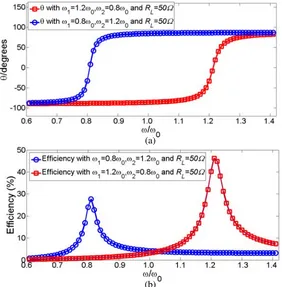
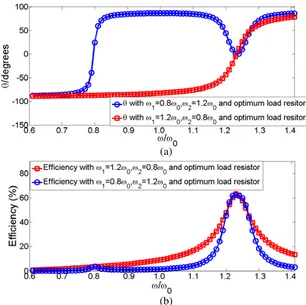
In this section, the efficiency can be improved by using the method of adjusting the operating frequency. When resonant frequency drift occurs and the load resistor is fixed at 50 Ω, according to (9),θbecomes greater than zero atω=ω0and the efficiency is reduced according to Eq. (5). Fig. 3(b) shows efficiency versus ω/ω0 profiles for different combinations of ω1 and ω2. It may be observed that the efficiency is 4.1% withω1 = 0.8ω0,ω2 = 1.2ω0, and ω=ω0, and the efficiency is 3.4% withω1= 1.2ω0,ω2= 0.8ω0, and ω =ω0. This has clearly shown that when the resonant frequency of the two resonant coils drifts away (due to e.g., parameters variation), working at the original resonant frequency will no longer result in high efficiency. This is because θ is no longer close to zero degree (close to plus/minus 90 degrees instead) at the original resonant angular frequency, as may be observed from Fig. 3(a). The circuit is no longer resistive, and the energy tends to be stored in the inductance/capacitance instead of being transferred away, resulting in a low power transfer efficiency.
(b) (a)
The WPT system can operate at the resonant state by using the method of adjusting the operating frequency. θ is equal to zero at the new resonant frequency according to Eq. (9). The efficiency is improved according to Eq. (5). It can be seen from Fig. 3(a) that the new resonant angular frequency is 0.80ω0 with ω1 = 0.8ω0, ω2 = 1.2ω0 and RL = 50 Ω; whereas the new resonant angular frequency is 1.20ω0 withω1= 1.2ω0,ω2 = 0.8ω0 and RL= 50 Ω. The efficiency is very low at the original resonant angular frequency, whereas the efficiency can be improved at the new resonant angular frequency. Fig. 3(b) shows efficiency versus ω/ω0 profiles for different combinations of ω1 and ω2. It may be observed that the efficiency is 27.8% with ω= 0.80ω0,ω1= 0.8ω0 and ω2 = 1.2ω0, and the efficiency is 46.8% with ω= 1.20ω0,ω1= 1.2ω0 and ω2 = 0.8ω0.
4. PROPOSED METHOD
4.1. Analysis of the Effects of Frequency and Load Resistor on Efficiencies
The efficiency can be improved by adjusting the operating frequency when the resonant frequency drift occurs. However, the efficiency is still low. For example, the efficiency is 27.8% with ω1 = 0.8ω0,
ω2 = 1.2ω0 and RL = 50 Ω, and the efficiency is 46.8% with ω1 = 1.2ω0, ω2 = 0.8ω0 and RL = 50 Ω. In this section, the method of coordinating the operating angular frequency and the load resistor is proposed in order to further improve efficiency.
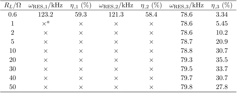
According to Eq. (10), the resonant angular frequencies are related to the angular frequency of the transmission resonant coil ω1, the angular frequency of the receiving resonant coilω2 and the load resistor RL. The efficiency is dependent on the resonant angular frequencies, ω1,ω2 and RL according to Eq. (5). The resonant frequencies can be calculated by using Eq. (10), then the efficiencies can be obtained according to Eq. (5). Table 2 to Table 5 show calculated efficiencies and resonant frequencies for different load resistors, ω1 and ω2. It can be seen that the resonant frequency is changed as the load resistors ω1 and ω2 are changed. The efficiency is also changed as the load resistor and resonant frequencies are changed.
Table 2. Efficiencies and Resonant Frequency withω1= 0.8ω0 and ω2 = 1.2ω0.
RL/Ω ωRES 1/kHz η1 (%) ωRES 2/kHz η2 (%) ωRES 3/kHz η3 (%)
0.6 123.2 59.3 121.3 58.4 78.6 3.34
1 ×a × × × 78.6 5.45
2 × × × × 78.6 10.2
5 × × × × 78.7 20.9
10 × × × × 78.8 30.7
20 × × × × 79.3 35.5
30 × × × × 79.5 33.7
40 × × × × 79.7 30.7
50 × × × × 79.8 27.8
ωRES m(m= 1,2,3) are resonant angular frequencies. ηm(m= 1,2,3) are efficiencies atωRES m (m= 1,2,3), respectively.
a ‘×’ is denoted as no value.
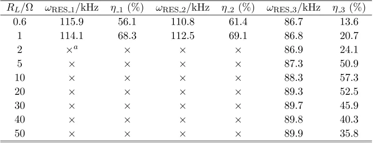
Table 3. Efficiencies and resonant frequency withω1= 0.9ω0 and ω2 = 1.1ω0.
RL/Ω ωRES 1/kHz η1 (%) ωRES 2/kHz η2 (%) ωRES 3/kHz η3 (%)
0.6 115.9 56.1 110.8 61.4 86.7 13.6
1 114.1 68.3 112.5 69.1 86.8 20.7
2 ×a × × × 86.9 24.1
5 × × × × 87.3 50.9
10 × × × × 88.3 57.3
20 × × × × 89.3 52.5
30 × × × × 89.7 45.9
40 × × × × 89.8 40.3
50 × × × × 89.9 35.8
ωRES m(m= 1,2,3) are resonant angular frequencies. ηm(m= 1,2,3) are efficiencies atωRES m(m= 1,2,3),respectively.
a ‘×’ is denoted as no value.
Table 3 shows calculated efficiencies and resonant frequencies with ω1 = 0.9ω0 and ω2 = 1.1ω0. Resonant frequencies are equal to 115.9 kHz, 110.8 kHz, and 86.7 kHz with RL = 0.6 Ω, respectively. Resonant frequencies are equal to 114.1 kHz, 112.5 kHz, and 86.8 kHz with RL = 1 Ω, respectively. However, there is only a resonant frequency for a given load resistor, which is varied from 2 Ω to 50 Ω. It can be seen that the resonant frequency is varied from 86.9 kHz to 89.9 kHz when the load resistor is varied from 2 Ω to 50 Ω. The efficiency is also changed as the load resistor and resonant frequencies are changed. The maximum efficiency is 69.1%, the resonant frequency is equal to 112.5 kHz and the load resistor is 1 Ω at the maximum efficiency point.
Table 4. Efficiencies and resonant frequency withω1= 1.2ω0 and ω2 = 0.8ω0.
RL/Ω Resonant frequencies/kHz η (%)
0.6 125.4 13.7
1 124.2 20.7
2 124.1 33.2
5 124.1 51.6
10 123.4 60.3
20 121.5 60.1
30 120.7 55.3
40 120.4 50.0
50 120.1 46.8
Table 4 shows calculated efficiencies and resonant frequencies with ω1 = 1.2ω0 and ω2 = 0.8ω0. There is only a resonant frequency for a given load resistor, which is varied from 0.6 Ω to 50 Ω. It can be seen that the resonant frequency is varied from 125.4 kHz to 120.1 kHz when the load resistor is varied from 0.6 Ω to 50 Ω. The efficiency is varied from 13.7% to 60.3% when the load resistor is varied from 0.6 Ω to 10 Ω. The efficiency is varied from 60.3% to 46.8% when the load resistor is varied from 10 Ω to 50 Ω.
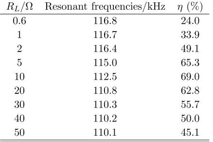
Table 5. Efficiencies and resonant frequency withω1= 1.1ω0 and ω2 = 0.9ω0.
RL/Ω Resonant frequencies/kHz η (%)
0.6 116.8 24.0
1 116.7 33.9
2 116.4 49.1
5 115.0 65.3
10 112.5 69.0
20 110.8 62.8
30 110.3 55.7
40 110.2 50.0
50 110.1 45.1
0.6 Ω to 10 Ω. The efficiency is varied from 69.0% to 45.1% when the load resistor is varied from 10 Ω to 50 Ω.
4.2. Coordinating Frequency and Load Resistor Method
It is noted that the resonant frequency can be changed with load resistor variations, and the efficiency can also be changed with the operating frequency and load resistor variations. Therefore, we propose a method of coordinating the operating frequency and the load resistor to improve efficiency. The process of the proposed coordinating method is as follows:
1) The load resistor is changed from 0.5 Ω to 100 Ω in a step of 0.1 Ω according to the condition of practical constraints. It is assumed that the resonant frequency of each coil is varied from 0.8ω0 to 1.2ω0 when external environment changes [3].
2) The resonant angular frequencies at a given load resistor can be obtained by solving Eq. (10). 3) The resonant angular frequencies at a given load resistor are substituted into Eq. (5). The efficiency at a given resonant angular frequency and load resistor can then be obtained.
4) Compared to the efficiency at a given resonant angular frequency and load resistor, the optimum efficiency is obtained.
5) According to the optimum efficiency, the optimum load resistor and the optimum resonant angular frequency can be obtained. The detailed optimization process is shown in Fig. 4.
Using the proposed method, the simulation results are shown in Fig. 5 and Fig. 6. Fig. 5(a) shows the input impedance characteristic angle (θ) versusω/ω0profiles for different combinations ofω1andω2. It can be seen that resonant angular frequencies are equal to 0.79ω0, 1.22ω0, and 1.23ω0 withω1 = 0.8ω0 and ω2 = 1.2ω0, respectively. And the resonant angular frequency is equal to 1.22ω0 withω1 = 1.2ω0 and ω2= 0.8ω0, respectively. Fig. 6(a) shows the input impedance characteristic angle (θ) versusω/ω0 profiles for different combinations of ω1 and ω2. It can be seen that resonant angular frequencies are equal to 0.87ω0, 1.13ω0, and 1.14ω0 with ω1 = 0.9ω0 and ω2 = 1.1ω0, respectively. And the resonant angular frequency is equal to 1.13ω0 with ω1 = 1.1ω0 and ω2 = 0.9ω0, respectively. Simulation results of the resonant angular frequencies are the same as calculation results of Eq. (10). Fig. 5(b) shows efficiency versus ω/ω0 profiles for different combinations of ω1 and ω2. It may be observed that the efficiency is 63.6% with ω = 1.22ω0, ω1 = 0.8ω0, and ω2 = 1.2ω0 and the efficiency is 63.1% with
ω = 1.23ω0, ω1 = 0.8ω0, and ω2 = 1.2ω0; whereas the efficiency is 4.3% with ω = 0.79ω0, ω1 = 0.8ω0 and ω2 = 1.2ω0, and the efficiency is 63.0% with ω= 1.22ω0,ω1= 1.2ω0, and ω2= 0.8ω0.
Figure 6(b) shows efficiency versus ω/ω0 profiles for different combinations of ω1 and ω2. It may be observed that the efficiency is 69.1% withω= 1.13ω0,ω1 = 0.9ω0 and ω2= 1.1ω0, and the efficiency is 68.3% withω= 1.14ω0,ω1= 0.9ω0 and ω2= 1.1ω0; whereas the efficiency is 20.7% withω= 0.87ω0,
START
Parameter setting: 1, 2, 0, L1, L2,
R1, R2, M (i)> *
END Load resistor setting
RL_Min<RL(i)<RL_Max
RL(i):=RL(i)+0.1
*
= (i) R*=RL(i)
*= (i)
Output the best solution found Calculating the resonant
angular frequency
Calculating efficiencies
RL_Max>RL(i) Yes
No Initialization of the efficiency ( *),
the angular frequency ( ω*), and the load resistor (R*)
Yes
No
η
Ω
ω ω ω
η η
η η
ω ω
Figure 4. Flowchart of the optimization process by coordinating operating frequency and load resistor.
(b) (a)
Figure 5. Simulation results withω1 = 1.2ω0,ω2 = 0.8ω0 andω1 = 0.8ω0 andω2 = 1.2ω0. (a) θversus
(b) (a)
Figure 6. Simulation results with ω1 = 1.1ω0, ω2 = 0.9ω0 and ω1 = 0.9ω0, ω2 = 1.1ω0. (a) θ versus
ω/ω0. (b) Efficiencies versus ω/ω0.
The optimum resonant angular frequency and the optimum efficiency can be obtained by using the proposed method.
5. MEASUREMENT RESULTS
5.1. The Experimental System
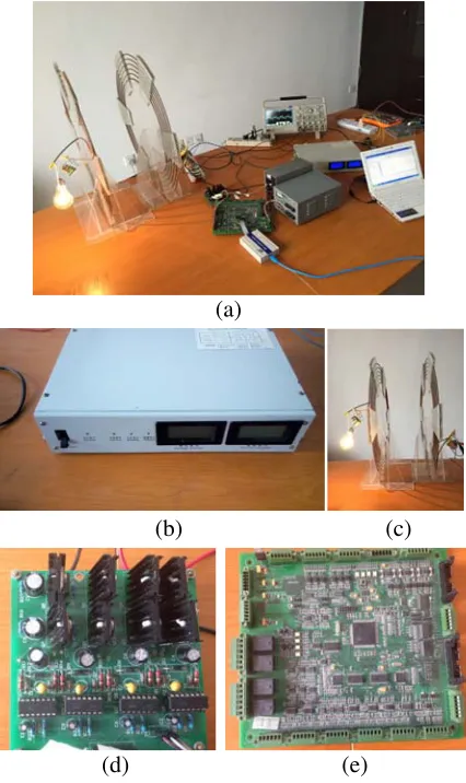
To validate the proposed method, the prototype model of the system has been built, as shown in Fig. 7. It is composed of the DC voltage source, two resonant coils, the quadruple-frequency inverter and the load. The value of the DC voltage source is 15 V, the fabricated DC voltage source is shown in Fig. 7(b). The two resonant coils are transmission and receiving coils. The transmission resonant coil is on the right. The receiving resonant coil is on the left, as shown in Fig. 7(c). The diameter of the transmission resonant coil is 40 cm with a pitch of 2 cm for approximately 6 turns. The parameters of the receiving resonant coil are the same as those of the transmission resonant coil. The parameters of the resonant coils can be calculated by using [29, 30]. An impedance analyzer TH2829A is used to extract the parameters in Eqs. (1) and (2). The original resonant frequency is set to be 100 kHz. The parameters of the resonant coils are listed in Table 6.
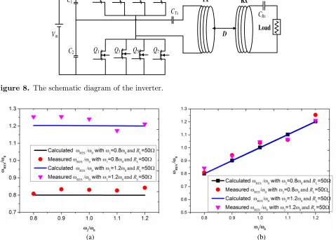
The quadruple-frequency inverter is used in this paper. Fig. 8 shows the schematic diagram of the inverter. The inverter consists of eight switch MOSFETs (Q1∼Q8) and two electrolytic capacitors (C1 and C2). IR2110 and IRF3205 are used as the gate driver and the switch MOSFET. The fabricated inverter is shown in Fig. 7(d). The inverter is controlled by the pulse-width-modulation (PWM) signals from the DXP28335 controller, as shown in Fig. 7(e). The inverter is suitable for working at high frequency (100 kHz–1 MHz).
Table 6. Parameters of the resonant coils.
Symbol Quantity Value
L1 the inductance of Tx 29.70µH
L2 the inductance of Rx 29.70µH
C1 the external compensating capacitance of Tx 85.28 nF
C2 the external compensating capacitance of Rx 85.28 nF
R1 the resistor of Tx 0.30 Ω
R2 the resistor of Rx 0.29 Ω
f0 the original resonant frequency 100.0 kHz
(b) (a)
(d)
(c)
(e)
Figure 7. The experimental setup of the WPT system. (a) The overall experimental setup. (b) The DC voltage source. (c) The resonant coils. (d) The quadruple-frequency inverter. (e) The DXP28335 controller.
5.2. Adjusting the Operating Frequency
After replacing the bulb with a resistor, we firstly measure the system resonant frequencies and efficiencies by adjusting the operating frequency method. Fig. 9(a) shows the calculated and measured
Vin
C1
C2 Q1
Q2
Q3
Q4
Q5
Q6
Q7
Q8
CTx C
Rx
Load
D
Tx Rx
Figure 8. The schematic diagram of the inverter.
(b) (a)
Figure 9. Measured and calculated results ofωRES/ω0, (a)ωRES/ω0 versusω2/ω0 for differentω1 with
RL= 50 Ω. (b) ωRES/ω0 versusω1/ω0 for different ω2 with RL= 50 Ω.
(b) (a)
Figure 10. Measured and calculated results of efficiencies, (a) Efficiencies versus ω1/ω0 for different
the following ωRES is also the resonant angular frequency at the maximum efficiency point). It can be seen that ωRES/ω0 is nearly constant as the ω2/ω0 is varied from 0.8 to 1.2. ωRES/ω0 is nearly equal to 1.2 with ω1 = 1.2ω0 and RL = 50 Ω; whereas ωRES/ω0 is nearly equal to 0.8 with ω1 = 0.8ω0 and
RL= 50 Ω.
Figure 9(b) shows the calculated and measuredωRES/ω0profiles for differentω2. It can be seen that
ωRES/ω0 is changed along with the change of ω1/ω0. It is found that the resonant angular frequency
ωRES is determined by ω1 withRL= 50 Ω. This is because the input impedance characteristic angle is equal to zero at ω=ω1 in term of Eq. (9) even though the frequency of Rx deviates from the original resonant frequency. Fig. 10(a) shows the calculated and measured efficiencies versus ω1/ω0 profiles for different ω2. The efficiency is varied from 34.7% to 51.2% at ω2 = 0.8ω0 when ω1/ω0 is changed from 0.8 to 1.2. The efficiency is varied from 31.7% to 48.7% atω2 = 1.2ω0 whenω1/ω0 is changed from 0.8 to 1.2. Fig. 10(b) shows the calculated and measured efficiencies versus ω2/ω0 profiles for different ω1. The efficiency is nearly constant for different ω1 as ω2/ω0 is changed from 0.8 to 1.2. The efficiency is nearly equal to 32% atω1 = 0.8ω0; whereas the efficiency is nearly equal to 49% atω1 = 1.2ω0.
5.3. The Proposed Method
When the proposed method is used, Fig. 11(a) shows the calculated and measured optimum RL versus
ω2/ω0 profiles for differentω1. It can be seen that optimumRL is changed as ω2/ω0 is varied.
(b) (a)
Figure 11. Measured and calculated results of optimumRL, (a) OptimumRLversusω2/ω0for different
ω1. (b) Optimum RL versusω1/ω0 for different ω2.
Figure 11(b) shows the calculated and measured optimum RL versus ω1/ω0 profiles for different
ω2. It can also be seen that optimum RL is also changed as ω1/ω0 is varied. There exists an optimum
RL for different combinations of ω,ω1, and ω2 in order to obtain the optimum efficiency.
Figure 12(a) shows the calculated and measured optimumωRES/ω0versusω2/ω0profiles for different
ω1. The optimumωRESis changed at ω1 = 0.8ω0 along with the change ofω2 asω2/ω0 is changed from 0.8 to 1.2; whereas the optimumωRESis nearly constant and equal to 1.2ω0 withω1 = 1.2ω0 asω2/ω0is changed from 0.8 to 1.2. Fig. 12(b) shows the calculated and measured optimumωRES/ω0 versusω1/ω0 profiles for different ω2. The optimum ωRES is changed at ω2 = 0.8ω0 as ω1/ω0 is changed; whereas the optimum ωRES is nearly constant withω2 = 1.2ω0 as ω1/ω0 is changed from 0.8 to 1.2. It can be seen that ωRES is changed along with the change of ω1 when the method of adjusting the operating frequency is used, whereas the optimum ωRES is determined by ω1,ω2 and the optimum load resistor
(b) (a)
Figure 12. Measured and calculated results of optimumωRES/ω0, (a) OptimumωRES/ω0 versusω2/ω0 for different ω1 with optimum RL. (b) OptimumωRES/ω0 versus ω1/ω0 for different ω2 with optimum
RL.
When the optimum ωRES and optimum load resistor are used, Fig. 13(a) shows the calculated and measured efficiencies versusω2/ω0 profiles for differentω1. The efficiency is varied from 68.9% to 62.5% with ω1 = 0.8ω0 as ω2/ω0 is changed from 0.8 to 1.2. The efficiency is varied from 64.2% to 71.8% with ω1 = 1.2ω0 as ω2/ω0 is changed from 0.8 to 1.2. Fig. 13(b) shows the calculated and measured efficiencies versus ω1/ω0 profiles for different ω2. The minimum efficiency is 64.2% with ω1 = 0.8ω0 as ω2/ω0 is changed from 0.8 to 1.2. The minimum efficiency is 62.5% with ω1 = 1.2ω0 as ω2/ω0 is changed from 0.8 to 1.2. Compared with the method of only adjusting the operating frequency, the efficiency is improved by the proposed method. In this paper, the quality factors of Tx and Rx are not high. Therefore, the system efficiency is not high. However, the validity of the proposed method is not affected by this low efficiency. This paper focuses on optimization of efficiency under frequency drift.
(b) (a)
Figure 13. Measured and calculated results of efficiencies, (a) Efficiencies versus ω2/ω0 for different
In the laboratory demonstration, the load resistor and the operating frequency are changed manually. However, the equivalent load resistor can be automatically changed by using impedance matching network [31]. The operating frequency can also be automatically changed by adjusting the switch frequency of the inverter in practical applications.
6. CONCLUSION
In this paper, a method of coordinating the operating frequency and the load resistor is presented to improve the efficiency when the resonant frequency drift occurs. Compared with the traditional adjusting operating frequency method, the efficiency is higher by using the proposed method. As examples, the maximum achievable efficiency is 51.2% by using the traditional method, whereas the efficiency is varied from 62.5% to 71.8% by using the proposed method. The efficiency is improved by using the proposed method.
Two key points are obtained in this paper. First, the load resistor variations will change the resonant frequency of the WPT system. Secondly, there may be several resonant frequencies. However, there is only an optimum resonant frequency to obtain the maximum efficiency. The proposed method is helpful for the design of frequency tracking technology. Future direction of this work is to introduce a method of parameter identification (L,C, and R) to estimate resonant frequency of each coil and to make the system more robust.
ACKNOWLEDGMENT
This work was supported in part by the National Natural Science Foundation of China under Grant 61104088 and 51377001, in part by the Hunan Provincial Department of Education under Grant 17C0469, in part by Hunan Provincial Natural Science Foundation of China under Grant 2018JJ3127, in part by Zhuzhou City Natural Science Foundation of China.
REFERENCES
1. Parise, M. and G. Antonini, “On the inductive coupling between two parallel thin-wire circular loop antennas,” IEEE Transactions on Electromagnetic Compatibility, Vol. 60, No. 6, 1865–1872, 2018.
2. Shinohara, N., “The wireless power transmission: inductive coupling, radio wave, and resonance coupling,”Wiley Interdisciplinary Reviews-Energy and Environment, Vol. 1, No. 3, 337–346, 2012. 3. Kurs, A., A. Karalis, R. Moffatt, et al., “Wireless power transfer via strongly coupled magnetic
resonances,” Science, Vol. 317, No. 6, 83–86, 2007.
4. Karalis, A., J. D. Joannopoulos, and M. Soljaˇci´c, “Efficient wireless non-radiative mid-range energy transfer,”Annals of Physics, Vol. 323, No. 1, 34–48, 2008.
5. Hamam, R. E., A. Karalis, J. Joannopoulos, et al., “Efficient weakly-radiative wireless energy transfer: An EIT-like approach,”Annals of Physics, Vol. 324, No. 8, 1783–1795, 2009.
6. Jaegue, S., S. Seungyong, K. Yangsu, et al., “Design and implementation of shaped magnetic-resonance-based wireless power transfer system for roadway-powered moving electric vehicles,” IEEE Transactions on Industrial Electronics, Vol. 61, No. 3, 1179–1192, 2014.
7. RamRakhyani, A. K., S. Mirabbasi, and M. Chiao, “Design and optimization of resonance-based efficient wireless power delivery systems for biomedical implants,” IEEE Transactions on Biomedical Circuits and Systems, Vol. 5, No. 1, 48–63, 2011.
8. Choi, S. Y., B. W. Gu, S. W. Lee, et al., “Generalized active EMF cancel methods for wireless electric vehicles,” IEEE Transactions on Power Electronics, Vol. 29, No. 11, 5770–5783, 2014. 9. Chen, L., S. Liu, Y. Zhou, et al., “An optimizable circuit structure for high-efficiency wireless power
10. Cheon, S., Y.-H. Kim, S.-Y. Kang, et al., “Circuit-model-based analysis of a wireless energy-transfer system via coupled magnetic resonances,” IEEE Transactions on Industrial Electronics, Vol. 58, No. 7, 2906–2914, 2011.
11. Jinwook, D. K. and Y. Park, “Analysis of capacitive impedance matching networks for simultaneous wireless power transfer to multiple devices,” IEEE Transactions on Industrial Electronics, Vol. 62, No. 5, 2807–2813, 2014.
12. Dukju, A. and H. Songcheol, “A transmitter or a receiver consisting of two strongly coupled resonators for enhanced resonant coupling in wireless power transfer,” IEEE Transactions on Industrial Electronics, Vol. 61, No. 3, 1193–1203, 2014.
13. Dukju, A. and H. Songcheol, “A study on magnetic field repeater in wireless power transfer,”IEEE Transactions on Industrial Electronics, Vol. 60, No. 1, 360–371, 2013.
14. Kiani, M., U.-M. Jow, and M. Ghovanloo, “Design and optimization of a 3-coil inductive link for efficient wireless power transmission,”IEEE Transactions on Biomedical Circuits and Systems, Vol. 5, No. 6, 579–591, 2011.
15. Kim, J., H.-C. Son, K.-H. Kim, et al., “Efficiency analysis of magnetic resonance wireless power transfer with intermediate resonant coil,” IEEE Antennas and Wireless Propagation Letters, Vol. 10, 389–392, 2011.
16. Lee, C. K., W. Zhong, and S. Hui, “Effects of magnetic coupling of nonadjacent resonators on wireless power domino-resonator systems,”IEEE Transactions on Power Electronics, Vol. 27, No. 4, 1905–1916, 2012.
17. Huang, S. D., Z. Q. Li, and Y. Li, “Transfer efficiency analysis of magnetic resonance wireless power transfer with intermediate resonant coil,” Journal of Applied Physics, Vol. 115, No. 17, 1–3, 2014.
18. Casanova, J. J., Z. N. Low, and J. S. Lin, “A loosely coupled planar wireless power system for multiple receivers,”IEEE Transactions on Industrial Electronics, Vol. 56, No. 8, 3060–3068, 2009. 19. Xiu, Z., S. L. Ho, and W. N. Fu, “Quantitative analysis of a wireless power transfer cell with planar
spiral structures,”IEEE Transactions on Magnetics, Vol. 47, No. 10, 3200–3203, 2011.
20. Yang, Z., L. Wentai, and E. Basham, “Inductor modeling in wireless links for implantable electronics,” IEEE Transactions on Magnetics, Vol. 43, No. 10, 3851–3860, 2007.
21. Kim, N. Y., K. Y. Kim, J. Choi, et al., “Adaptive frequency with power-level tracking system for efficient magnetic resonance wireless power transfer,”Electronics Letters, Vol. 48, No. 8, 452–454, 2012.
22. Sample, A. P., D. A. Meyer, and J. R. Smith, “Analysis, experimental results, and range adaptation of magnetically coupled resonators for wireless power transfer,” IEEE Transactions on Industrial Electronics, Vol. 58, No. 2, 544–554, 2011.
23. Duong, T. P. and J.-W. Lee, “Experimental results of high-efficiency resonant coupling wireless power transfer using a variable coupling method,” IEEE Microwave and Wireless Components Letters, Vol. 21, No. 8, 442–444, 2011.
24. Juseop, L., L. Yong-Seok, Y. Woo-Jin, et al., “Wireless power transfer system adaptive to change in coil separation,” IEEE Transactions on Antennas and Propagation, Vol. 62, No. 2, 889–897, 2014.
25. Minfan, F., Y. He, Z. Xinen, et al., “Analysis and tracking of optimal load in wireless power transfer systems,”IEEE Transactions on Power Electronics, Vol. 30, No. 7, 3952–3963, 2015.
26. Yongseok, L., T. Hoyoung, L. Seungok, et al., “An adaptive impedance-matching network based on a novel capacitor matrix for wireless power transfer,”IEEE Transactions on Power Electronics, Vol. 29, No. 8, 4403–4413, 2014.
27. Teck Chuan, B., M. Kato, T. Imura, et al., “Automated impedance matching system for robust wireless power transfer via magnetic resonance coupling,”IEEE Transactions on Industrial Electronics, Vol. 60, No. 9, 3689–3698, 2013.
29. Khan, S. R., S. K. Pavuluri, and M. P. Y. Desmulliez, “Accurate modeling of coil inductance for near-field wireless power transfer,” IEEE Transactions on Microwave Theory and Techniques, Vol. 66, No. 9, 4158–4169, 2018.
30. Ke, Q., W. Luo, G. Yan, et al., “Analytical model and optimized design of power transmitting coil for inductively coupled endoscope robot,”IEEE Transactions on Biomedical Engineering, Vol. 63, No. 4, 694–706, 2016.