Manufacturing Process Plan Developing For Car Dashboard

(1)

International Journal of Research

Available at https://journals.pen2print.org/index.php/ijr/

e-ISSN: 2348-6848 p-ISSN: 2348-795X Volume 06 Issue 07

June 2019

Manufacturing Process Plan Developing For Car

Dashboard

S.Md.Shoaib Ahmed1

,

S Abzal Basha2 C. Lakshamiah 3

1

P.G. Scholar, 2MTECH (CAD/CAM), 3MTECH(Machine design) 1,2,3

BRANCH: CAD/CAM

1,2,3_{Geethanjali College Of Engineering &Technology ,Nannur (V),Oravakal (M), Kurnool}

Email: [email protected], [email protected]

ABSTRACT

Car industry plays an important role as the back bone for the economy of any country. Dash board is one of the main parts of the car interior component and plays a very important role in different aspects such as safety, reliability, user friendly, technology and appearance and so on. Dash board used for operating different functions in the car such as instrumental panel, audio and video devices, holders, switches and glove box, these function distributed inside a vehicle that communicate with each other.

The main problem discussed in this report is that the kind of material used for car dash board in terms of texture, appearance and mass of the dash board. Secondly, the dash board should absorb the vibration when the car is at high speed. Also it requires proper G-Codes and M-Codes for manufacturing process of dashboard because of It is the smooth surface body. The main aim of this project is to develop the avoiding the noise in dashboard and generating G-codes and M-Codes for manufacturing process. Design of dashboard is done by NX-CAD and Modal analysis of dashboard is done by Ansys package. G-codes and M-Codes are generating by NX-CAM software.

Keywords: NX-CAM, CAD,

INTRODUCTION

1.1 DASH BOARD

Car industry plays an important role as the back bone for the economy of any country. Dash board is one of the main parts of the car interior component and plays a very important role in different aspects such as safety, reliability, user friendly, technology and appearance and so on. Dash board used for operating different functions in the car such as instrumental panel, audio and video devices, holders, switches and glove box, these function distributed inside a vehicle that communicate with each other. Car dash board like the other components of the car have lots of improvement in terms of quality, extra features, material, updating the existing product to take the dash board at the new level. Around 1960’s, the car dash board was designed basically form cheap material and with limited features, but now we can see that modern design and more features is very basic requirement for any type of car.

Dash board contains following measuring instruments

 Speedometer tells you the speed of your vehicle in MPH and KPH.

 Tachometer shows how many rotations your engine is making per minute.

 Odometer shows how many miles your car has traveled in its lifetime.

 Fuel Gauge shows how much fuel remains in your car's tank.

(2)

International Journal of Research

June 2019

 Turn Signal Indicators flash when your turn signals are on; both will flash if you turn on your hazard lights.

 Active System Lights alert you to parts of the vehicle that are activated, such as an open trunk or door.

UNIGRAPHICS INTRODUCTION Overview of Solid Modeling

The Unigraphics NX Modeling application provides a solid modeling system to enable rapid conceptual design. Engineers can incorporate their requirements and design restrictions by defining mathematical relationships between different parts of the design.

Design engineers can quickly perform conceptual and detailed designs using the Modeling feature and constraint based solid modeler. They can create and edit complex, realistic, solid models interactively, and with far less effort than more traditional wire frame and solid based systems. Feature Based solid modeling and editing capabilities allow designers to change and update solid bodies by directly editing the dimensions of a solid feature and/or by using other geometric editing and construction techniques.

Advantages of Solid Modeling

Solid Modeling raises the level of expression so that designs can be defined in terms of engineering features, rather than lower-level CAD geometry. Features are parametrically defined for dimension-driven editing based on size and position.

Features

 Powerful built-in engineering-oriented form features-slots, holes, pads, bosses, pockets-capture design intent and increase productivity

 Patterns of feature instances-rectangular and circular arrays-with displacement of individual features; all features in the pattern are associated with the master feature

Blending and Chamfering

 zero radius

 Ability to chamfer any edge

 Cliff-edge blends for designs that cannot accommodate complete blend radius but still require blends

Advanced Modeling Operations

 Profiles can be swept, extruded or revolved to form solids

 Extremely powerful hollow body command turns solids into thin-walled designs in seconds; inner wall topology will differ from the outer wall, if necessary

 Fixed and variable radius blends may overlap surrounding faces and extend to a Tapering for modeling manufactured near-net shape parts

 User-defined features for common design elements (Unigraphics NX/User-Defined Features is required to define them in advance

General Operation Start with a Sketch

Use the Sketcher to freehand a sketch, and dimension an "outline" of Curves. You can then sweep the sketch using Extruded Body or Revolved Body to create a solid or sheet body. You can later refine the sketch to precisely represent the object of interest by editing the dimensions and by creating relationships between geometric objects. Editing a dimension of the sketch not only modifies the geometry of the sketch, but also the body created from the sketch.

Creating and Editing Features

(3)

International Journal of Research

June 2019

Associativity

Associatively is a term that is used to indicate geometric relationships between individual portions of a model. These relationships are established as the designer uses various functions for model creation. In an associative model, constraints and relationships are captured automatically as the model is developed.For example, in an associative model, a through hole is associated with the faces that the hole penetrates. If the model is later changed so that one or both of those faces moves, the hole updates automatically due to its association with the faces. See Introduction to Feature Modeling for additional details.

Positioning a Feature

Within Modeling, you can position a feature relative to the geometry on your model using Positioning Methods, where you position dimensions. The feature is then associated with that geometry and will maintain those associations whenever you edit the model. You can also edit the position of the feature by changing the values of the positioning dimensions.

Reference Features

You can create reference features, such as Datum Planes, Datum Axes and Datum CSYS, which you can use as reference geometry when needed, or as construction devices for other features. Any feature created using a reference feature is associated to that reference feature and retains that association during edits to the model. You can use a datum plane as a reference plane in constructing sketches, creating features, and positioning features. You can use a datum axis to create datum planes, to place items concentrically, or to create radial patterns.

Expressions

The Expressions tool lets you incorporate your requirements and design restrictions by defining mathematical relationships between different parts of the design. For example, you can define the height of a boss as three times its diameter,

so that when the diameter changes, the height changes also.

Boolean Operations

Modeling provides the following Boolean Operations: Unite, Subtract, and Intersect. Unite combines bodies, for example, uniting two rectangular blocks to form a T-shaped solid body. Subtract removes one body from another, for example, removing a cylinder from a block to form a hole. Intersect creates a solid body from material shared by two solid bodies. These operations can also be used with free form features called sheets.

Undo

You can return a design to a previous state any number of times using the Undo function. You do not have to take a great deal of time making sure each operation is absolutely correct, because a mistake can be easily undone. This freedom to easily change the model lets you cease worrying about getting it wrong, and frees you to explore more possibilities to get it right.

Additional Capabilities

(4)

International Journal of Research

June 2019

model is edited later, the drawing and dimensions are updated automatically.

Parent/Child Relationships

If a feature depends on another object for its existence, it is a child or dependent of that object. The object, in turn, is a parent of its child feature. For example, if a HOLLOW (1) is created in a BLOCK (0), the block is the parent and the hollow is its child.A parent can have more than one child, and a child can have more than one parent. A feature that is a child can also be a parent of other features. To see all of the parent-child relationships between the features in your work part, open the Part Navigator.

Creating A Solid Model

Modeling provides the design engineer with intuitive and comfortable modeling techniques such as sketching, feature based modeling, and dimension driven editing. An excellent way to begin a design concept is with a sketch. When you use a sketch, a rough idea of the part becomes represented and constrained, based on the fit and function requirements of your design. In this way, your design intent is captured. This ensures that when the design is passed down to the next level of engineering, the basic requirements are not lost when the design is edited.

The strategy you use to create and edit your model to form the desired object depends on the form and complexity of the object. You will likely use several different methods during a work session. The next several figures illustrate one example of the design process, starting with a sketch and ending with a finished model. First, you can create a sketch "outline" of curves. Then you can sweep or rotate these curves to create a complex portion of your design.

Introduction to Drafting

The Drafting application is designed to allow you to create and maintain a variety of drawings made from models generated

from within the Modeling application. Drawings created in the Drafting application are fully associative to the model. Any changes made to the model are automatically reflected in the drawing. This associativity allows you to make as many model changes as you wish. Besides the powerful associativity functionality, Drafting contains many other useful features including the following:

 An intuitive, easy to use, graphical user interface. This allows you to create drawings quickly and easily.

 A drawing board paradigm in which you work "on a drawing." This approach is similar to the way a drafter would work on a drawing board. This method greatly increases productivity.

 Support of new assembly architecture and concurrent engineering. This allows the drafter to make drawings at the same time as the designer works on the model.  The capability to create fully associative

cross-sectional views with automatic hidden line rendering and crosshatching.  Automatic orthographic view alignment.

This allows you to quickly place views on a drawing, without having to consider their alignment.

 Automatic hidden line rendering of drawing views.

 The ability to edit most drafting objects (e.g., dimensions, symbols, etc.) from the graphics window. This allows you to create drafting objects and make changes to them immediately.

 On-screen feedback during the drafting process to reduce rework and editing.  User controls for drawing updates,

which enhance user productivity.

(5)

International Journal of Research

June 2019

 Updating Models

A model can be updated either automatically or manually. Automatic updates are performed only on those features affected by an appropriate change (an edit operation or the creation of certain types of features). If you wish, you can delay the automatic update for edit operations by using the Delayed Update option. You can manually trigger an update of the entire model. You might, for example, want to use a net null update to check whether an existing model will successfully update in a new version of Unigraphics NX before you put a lot of additional work into modifying the model. (A net null update mechanism forces a complete update of a model, without changing it.)

The manual methods include:

 The Unigraphics NX Open C and

C++ Runtime function,

UF_MODL_update_all_features, which logs all the features in the current work part to the Unigraphics NX update list, and then performs an update. See the Unigraphics NX Open C and C++ Runtime Reference Help for more information.

 The Playback option on the Edit Feature dialog, which recreates the model, starting at its first feature. You can step through the model as it is created one feature at a time, move forward or backward to any feature, or trigger an update that continues until a failure occurs or the model is complete.

The Edit during Update dialog, which appears when you choose Playback, also includes options for analyzing and editing features of the model as it is recreated (especially useful for fixing problems that caused update failures).Methods that users have tried in the past that has led to some problems or is tricky to use:

 One method uses the Edit Feature dialog to change the value of a parameter in each root feature of a part, and then change it

back before leaving the Edit Feature dialog. This method produces a genuine net null update if used correctly, but you should ensure that you changed a parameter in every root feature (and that you returned all the parameters to their original values) before you trigger the update.

 Another method, attempting to suppress all of the features in a part and then unsuppressed them, can cause updates that are not net null and that will fail.The failures occur because not all features are suppressible; they are left in the model when you try to suppress all features. As the update advances, when it reaches the point where most features were suppressed, it will try to update the features that remain (this is like updating a modified version of the model). Some of the "modifications" may cause the remaining features to fail. For these reasons, we highly recommend that you do not attempt to update models by suppressing all or unsurprising all features. Use the other options described here, instead

PROBLEMDEFINITION AND METHODOLOGY

The main problem discussed in this report is that the kind of material used for car dash board in terms of texture, appearance and mass of the dash board. Secondly, the dash board should absorb the vibration when the car is at high speed. Also it requires proper G-Codes and M-Codes for manufacturing process of dashboard because of It is the smooth surface body.

METHODOLOGY

 Design of car das board using NX-CAD.

 Modal Analysis of dash board was done for finding Frequency values.  Analysis was done using Ansys

software.

 NC Program (Manufacturing process program) done for dash board.  This NC program generated using

(6)

International Journal of Research

June 2019

3D MODELLING OF CAR DASH BOARD

4.1 3D DESIGN PROCEDURE FOR DASH BOARD

Fig.4.1 2D Sketch of dash board

Fig.4.2 2D Sketch of dash board

Fig. 4.3 Tab option of above 2d sketch

Fig. 4.4 Bend option of above 2d sketch

Fig. 4.5 Bend option of above 2d sketch

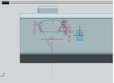
Fig. 4.6 2d sketch on dash board

Fig. 4.7 Dimple option of above 2d sketch

(7)

International Journal of Research

June 2019

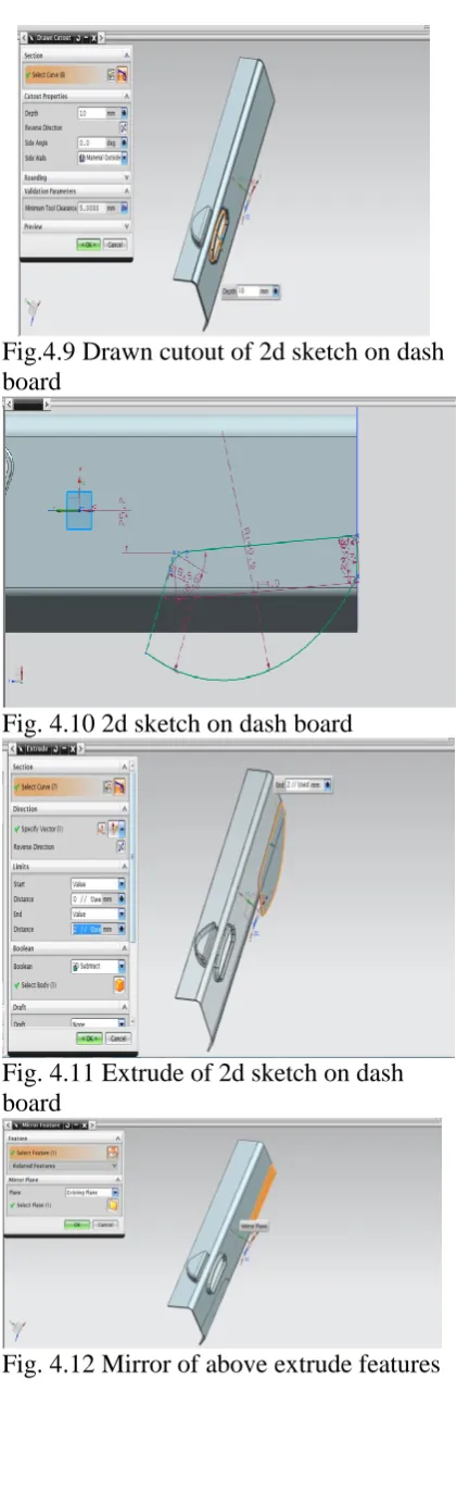
Fig.4.9 Drawn cutout of 2d sketch on dash board

Fig. 4.11 Extrude of 2d sketch on dash board

Fig. 4.12 Mirror of above extrude features

Fig. 4.14 Extrude of 2d sketch on dash board

Fig.4.15 Final 3D model of car dash board

4.2 MODIFIED DASH BOARD WITH 5.5 MM THICK

(8)

International Journal of Research

June 2019

Fig.4.17 Final 3D model of modified car dash board

MODAL ANALYSIS OF CAR DASH BOARD

5.1 INTRODUCTION ABOUT FEM

The Basic concept in FEA is that the body or structure may be divided into smaller elements of finite dimensions called “Finite Elements”. The original body or the structure is then considered as an assemblage of these elements connected at a finite number of joints called “Nodes” or “Nodal Points”. Simple functions are chosen to approximate the displacements over each finite element. Such assumed functions are called “shape functions”. This will represent the displacement within the element in terms of the displacement at the nodes of the element.

The Finite Element Method is a mathematical tool for solving ordinary and partial differential equations. Because it is a numerical tool, it has the ability to solve the complex problems that can be represented in differential equations form. The applications of FEM are limitless as regards the solution of practical design problems. Due to high cost of computing power of years gone by, FEA has a history of being used to solve complex and cost critical problems. Classical methods alone usually cannot provide adequate information to determine the safe working limits of a major civil engineering construction or an automobile or an aircraft.

In the recent years, FEA has been universally used to solve structural

engineering problems. The departments, which are heavily relied on this technology, are the automotive and aerospace industry. Due to the need to meet the extreme demands for faster, stronger, efficient and lightweight automobiles and aircraft, manufacturers have to rely on this technique to stay competitive.

FEA has been used routinely in high volume production and manufacturing industries for many years, as to get a product design wrong would be detrimental. For example, if a large manufacturer had to recall one model alone due to a hand brake design fault, they would end up having to replace up to few millions of hand brakes. This will cause a heavier loss to the company.

The finite element method is a very important tool for those involved in engineering design; it is now used routinely to solve problems in the following areas.

Structural analysis Thermal analysis

Vibrations and Dynamics Buckling analysis

Acoustics

Fluid flow simulations Crash simulations Mold flow simulations

Nowadays, even the most simple of products rely on the finite element method for design evaluation. This is because contemporary design problems usually cannot be solved as accurately & cheaply using any other method that is currently available. Physical testing was the norm in the years gone by, but now it is simply too expensive and time consuming also.

5.2 THE BASIC STEPS INVOLVED IN FEA

(9)

International Journal of Research

June 2019

element, the variation of displacement is assumed to be determined by simple polynomial shape functions and nodal displacements. Equations for the strains and stresses are developed in terms of the unknown nodal displacements. From this, the equations of equilibrium are assembled in a matrix form which can be easily be programmed and solved on a computer. After applying the appropriate boundary conditions, the nodal displacements are found by solving the matrix stiffness equation. Once the nodal displacements are known, element stresses and strains can be calculated.

Basic Steps in FEA are:

1. Descritization of the domain

2. Application of Boundary conditions 3. Assembling the system equations 4. Solution for system equations 5. Post processing the results.

Descritization of the domain: The task is to divide the continuum under study into a number of subdivisions called element. Based on the continuum it can be divided into line or area or volume elements.

Application of Boundary conditions:

From the physics of the problem we have to apply the field conditions i.e loads and constraints, which will help us in solving for the unknowns.

Assembling the system equations: This involves the formulation of respective characteristic (Stiffness in case of structural) equation of matrices and assembly.

Solution for system equations: Solving for the equations to know the unknowns. This is basically the system of matrices which are nothing but a set of simultaneous equations are solved.

Viewing the results: After the completion of the solution we have to review the required results.

The first two steps of the above said process is known as pre-processing stage, third and fourth is the processing stage and final step is known as post-processing stage.

5.3 STRUCTURAL ANALYSIS

Static analysis is one in which the loads/boundary conditions are not the functions of time and the assumption here is that the load is applied gradually. The most common application of FEA is the solution of stress related design problems.

Typically in a static analysis the kind of matrix solved is

[K] * [X] = [F]

Where K is called the stiffness matrix, X is the displacement vector and F is the load matrix. This is a force balance equation. Sometimes, the K matrix is the function X. Such systems are called non-linear systems.

Once the displacement vector {X} is known, the response quantities can be calculated.

5.4 INTRODUCTION TO ANSYS

ANSYS has evolved into multipurpose design analysis software program, recognized around the world for its many capabilities. Today the program is extremely powerful and easy to use. Each release hosts new and enhanced capabilities that make the program more flexible, more usable and faster. In this way ANSYS helps engineers meet the pressures and demands modern product development environment.

(10)

International Journal of Research

June 2019

across all platforms. ANSYS design data access enables user to import computer aided design models in to ANSYS, eliminating repeated work. This ensures enterprise wide, flexible engineering solution for all ANSYS user.

5.5 PROGRAM AVAILABILITY

The ANSYS program operates on 486 and Pentium based PCs running on Windows 95 or Window NT and workstations and super computers primarily running on UNIX operating system. ANSYS continually works with new hardware platforms and operating system.

Analysis types available:

1. Structural static analysis 2. Structural dynamic analysis 3. Structural buckling analysis

 Linear buckling  Non linear buckling 4. Structural non linearity

5. Static and dynamic kinematic analysis

6. Thermal analysis

5.6 PROCEDURE FOR ANSYS

Static analysis is used to determine the displacements, stresses, strains ad forces in structures or components due to loads that do not induce significant inertia and damping effects. Steady loading in response conditions are assumed. The kinds of loading that can be applied in a static analysis include externally applied forces and pressures, steady state internal forces such as gravity or rotational velocity imposed (non zero) displacements, temperatures (for thermal strain). A static analysis can be either linear or non-linear.

The procedure for structural analysis consists of these main steps:

1. Building the model 2. Obtaining the solution 3. Reviewing the results

Build the model:

In this step we specify the job name and analysis title, element types, real constants, material properties and geometry element types both linear and non-linear structural elements are allowed. The ANSYS element library contains over 80 different element types.

Material properties:

Young’s modulus (EX) must be defined for a structural analysis. If we need to apply inertia loads (such as gravity), we define mass properties such as density (DENS). Similarly, if we plan to apply thermal loads (temperatures), we define coefficient of thermal expansion (ALPX).

Obtain the solution:

In this step we define the analysis type and options, apply loads and initiate the finite element solution. This involves three phases

 Pre-processor phase  Solution phase  Post-processor phase

PRE-PROCESSOR:

Pre-processor has been developed so that the same program is available on micro, mini, super-mini and mainframe computer system. This slows easy transfer of models one system to other.

Pre-processor is an interactive model builder to prepare the FE model and input data. The solution phase utilizes the input data developed by the pre-processor, and prepares the solution according to the problem definition. It creates input files to the temperature etc., on the screen in the form of contours.

Model generation:

Two different methods are used to generate a model.

 Direct generation  Solid modelling

(11)

International Journal of Research

June 2019

shape of the elements and then instruct ANSYS program to generate all the nodes and elements automatically. By contrast, with the direct generation method, we determine the location of every node and size, shape and connectivity of every element prior to defining these entities in the ANSYS model. Although, some automatic data generation is possible (by using commands such as FILL, NGEN, EGEN etc). The direct generation method essentially a hands on numerical method that requires us to keep track of all the node numbers as we develop the finite element mesh. Solid modelling is usually more powerful and versatile than direct generation is commonly preferred method of generating a model.

Mesh generation:

In the finite element analysis the basic concept is to analyze the structure, which is an assemblage of discrete pieces called elements, which are connected together at a finite number of points called nodes. Loading boundary conditions are then applied to these elements and nodes. A network of these elements is known as mesh.

Finite element generation:

The maximum amount of time in a finite element analysis is spent on generating elements and nodal data. Pre-processor allows the user to generate nodes and elements automatically, at the same time allowing control over size and number of elements. There are various types of elements that can be mapped or generated on various geometric entities.

The elements developed by various automatic element generation capabilities of pre-processor can be checked element characteristics that may need to be verified before the finite element analysis for connectivity, distortion-index etc.

Generally, automatic mesh generating capabilities of pre-processor are used rather than defining the nodes individually. If required, nodes can be

defined easily by defining the allocations or by translating the existing nodes. Also one can plot, delete, or search nodes.

Boundary conditions and loading:

After completion of the finite element model it has to constrain and load has to be applied to the model. User can define constraints and loads in various ways.

Model display:

During the construction and verification stages of the model, it may be necessary to view it from different angles. It is useful to rotate the model with respect to the global system and view it from different angles. Pre-processor offers this capability. By windowing feature pre-processor allows the user to enlarge a specific area of the model for the clarity and details. Pre-processor also provides features like smoothness, scaling, regions, active set, etc for efficient model viewing and editing.

Material definitions:

All elements are defined by nodes, which have only their location defined. In the case of plate and shell elements there is no indication of thickness. The thickness can be given as element property. Different types of elements have different properties. For e.g.

 Beams: Cross sectional area, moment of inertia etc

 Shells: Thickness  Springs: Stiffness  Solids: None

The user also needs to define material properties of the elements. For linear static analysis, modulus of elasticity and Poisson’s ratio need to be provided. For heat transfer, coefficient of thermal expansion, densities etc are required.

SOLUTION:

(12)

International Journal of Research

June 2019

done by the computer and finally displacements are stress values are given as output. Some of the capabilities of the ANSYS are linear static analysis, non-linear static analysis, transient analysis etc.

POST-PROCESSOR:

It is powerful user-friendly post-processing program using interactive colour graphics. It has extensive plotting feature for displaying the results obtained from the finite element analysis. One picture of the analysis results (i.e. the results in a visual form) can often reveal in seconds, what would take an engineer hour to asses from a numerical output. The engineer may also see the important aspects of the results that could be easily missed in a stack of numerical data.

Employing state of art image enhancement techniques, facilities viewing of:

 Contours of stresses, displacements, temperatures etc.

 Deform geometric plots  Animated deformed shape  Time-history plots

 Solid sectioning  Hidden line plot

 Light source shaded plot  Boundary line plot etc.

The entire range of post processing options of different types of analysis can be accessed through the command/menu mode there by giving the user added flexibility and convenience.

5.7 MODAL ANALYSIS Methodology:

 Develop a 3D model.

 The 3D model is created using UNIGRAPHICS-NX software.

 The 3D model is converted into parasolid and imported into ANSYS to do modal analysis.

 Calculate natural frequencies and plot their mode shapes.

Natural Frequency:

Natural frequency is the frequency at which a system naturally vibrates once it has been set into motion. In other words, natural frequency is the number of times a system will oscillate (move back and forth) between its original position and its displaced position, if there is no outside interference.

The natural frequency is calculated from the formula given below. The natural frequencies depend on stiffness of the geometry and mass of the material.

Fundamental Natural Frequency

The fundamental frequency, often referred to simply as the fundamental, is defined as

the lowest frequency of

a periodic waveform. In terms of a superposition of sinusoids (e.g. Fourier series), the fundamental frequency is the lowest frequency sinusoidal in the sum.

Resonance:

In physics, resonance is the tendency of a system to oscillate with greater amplitude at some frequencies than at others. Frequencies at which the response amplitude is a relative maximum are known as the system's resonant frequencies, or resonance frequencies. At these frequencies, even small periodic driving forces can produce large amplitude oscillations, because the system stores vibration energy.

(13)

International Journal of Research

June 2019

systems have multiple, distinct, resonant frequencies.

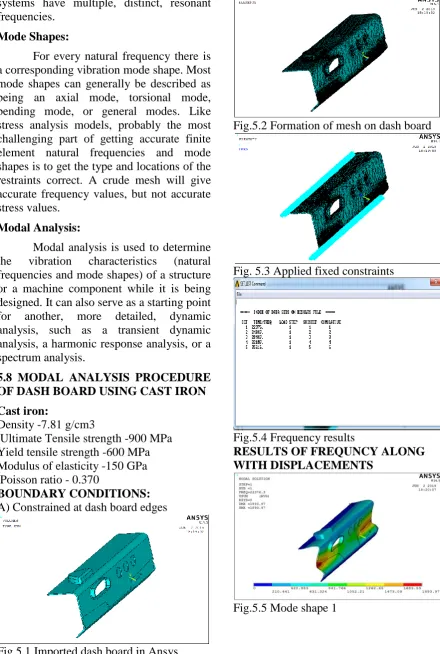
Mode Shapes:

For every natural frequency there is a corresponding vibration mode shape. Most mode shapes can generally be described as being an axial mode, torsional mode, bending mode, or general modes. Like stress analysis models, probably the most challenging part of getting accurate finite element natural frequencies and mode shapes is to get the type and locations of the restraints correct. A crude mesh will give accurate frequency values, but not accurate stress values.

Modal Analysis:

Modal analysis is used to determine the vibration characteristics (natural frequencies and mode shapes) of a structure or a machine component while it is being designed. It can also serve as a starting point for another, more detailed, dynamic analysis, such as a transient dynamic analysis, a harmonic response analysis, or a spectrum analysis.

5.8 MODAL ANALYSIS PROCEDURE OF DASH BOARD USING CAST IRON Cast iron:

Density -7.81 g/cm3

Ultimate Tensile strength -900 MPa Yield tensile strength -600 MPa Modulus of elasticity -150 GPa Poisson ratio - 0.370

BOUNDARY CONDITIONS:

A) Constrained at dash board edges

Fig.5.1 Imported dash board in Ansys

Fig.5.2 Formation of mesh on dash board

Fig. 5.3 Applied fixed constraints

Fig.5.4 Frequency results

RESULTS OF FREQUNCY ALONG WITH DISPLACEMENTS

(14)

International Journal of Research

June 2019

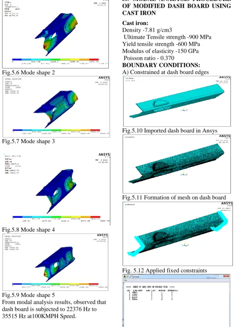
Fig.5.6 Mode shape 2

From modal analysis results, observed that dash board is subjected to 22376 Hz to 35515 Hz at100KMPH Speed.

5.9 MODAL ANALYSIS PROCEDURE OF MODIFIED DASH BOARD USING CAST IRON

Cast iron:

Density -7.81 g/cm3

Ultimate Tensile strength -900 MPa Yield tensile strength -600 MPa Modulus of elasticity -150 GPa Poisson ratio - 0.370

BOUNDARY CONDITIONS:

A) Constrained at dash board edges

Fig.5.10 Imported dash board in Ansys

Fig.5.11 Formation of mesh on dash board

(15)

International Journal of Research

June 2019

Fig.5.13 Frequency results

RESULTS OF FREQUNCY ALONG WITH DISPLACEMENTS

From modal analysis results, observed that dash board is subjected to 10022 Hz to 27514 Hz at100KMPH Speed. It formed less vibrations compared to previous. So it is a best for high speed.

MANUFACTURING OF MODIFIED CAR DASH BOARD

6.1 I INTRODUCTION OF CAM:

Computer-aided manufacturing (CAM) is the use of computer software to control machine tools and related machinery in the manufacturing of work pieces. This is not the only definition for CAM, but it is the most common; CAM may also refer to the use of a computer to assist in all operations of a manufacturing plant, including planning, management, transportation and storage. Its primary purpose is to create a faster production process and components and tooling with more precise dimensions and material consistency, which in some cases, uses only the required amount of raw material (thus minimizing waste), while simultaneously reducing energy consumption.

CAM is a subsequent computer-aided process after computer-aided design (CAD) and sometimes computer-aided engineering (CAE), as the model generated in CAD and verified in CAE can be input into CAM software, which then controls the machine tool.

(16)

International Journal of Research

June 2019

an effective CAD data exchange. Usually it had been necessary to force the CAD operator to export the data in one of the common data formats, such as IGES or STL, that are supported by a wide variety of software. The output from the CAM software is usually a simple text file of G-code, sometimes many thousands of commands long, that is then transferred to a machine tool using a direct numerical control (DNC) program.

CAM packages could not, and still cannot, reason as a machinist can. They could not optimize tool paths to the extent required of mass production. Users would select the type of tool, machining process and paths to be used. While an engineer may have a working knowledge of G-code programming, small optimization and wear issues compound over time. Mass-produced items that require machining are often initially created through casting or some other non-machine method. This enables hand-written, short, and highly optimized G-code that could not be produced in a CAM package.

Typical areas of concern:

 High Speed Machining, including streamlining of tool paths

 Multi-function Machining  5 Axis Machining

 Feature recognition and machining  Automation of Machining processes  Ease of Use

(17)

International Journal of Research

(18)

International Journal of Research

(19)

International Journal of Research

June 2019

RESULTS AND CONCLUSION

In this project is to develop the avoiding the noise in dashboard and generating G-codes and M-Codes for manufacturing process. Design of dashboard is done by NX-CAD and Modal analysis of dashboard is done by Ansys package. G-codes and M-Codes are generating by NX-CAM software.

From modal analysis results, observed that modified dash board is subjected to 10022 Hz to 27514 Hz at100KMPH Speed. It formed less vibrations compared to previous. So it is a best for high speed. Also NC program is generated.

REFERENCES

1. Akao Y (1994) Development history of quality function deployment. The customer driven approach to quality planning and deployment. Minato, Tokyo 107 Japan.

2. Akao Y (1990) Quality function deployment: A literature review. European Journal of Operational Research 143: 463-497.

3. Chan LK, Wu ML (2002) Quality function deployment: A literature review. European Journal of Operational Research 143: 463-497.

4. Cohen L (1995) Quality function deployment: How to make QFD work for you. (1stedn), Prentice Hall, New Jersey. 5. Dean EB (1998) Quality function deployment: From the perspective of competitive advantage. 6. Day RG

(1993) Quality function deployment: Linking a company with its customers. ASQC Quality press, Milwaukee.

7. Franceschini F (2002) Advanced quality function deployment. St. Lucie Press, Boca Raton, Fla.

8. Guinta LR, Praizler NC (1993) The QFD book: The team approach solving problems and satisfying customers through Quality function deployment. 9. Hunt RA, Killen CP (2004) Best practice

quality function deployment (QFD) cases. Emerald Group Pub, Bradford, England.

10. Hauser JR., Clausing D (1988) The house of quality. Harvard Business Review.

11. http://en.wikipedia.org/wiki/Computer-aided_design

12. Bossert JL (2000) Quality function deployment.

13. Martins A, Aspinwall EM (2001) Quality function deployment: an empirical study in the UK. Total Quality Management 12: 575-588.