Improving Neural Sequence Labelling Using Additional Linguistic Information

(1)

Scholarship@Western

Electronic Thesis and Dissertation Repository

4-23-2019 2:30 PM

Improving Neural Sequence Labelling Using Additional Linguistic

Information

Muhammad Rifayat Samee The University of Western Ontario

Supervisor Mercer, Robert E.

The University of Western Ontario Graduate Program in Computer Science

A thesis submitted in partial fulfillment of the requirements for the degree in Master of Science © Muhammad Rifayat Samee 2019

Follow this and additional works at: https://ir.lib.uwo.ca/etd

Part of the Artificial Intelligence and Robotics Commons

Recommended Citation Recommended Citation

Samee, Muhammad Rifayat, "Improving Neural Sequence Labelling Using Additional Linguistic Information" (2019). Electronic Thesis and Dissertation Repository. 6156.

https://ir.lib.uwo.ca/etd/6156

This Dissertation/Thesis is brought to you for free and open access by Scholarship@Western. It has been accepted for inclusion in Electronic Thesis and Dissertation Repository by an authorized administrator of

(2)

Acknowledgement

I would like to express my sincere gratitude to my thesis supervisor Dr. Robert E. Mercer.

Without his continuous guidance and significant contributions this work would not have been possible. Special thanks to my research colleague Mahtab Ahmed for his help and contributions

to this work.

I would like to thank the Department of Computer Science of The University of Western

Ontario for providing me with the Graduate Research Scholarship.

Last but not the least, I would like to thank my parents for believing in me and for providing

me with continuous support and encouragement throughout my graduate study.

(3)

Sequence Labelling is the task of mapping sequential data from one domain to another

domain. As we can interpret language as a sequence of words, sequence labelling is very

common in the field of Natural Language Processing (NLP). In NLP, some fundamental

se-quence labelling tasks are Parts-of-Speech Tagging, Named Entity Recognition, Chunking,

etc. Moreover, many NLP tasks can be modeled as sequence labelling or sequence to sequence

labelling such as machine translation, information retrieval and question answering. An exten-sive amount of research has already been performed on sequence labelling. Most of the current

high performing models are neural network models. These Deep Learning based models are

outperforming traditional machine learning techniques by using abstract high dimensional

fea-ture representations of the input data. In this thesis, we propose a new neural sequence model

which uses several additional types of linguistic information to improve the model

perfor-mance. The convergence rate of the proposed model is significantly less than similar models.

Moreover, our model obtains state of the art results on the benchmark datasets of POS, NER,

and chunking.

Keywords: Sequence Labelling, Neural Network, Deep Learning, NLP

(4)

List of Figures

1.1 Example of POS tagging . . . 2

1.2 Example of NER tagging . . . 3

1.3 Example of Chunking . . . 4

2.1 Recurrent Neural Network (RNN) [6] . . . 7

2.2 Long Short Term Memory Unit (LSTM) and Gated Recurrent Unit (GRU) . . . 9

2.3 Word2Vec Models [31] . . . 10

2.4 Convolutional Neural Network (CNN) for Character level representation [25] . 12 2.5 Long Short Term Memory Unit (LSTM) for Character level representation [22] 13 2.6 Word Sequence Representation [56] . . . 14

3.1 Character Embedding for the Word cats . . . 20

3.2 Pick Up Character Embedding . . . 21

3.3 CW, R, CO connection . . . 26

3.4 BLSTM-CRF model architecture . . . 27

(7)

2.1 Performance on CoNLL 2003 (NER) . . . 18

2.2 Performance on CoNLL 2000 (Chunking) . . . 18

2.3 Performance on WSJ (POS tagging) . . . 18

4.1 Dataset Description . . . 29

4.2 Ranges of different hyper-parameters. . . 30

4.3 Comparison of F1 scores of different models for chunking . . . 31

4.4 Comparison of F1 scores of different models for NER . . . 31

4.5 Comparison of Accuracy of different models for POS tagging . . . 32

4.6 Training time (hours) of our BLSTM-CRF model on the WSJ corpus compared with all models of [24] using the same hardware configuration (GPU: Nvidia GTX 1080) . . . 32

4.7 Change inwi’s for each module with epochs. . . 33

4.8 Ablation study of our BLSTM-CRF model for POS tagging. (R - Residual connection, CW - Concatenate with word embedding, CO - Concatenate with second last output layer) . . . 34

(8)

Chapter 1 Introduction

In Natural Language Processing, often we need to find a function to map sequence pairs from

different domains. An example of such sequence pairs is a sequence of words(i.e, a sentence)

and a sequence of parts-of-speech. This is the well-known parts-of-speech (POS) tagging

problem. Formally, given an input sequenceX = x1,x2, ...,xn where eachxi is from a domain

αand a corresponding tagging/state sequenceY =y1,y2, ...,ynwhere eachyi is from a domain

γ, our goal is to find a functional mapping f : X 7→ Y. For example, in the POS tagging

problem one possible input sequence might be"France won the Match". The corresponding

POS tagged sequence will be N V D N. Here N, V, and D represent tags for Noun, Verb,and

Determiner,respectively. In this example, our function f maps word sequences to their possible parts-of-speech sequences.

Sequence Labelling can be treated as a supervised machine learning task. Givenmtraining

examples (x(i),_y(i)_{) for}_i = _{1 . . .}_m_{where each} _x(i) _{is a sentence}_x(i) 1 . . .x

(i)

ni of lengthni, and each

y(i) _{is a tag sequence}_y(i) 1 . . .y

(i)

ni of lengthni, our task is to train a model to correctly predict the

tagged sequenceYfor an unknown input sentenceX. In this chapter we briefly introduce some

fundamental sequence labelling problems. Moreover, we give an introduction to our approach

and will give the outline of this thesis.

1.1 Some Sequence Labelling Problems in NLP

1.1.1 Parts-of-Speech (POS) Tagging

Parts-of-speech (POS) Tagging is probably the oldest and most famous sequence labelling

problem in the field of Natural Language Processing. In this problem the goal is to map each

word of a sentence to its correct POS. Extensive research has been performed on POS tagging.

Among all the sequence labelling problems, POS tagging is treated as an almost solved

(9)

lem with state of the art accuracy being between 97% and 98% [24]. In 2011, C. Manning [26]

argued that, to go from 97% to 100%, we need to explore more linguistic features. His idea is

reflected in the recent deep learning architectures where along with features which are

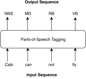
implic-itly extracted by Neural Networks, researchers are incorporating carefully designed linguistic features. Figure 1.1 shows an example of POS tagging. The input sequence is "cats can not

fly" and the corresponding POS tags are NNS (plural common noun), MD (modal auxiliary),

RB (adverb) and VB (verb).

Parts-of-Speech Tagging

Cats

can

not

Input Sequence

Output Sequence

ﬂy

NNS

MD

RB

VB

Figure 1.1: Example of POS tagging

1.1.2 Named Entity Recognition (NER)

Named Entity Recognition is another sequence labelling problem: the input sequence is a

sentence and the output sequence is the sentence tagged with possible named entities. Some

common named entities are persons, organizations, locations and names. Named entity recog-nition is challenging because a large amount of feature and lexicon knowledge is required to

achieve high performance. Most of the high performing models for the NER task are

neu-ral network models. Current state of the art F1 score (4.1.3) for English NER task is around

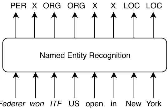
91%. Figure 1.2 shows a simple example of NER task. The input sentence is "Federer won

ITF US open in New York". And the NER model identifies Federer as a "PERSON", ITF as

(10)

1.2. OurApproach 3

Named Entity Recognition

Federer won ITF

Input Sequence Output Sequence

US open in New York

PER X ORG ORG X X LOC LOC

Figure 1.2: Example of NER tagging

1.1.3 Chunking ( Shallow Parsing)

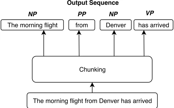
Chunking, also known as shallow parsing, is the task of dividing texts to syntactically

corre-lated sequence of words. For example: "The morning flight from Denver has arrived." can

be divided as"[NP The morning flight ] [PP from] [NP Denver] [VP has arrived]". Here the

syntactic constructs are noun phrase (NP), verb phrase (VP) and preposition (PP). This shallow parsing can be an intermediate step before parsing a sentence. Chunking can be designed as a

sequence labelling task where each word of the same chunk will be tagged with the same label.

Unlike POS tagging and NER, for Chunking, most of high performing models are not neural

models. The Best F1-score of 95.23% is achieved by Shen et al. [46] using a Hidden Markov

Model with a voting scheme.

1.2 Our Approach

In this thesis, our goal is to improve neural sequence labelling by using additional linguistic

features. We propose a new neural architecture for the Sequence Labelling problem which is

capable of using several linguistic features to improve tagging accuracy. In our approach we

used sense embedding along with word level knowledge to capture semantic features.

More-over, to capture morphological features we used character level embeddings for words.

(11)

Chunking

The morning ﬂight from Denver has arrived The morning ﬂight

NP

from Denver

NP PP

has arrived

VP

Input Sequence Output Sequence

Figure 1.3: Example of Chunking

(LSTM)[16] to capture contextual and morphological features simultaneously. We used a

Con-volutional Neural Network (CNN) to exploit bigram(two adjacent words) information. Several

hand crafted spelling features (prefix, suffix, patterns) were used with the implicit neural fea-ture extraction done by the Deep Neural Learning. To connect all the feafea-tures appropriately we used three connection methods: Residual connection, Concatenate with word embedding and

Concatenate with second last output layer. Our architecture achieved state of the art results on

benchmark datasets of POS tagging, NER and Chunking without using any additional data or

multi-task learning.

1.3 Thesis Outline

This thesis is organized in four chapters. In the second chapter we summarize previous work done in sequence labelling using Deep Neural Networks. We discuss the main components of

a typical deep sequence labelling model. Chapter 3 details our proposed model. For each of

the modules of our model, we talk about the reason behind using the module and the detail

functionality of the module. Chapter 4 is dedicated to experimental results. In this chapter, we

show our experimental setup and discuss our experimental findings. We compare our results

with several state of the art models on different benchmark data sets for POS, NER and the

Chunking task. Moreover, we do an ablation study of our model to see the impact and

useful-ness of different modules of our architecture. We also discuss feature connection methods used

(12)

Chapter 2 Related Work

In this chapter we summarize previous work done on the sequence labelling task. First we

give an overview of the previous work for Parts-of-speech (POS) tagging using traditional

ap-proaches. Then we present a summary of research work using Deep Neural Architectures for

sequence labelling tasks. Then we introduce some well-known and commonly used

architec-tures and techniques for Deep Sequence Labelling Networks. Finally, we compare several Deep learning based models on benchmark datasets for the sequence labelling task.

2.1 Previous Work

2.1.1 Statistical Sequence Labelling Models

Before the advancement of Deep Learning, most of the high performing models for sequence

labelling were Statistical in nature. Models were based on Hidden Markov Models (HMMs)

[12, 59] and Conditional Random Fields (CRFs) [21, 33]. For example, Weischedel et al. [55]

introduced a generic n-gram probabilistic model for sequence labelling. They experimented

using tri-gram version of their model on the WSJ corpus for POS tagging, achieving 96.3%

accuracy. Their experimental result showed that probabilistic models are capable of extracting

lexical features which can replace rule based systems. Even though this paper used several

features to deal with the sparsity problem, the paper did not talk about clear ways to incorpo-rate features to make the model’s feature space more robust. The Maximum-Entropy Model

[40] introduced a way to incorporate an arbitrary number of binary features into the

proba-bilistic model. As expected, the Maximum-Entropy model achieved better accuracy than the

tri-gram model on unknown words (85.6%) which leads to overall accuracy of 96.6%. The

next improvement on overall accuracy came from a Hidden Markov model using second-order

approximations. The model proposed by Scott and Harper [52] uses a 3d transition probability

(13)

matrix which not only depends on the current state but also on the previous state. Moreover,

they used a separate parameter for unknown words. The model got 96.9% accuracy on the WSJ

corpus, which is an improvement over the previous models. However, the unknown word

ac-curacy (84.9%) is significantly less than the Maximum-Entropy model. The reason behind it is

that the Second-Order Markov model did not use any hand-crafted features. It only uses

statis-tical approximations from the data. The experimental results of the three statisstatis-tical approaches

described above clearly indicate that, for supervised sequence labelling problems using only

probabilistic parameter estimation is not enough. We need to exploit specialized features to

boost model accuracy.

2.1.2 Deep Learning models for Sequence Labelling

In the past few years, Deep Neural Network architectures became very popular in the field

of Natural Language Processing (NLP). Recent advancements in distributional word

repre-sentation and Recurrent Neural Networks (RNN) made neural architectures superior to the

traditional statistical machine learning techniques in almost every NLP tasks. All of the

archi-tectires and other techniques used in this and the next paragraph will be decribed in the next

sections.

Huang et al. [17] propose a few models for the sequence tagging task. Apart from just word

embeddings, they use morphological, bigram and trigram information as their input features.

Later, they use Long Short Term Memory (LSTM) and Bidirectional LSTM (BLSTM) with Conditional Random Field (CRF) to do the final tagging. Lample et al. [22] extract character

embeddings from both the left and right directions, concatenate these with word embeddings

and use a stacked LSTM with CRF to do the tagging. Liu et al. [24] propose a model leveraging

word and character level features. It includes a language model to represent the character level

knowledge along with a highway layer to avoid the feature collision. Finally it is trained jointly

as a multitask learning. Yu et al. [57] propose a general purpose tagger using a Convolutional

Neural Network (CNN). First, they use CNNs to extract the character level features and then

concatenate it with word embeddings, position embeddings and binary features. Finally they

use another CNN to get the contextual features as well to do the tagging. Ma and Hovy [25] propose an end-to-end sequence labelling model using a combination of BLSTM, CNN and

CRF. They use a CNN to get the character level information, concatenate it with word

embed-dings and then apply BLSTM to model the contextual information. Finally they generate the

tags by using a sequential CRF layer. Rei [41] trains a language model type objective function

using BLSTM-CRF to predict the surrounding words for every word in the corpus and utilizes

(14)

2.2. RecurrentNeuralNetwork(RNN) 7

In the next portion of this chapter, we will study commonly used architectures and

tech-niques for a typical Deep Neural Sequence Labelling model. At the end of the chapter, we will

compare different neural models on three sequence labelling tasks: POS tagging, NER and

Chunking on benchmark datasets.

2.2 Recurrent Neural Network (RNN)

Traditional feedforward neural networks cannot capture dependencies in sequential data. For

this reason, feedforward neural networks are not suitable for natural language where past

con-text is important to predict the future. For example: let’s consider predicting the word “

de-feated” in the sentence"France won the World cup final 2018, so they defeated Croatia 2-1 in the final". To predict “defeated” we need to remember the inputs from earlier in the sentence. Being a bipartite graph, a feedforward neural network does not have the mechanism to address

this issue. Recurrent Neural Networks (RNN) are specially designed to have internal memory

to remember some important portion of the previous data to predict the future events. RNNs

have loops that allow information to persist. Figure 2.1 shows a typical RNN structure. There,

xt is the input at time step tand the ot is the corresponding output at time step t. W,V ,U are

the parameters of an RNN. All the parameters are shared across time steps. So the outputot+1

is influenced by all the previous inputsxt,xt−1. . .x1and the current input data xt+1.

Figure 2.1: Recurrent Neural Network (RNN) [6]

Long Short Term Memory Unit (LSTM)

Theoretically, Recurrent Neural Networks are supposed to capture long distance dependencies

(15)

of the gradient vanishing/exploding problem [5] [35]. Long Short Time Memory Units (LSTM) are designed to capture long distance dependencies without succumbing to the gradient

van-ishing/exploding problem. LSTMs were first proposed by Hochreiter and Schmidhuber [16]

in 1997. LSTMs have three multiplicative gates: input gate, forget gate and output gate. Each gate has a transformation matrixWi,Wf andWorespectively. All the gates are sigmoid gates so

the output of the gates are between 0 and 1. Using the gates, an LSTM decides what

informa-tion from the past time step should be remembered. Fig 2.2(a) shows the internal structure of

an LSTM cell.Ct−1andht−1are the cell state and hidden state at time stept−1. First the forget

gate decides what portion of theCt−1 we want to forget (eq 2.1) by using a sigmoid activation

on the linearly transformed representation of the concatenation of the previous hidden stateht−1 and the current input vector xt. In the equation, [ht−1,xt] means the concatenation operation of

two vectors: ht−1 and xt. Then the input gate decides which new values we need to update by

seeing the previous hidden state ht−1 and the current input xt (eq 2.2). A candidate cell state

¯

Ct is calculated by a tanh() layer (eq 2.3) (here ∗ is the point-wise multiplication function).

Finally the new cell state is created using the outputs from the forget gate and the input gate

(eq 2.4). Now to find the new hidden representation for the current time stept, LSTM uses the

new cell stateCtand the output of the output gateot (eq2.5) (eq2.6).

ft =σ(Wf.[ht−1,xt]+bf) (2.1)

it =σ(Wi.[ht−1,xt]+bi) (2.2)

¯

Ct = tanh(Wc.[ht−1,xt]+bc) (2.3)

Ct = ft∗Ct−1+it∗C¯t (2.4)

ot =σ(Wo.[ht−1,xt]+bo) (2.5)

(16)

2.3. DistributionalRepresentation ofWords 9

Figure 2.2: Long Short Term Memory Unit (LSTM) and Gated Recurrent Unit (GRU) [34]

Gated Recurrent Units (GRU)

A widely used and very popular variation of LSTM is Gated Recurrent Units (GRU). GRU was

proposed by Cho, et al. [9] in 2014. In GRUs the forget gate and input gate are combined into

a single update gate. So, GRUs have fewer parameters compared to LSTMs. For this reason,

unlike LSTMs, GRUs are less prone to over-fitting. Fig 2.2 (b) shows the structure of a single

GRU unit. Another major difference between LSTMs and GRUs is that the GRU structure does

not include any cell state. Updating the hidden state of a GRU unit is done as following:

zt = σ(Wz.[ht−1,xt]) (2.7)

rt = σ(Wr.[ht−1,xt]) (2.8)

¯

ht =tanh(W.[rt∗ht−1,xt]) (2.9)

ht =(1−zt)∗ht−1+zt ∗h¯t (2.10)

2.3 Distributional Representation of Words

Representing words as continuous vectors in a vector space (word embeddings) has been

ex-tensively researched. Bengio et al. [4] first proposed a neural architecture to find vector

repre-sentation of words. This model is mainly designed for estimating a neural network language

model (NNLM). The model is a feedfoward neural network with a linear projection layer and

a non-linear hidden layer. This idea of learning word representations using a neural network

(17)

2.3.1 Word2Vec

In 2013, Mikolov et al. [31] proposed a method to estimate high quality word vectors from huge

datasets. They proposed two different models: Continuous Bag of Words Model (CBOW)

and Continuous Skip-Gram model. Both models use a shallow neural network with one

hidden layer. These models use a fixed length context window for each target word. In

CBOW, the model predicts the target word from the context words. CBOW is similar to

the feedforward NNLM model where the projection layer is shared for all the words. On

the other hand, the Skip-Gram model predicts the context words from the target word.

Fig-ure 2.3 shows the model architectFig-ures. The result of the Skip-Gram model is very

surpris-ing. When the model is trained on a huge amount of data, the resulting vectors can capture

subtle semantic relationships between words. Moreover, it is possible to do meaningful

al-gebraic operations on the word vectors. For example: the resulting vector of the expression:

vector(“biggest00)−vector(“big00)+vector(“small00) is very close to the vector(“smallest00). Here, distance is measured by the cosine similarity of the vectors. Using pretrained word2vec

vectors, most of the neural NLP models get significant improvements in performance.

Nowa-days, it is common practice to use word vectors trained on extremely large amount of data for

initializing embedding layers of neural models.

(18)

2.4. CharacterLevelRepresentation inNeuralNetwork 11

2.3.2 GloVe: Global Vectors for Word Representation

Two main ideas for learning word vectors are the global matrix factorization method, such as latent semantic analysis (LSA) [11] and the fixed local context window method, such as the

Skip-Gram model [31]. The limitation of LSA and other global matrix factorization methods

is that the similarity measures of the vectors are dominated by the frequent words. On the

other hand, the Word2Vec Skip-gram model concentrate only on local context information and

fails to leverage global statistical information. In 2014 Pennington et al. [37] proposed a new

regression model which combines the advantages of the global matrix factorization method

and the local context features. Global Vectors (GloVe) first builds a co-occurrence matrixXof

a fixed window size. Xi j represents the number of times word jappears in the context of word

i. Then, GloVe tries to predict the co-occurrence ratio from the word vectors. For example, if

w∈Rd_{are word vectors and ¯}

w∈Rd _{are separate context word vectors then the basic equation is}

the following:

F(wi,wj,w¯k)≈

Pik

Pjk

(2.11)

Here Pik

Pjk is the ratio of co-occurrence probabilities. As one of the goals of GloVe is to find a

linear relation between the word vectors, it is possible to restrict the equation to the difference between the word vectors:

F(wi−wj,w¯k)≈

Pik

Pjk

(2.12)

The final loss function used by GloVe is the following:

J =

V

X

i,j=1

f(Xi j)(wTi wj+bi+b¯j−log(Xi j))2 (2.13)

(here V is the vocabulary size. The full mathematical simplification and optimization is not

included here.)

GloVe vectors outperform Word2Vec vectors in several NLP tasks including word analogy,

word similarity and Name Entity Recognition task. There is no significant different between

Word2Vec and GloVe in terms of performance, but with GloVe vectors it is easy to parallelize

the model. Thus GloVe can be trained a lot faster than Word2Vec.

2.4 Character Level Representation in Neural Network

In Neural Network architectures, words are represented using word embeddings. The Word

(19)

Word2Vec or Glove. To capture character level features, neural network models often

con-catenate character representations of words with their corresponding word embeddings. Other

research [10][17][49] has used feature look up tables to represent several character level

fea-tures like prefix, suffix, capitalization, etc. However, they have used predefined character level features. To extract features implicitly, a separate Neural Network model can be used.

2.4.1 Convolutional Neural Network for Character Level Representation

Convolutional Neural Networks (CNN) were first introduced by [43] for character embeddings.

They used a convolution kernel to produce local features for each character of a word and then used a max-pooling operation to produce a fixed length character embedding for that word.

Later, this idea of using CNN for character representation was used by [8][25][44]. Figure 2.4

shows the network used by [25] on the wordPlaying. First they used a convolution kernel of

size 3 over the padded character sequence of the word. Then the model used max-pooling to

create a vector representation of size 4 for the word Playing. In addition to that, a drop-out

layer[48] was used after the max-pooling layer.

(20)

2.5. WordSequenceRepresentation inNeuralNetwork 13

2.4.2 Long Short Term Memory Units for Character Level

Representa-tion

Bi-directional Long Short Term Memory Units (Bi-LSTMs) can also be used for finding

char-acter embeddings for words [22]. Figure 2.5 shows the Bi-LSTM model used by [22]. The

model uses two layers of LSTM named forward LSTM and backward LSTM. Forward LSTM captures features by going over the character sequence from left to right. The backward LSTM

captures features in the right to left direction. Then a single character representation vector is

created by concatenating the forward LSTM output and the backward LSTM output.

Figure 2.5: Long Short Term Memory Unit (LSTM) for Character level representation [22]

2.5 Word Sequence Representation in Neural Network

After extracting a feature vector for each word of a sentence from its corresponding character

sequence, each word is represented with a vector which is the result of a simple concatenation

of the word embedding vector and the character level feature vector for that word. Now using

(21)

Figure 2.6: Word Sequence Representation [56]

Like character representation, CNN and LSTM can be used to model word sequence

informa-tion. LSTM is the more popular choice for word sequence representation because we can

ex-tract features from both forward and backward direction of a sentence.[8][17][22][25][38][43]

used LSTM for word sequence representation. [10] used CNN for word sequence

representa-tion. Figure 2.6 (a) and (b) shows the Word CNN and Word LSTM architecture respectively.

The figure shows the way to represent the sentence"COLING is held in New Mexico". As the

figure indicates, the idea is similar to character level representation. The Word CNN model

uses multiple layers of convolution over the word vector representation of the sentence and

finally uses a linear layer to map the representation to the inference layer. Word LSTM model

uses one or more layers of Bi-LSTM over the word vectors to capture forward and backward

representation of the sentence. Finally the sentence vector for each time step is calculated by

concatenating the forward and backward vector of that time step. The final layer (the inference

layer) in both architectures uses either Softmax or CRF. These inference layers are discussed

in the next section.

2.6 Inference Layer in Neural Network

In sequence labelling models, after finding the word sequence representation of the sentence,

we need to assign desired labels to the word sequence. The Inference layer takes the word

sequence level representation as input and assigns labels to the word sequence. Softmax and

Conditional Random Field (CRF) are two commonly used inference layers for Neural

(22)

2.7. UsingHandCraftedFeatures inNeuralNetworks 15

2.6.1 Softmax Inference

Softmax is a normalized exponential function. The function can be written as:

σ(xi)=

exi

P

jexj

Herexiis theith component of the vectorx. We can first map the word sequence representation

to the label vocabulary by using a linear fully connected layer. After that, the softmax function can be applied on the mapping to generate a probability distribution over the label

vocabu-lary. However, softmax does not generate conditional probabilities so dependencies between

neighbouring labels cannot be considered. So for tasks with strong output label dependencies

Conditional Random Fields (CRF) is a better choice than the Softmax inference.

2.6.2 Conditional Random Fields (CRF)

In sequence Labelling problems it is often better to consider correlations between neighbour-ing labels to find the best possible taggneighbour-ing sequence. For example, for the POS task, it is

more likely that an adjective is followed by a noun rather than a verb. To capture this kind of

label dependency while finding the most probable tagging sequence, we can use Conditional

Random Fields (CRF). CRF is a Markov network over the labels, which specifies a conditional

probability distribution. Given an input sequenceZ ={z1,z2, ...,zn}and the corresponding label

sequenceY = {y1,y2, ...,yn}, CRF defines a family of conditional probabilities over all possible

label sequences y given z as follows:

p(y|z;W,b)=

Qn

i=1χi(yi−1,yi,z)

P

¯

y∈γ(z)

Qn

i=1χi( ¯yi−1,y¯i,z)

whereW,bare the parameters of the model andχi( ¯yi−1,y¯i,z)= eW

T ¯

y,yzi+b¯y,y _{is the potential}

func-tion. We will describe χi further in Section 3.6. CRFs are trained by maximizing conditional

likelihood of p(y|z;W,b). And the Viterbi algorithm [39] is used to find the label sequencey∗ with the highest conditional probabilityy∗ =argmaxy∈γ(z)(y|z;W,b).

2.7 Using Hand Crafted Features in Neural Networks

One of the main advantages of using Deep Neural Networks is that neural models can find

(23)

fea-tures along with the implicit feafea-tures found by the Neural Networks can improve the overall

performance. Most of the best performing models [10],[17],[49] use handcrafted features in

their model. Two kinds of handcrafted features were used by [17]: spelling features and

con-textual features. There was a total of 12 spelling features for a given word. Some examples

of spelling features are: whether the word starts with capital letter, whether the word only

consist of capital letters and is the word made with letter and digits. As contextual feature

they usedUni-gram,Bi-gram and Tri-Graminformation. There are different ways to introduce

handcrafted features in a neural model. Handcrafted features can be treated as word features

and can be concatenated with the word vectors. Another way is to connect the features directly

to the output layer just before doing the inference. The experimental results of [17] showed that

handcrafted features as word features have the same tagging accuracy as the direct connection.

However, direct connection is much faster and accelerated training of the model significantly.

2.8 Performance Comparison Between Neural Network

Mod-els

In the previous sections, we introduced the main components of a neural architecture for

se-quence labelling. Now we compare different models for three sequence labelling problems:

POS tagging, NER and Chunking. Comparing Neural Networks is difficult. Neural Networks

are very sensitive to hyperparameters. Moreover, datasets used are different from model to

model. Models use different training-development-test splits of the same dataset. For example,

different development sets for Chunking were used by [24] and [15]. Also for different models

the ways to use the development set are different. For instance, the development set has been

used only for hyper parameter tuning in [22][25] while the development set has been included

into the training in [8][38]. We try to compare the models as fairly as possible. For each of the

sequence labelling tasks we present a performance table on a specific benchmark dataset. All

tables have 6 columns:

• Model: Name of the model.

• Word Seq: Technique used for word sequence representation.

• Char Seq: Technique used for Character representation.

• Inference: Inference layer used.

(24)

2.8. PerformanceComparisonBetweenNeuralNetworkModels 17

• F1-score/Accuracy: Performance metric for the task.

Table 2.1 shows the performance of several models on the CoNLL 2003 dataset [54] for the

NER task. The best performing model uses LSTM to find the word sequence representation, CNN for character embeddings and CRF for inference [25]. However the model does not

use any handcrafted features. Table 2.2 shows performance comparison for the chunking task

on CoNLL 2000 dataset [53]. For chunking, the best F1-score of 95.00% with LSTM for

word sequence representation, CNN for character representation and CRF inference layer [38].

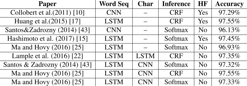
Table 2.3 shows the performance comparison among several models on POS tagging task.

The data set used for the comparison is the WSJ corpus [28]. For POS tagging two different

models get the same best accuracy of 97.55% [17][25]. Both of the models use LSTM for word

sequence and CRF for inference. CNN for character embedding was used by [25]. However,

instead of using any character level LSTM/CNN, handcrafted features to capture character

level features was used by [17]. Careful analysis of the performance tables yield insights about

neural sequence labelling models.

• For all the three tasks, models with character representation performed much better than

models which do not use any character LSTM/CNN.

• Observing POS tagging, two models attain the best performance [17][25], handcrafted

character features are used by only one of the methods [17]. This is a possible indication

that, if we can avoid possible feature collision, we can use character embedding and

handcrafted features together to boost model performance.

• For all three tasks, word-LSTM is better than word-CNN. Sometimes significantly [10][25].

• Char-CNN is superior to Char-LSTM for all the three tasks. However, in some cases the

performance difference of Char-LSTM and Char-CNN might not be significant for POS

tagging [22] and [25].

• As expected, CRF is better than Softmax for NER task. We expect CRF to be better

because CRF considers dependencies between labels and the NER task has strong label

(25)

Model Word Seq Char Inference HF F1-score

Collobert et al.(2011) [10] CNN – CRF Yes 89.59%

Huang et al.(2015) [17] LSTM – CRF Yes 90.10%

Lample et al. (2016) [22] LSTM – CRF No 90.20%

Strubell et al. (2017) [49] LSTM – CRF Yes 90.43%

Strubell et al. (2017) [49] LSTM – Softmax Yes 89.34%

Ma and Hovy (2016) [25] LSTM – Softmax No 87.00%

Chiu & Nichols (2016) [8] LSTM CNN CRF No 90.91%

Peters et al. (2017) [38] LSTM CNN CRF No 90.87%

Ma and Hovy (2016) [25] LSTM CNN CRF No 91.21%

Lample et al. (2016) [22] LSTM LSTM CRF No 90.94%

Table 2.1: Performance on CoNLL 2003 (NER)

Paper Word Seq Char Inference HF F1-score

Zhai et al. (2017) [58] LSTM – Softmax No 94.13%

Hashimoto et al. (2017) [15] LSTM – Softmax Yes 95.02%

Rei (2017) [42] CNN LSTM CRF No 93.15%

Peters et al. (2017) [38] LSTM CNN CRF No 95.00%

Table 2.2: Performance on CoNLL 2000 (Chunking)

Paper Word Seq Char Inference HF Accuracy

Santos&Zadrozny (2014) [43] CNN – Softmax No 96.13%

Hashimoto et al. (2017) [15] LSTM – Softmax Yes 97.45%

Ma and Hovy (2016) [25] LSTM – Softmax No 96.93%

Lample et al. (2016) [22] LSTM LSTM CRF No 97.35%

Santos & Zadrozny (2014) [43] LSTM CNN Softmax No 97.32%

Ma and Hovy (2016) [25] LSTM CNN CRF No 97.55%

Ma and Hovy (2016) [25] LSTM CNN Softmax No 97.33%

(26)

Chapter 3 Proposed Model

In this chapter we will talk about our proposed model for Sequence Labelling tasks. The

main contribution of the proposed model is it integrates word sense embeddings with word

level features — word embeddings, and morphological features — character embeddings. And

then our model uses novel ways to connect these embeddings with the ouput of a Convolutional

Neural Network (CNN), a Bidirectional Long Short Term Memory (BLSTM) and a Conditional

Random Field (CRF) module. We will describe each of the modules in detail. We will also

explain all the morphological and semantic features that we have used to improve our model.

Figure 3.4 in Section 3.8 shows our proposed model structure which is a reference for all the

module that we are going to describe in detail.

3.1 Word Embedding Module

For any neural network learning, we need to project the lexicons in some vector space. The

main motivation of using higher dimensional word vectors is to capture word level features.

One obvious way of extracting word level features is to randomly initialize the embeddings

and tune them with gradient optimization. However, we can also initialize the vectors with

pretrained word vectors like Word2Vec and Glove 2.3 and tune them with the model during

training phase. Pre-trained vectors are trained with huge datasets and these vectors are capable

of capturing semantic and syntactical relationships between the words. For this reason most of the time, using pre-trained vectors for initialization of the word vectors gives better results

than relaying on random vectors. We initialized our word embedding module with random

embeddings and pretrained embeddings (Glove/Word2Vec). We represent each sentence as a

column vector Imx1 where each element in the vector is a unique index of the corresponding

word. Here m is the length of the sentence. The word embeddings module transforms the

column vector Imx1 into a matrixWmxd. Each of the row of the matrix isddimensional which

(27)

represent the corresponding word vector.

3.2 Character Embedding Module

Character Embedding Module is used to capture morphological features of each word. For

example, for the wordhourly, the suffix-lygives us a good indication that,hourlyis an adverb.

To learn this kind of low level morphological features, we first represent a word as a Ck×1

column matrix wherekis the number of characters for that word. Then we used a embedding

layer to initialize random embeddings of dimentionn for each of the characters. So now the

word is represented by a matrixCk×n. After that, we run an LSTM on the matrix and used the

last hidden stateC1×n as the character embedding of the word. So if a sentence hasmwords

then the character level representation of the sentence will be a matrixCm×n where each row

C1×n is the character embedding of the corresponding word found by the LSTM. Figure 3.1

shows how the embedding for the word "cats" is calculated using 4 unfoldings of an LSTM

cell.

L S T M

Character Embeddings

c a t s

Figure 3.1: Character Embedding for the Word cats

3.3 Selective Pickup from Char-LSTM

Word embeddings are used to capture contextual features. On the other hand Character

Embed-ding Module described in Section 3.2 can extract morphological features of a word. To capture

both morphological and contextual features of a sentence together, we introduce a new way of

using a BLSTM network. First each sentence is represented in character level by a vectorIk×m

wherek is the number of characters in the sentence and m is the total words. Then we used

an embedding layer to represent each of thekcharacters inddimensional vectors. So now we

have a matrix of sizek×m×d. Now we run a BLSTM over the character sequence representing

the whole sentence. While running the BLSTM we picked up the hidden state from the time

(28)

3.4. WordSenseEmbeddings usingAdaptiveSkip-Gram 21

words as well as character sequence up to that time step in both direction.

˜

Cm×d = SELECT(BLSTM(I(k×m)×d)) (3.1)

Figure 3.2 shows the Selective Pickup module in action for the sentence"cats can not fly".

L S T M L S T M L S T M L S T M L S T M L S T M L S T M L S T M L S T M L S T M L S T M L S T M L S T M

C a t s c a n n o t f l y 1st Pick Up 2nd Pick Up 3rd Pick Up

Last Pick Up Last Pick Up

Figure 3.2: Pick Up Character Embedding

3.4 Word Sense Embeddings using Adaptive Skip-Gram

Knowing the sense of a word prior to tagging makes the tagging task more straightforward.

Generally, polysemy is captured in standard word vectors, but the senses are not represented as

multiple vectors. So we have trained an adaptive skip gram model, AdaGram, [3] which gives

a vector for each sense of a word. It is a non-parametric Bayesian extension of the skip-gram

model and is based on the constructive definition of Dirichlet process (DP) [13]. It can learn

the required number of representations of a word automatically.

In our model, we denote a set of input words as X ={xi}N_i₌₁and their context asY ={yi}N_i₌₁.

Theith training pair (xi,yi) consists of wordsxi = oi with contextyi = (ot)t∈c(i), whereCis the

context window size andc(i) is the index of the context words. Then, instead of maximizing

the probability of generating a word given its contexts [32], we maximize the probability of

generating the context given its corresponding input words [3]. The skipgram (Section 2.3.1)

final objective function becomes,

p(Y|X, θ)=

N

Y

i=1

p(yi|xi, θ)= N

Y

i=1

C

Y

j=1

p(yi j|xi, θ) (3.2)

where, θ is the set of model parameters. The drawbacks of this objective function is that it

captures just one representation of a word which goes against a word having different senses

(29)

which captures the required number of senses even though the number of structure components

of the data is unknown a priori. In AdaGram, if the similarities of a word vector with all its

existing sense vectors are below a certain threshold, a new sense is assigned to that word with

a prior probability p. The prior probability of thekth meaning of wordwis

p(z=k|w, β)=βwk k−1

Y

r=1

(1−βwr),

p(βwk|α)= Beta(βwk1, α),k =1. . .

(3.3)

whereβ is a latent variable and αcontrols the number of senses. Theoretically, it is possible

to have an infinite number of senses for each word w. However, as long as we have a finite

amount of data, the number of senses can not be more than the number of occurrences of that

word. With more data, it can increase the complexity of the latent variables thereby allowing

more distinctive meanings to be captured. Taking all the facts into account, our final objective

function becomes,

p(Y,Z, β|X, α, θ)=

V

Y

w=1

∞ Y

k=1

p(βwk|α) N

Y

i=1

[p(zi|xi, β) C

Y

j=1

[p(yi j|zi,xi, θ)]

(3.4)

whereZ = {zi}_iN₌₁is a set of senses for all the words.

To use the sense embeddings from Adagram, first we initialized an embedding layer for

all the words with the sense vectors generated from AdaGram. Then we tag each word in the

input sentence using the moduledisambiguatefrom AdaGram (the word ‘apple’ with sense

2 is tagged as ‘apple_2’). This modified input sentence is then passed to the embedding layer

initialized before and finally the resultant output is passed to a BLSTM layer. The output of

(30)

3.5. Bi-gramModule usingConvolutionalNeuralNetwork 23

3.5 Bi-gram Module using Convolutional Neural Network

Convolutional Neural Networks are often used to extract n-Gram features from a given sentence

[23]. Using kernel of different size and length of stride we can extract high level features from a given sentence. In our model, we used only bi-gram features. To extract bi-gram features,

the input sentence is padded with a start token<start>and passed to an embedding layer. This

layer represents the input sentence as a matrix of dimension (m+1)×d wheremis the

non-padded sentence length and d the dimension of the embedding. Then we run a convolution

kernel of size 2×d with stride length 1. The result is the bigram embedding matrix Bof size

m×d.

Bi,: = 2

X

j=1

Ii+j,:∗Kj,: (3.5)

where I is the input sentence matrix, K is the convolution kernel and n is the maximum

se-quence length for the current batch. Later, this bigram embedding is passed to a BLSTM layer

to extract more abstract features.

3.6 Conditional Random Field Module

Each of the tasks that we are modelling requires a tag to be assigned to each word. In addition

to using the current word to predict its tag, it is also possible to use the information about

the neighboring words’ tags. There are two main ways to do this. One way is to calculate

the distribution of tags over each time step and then use a beam search-like algorithm, such

as Maximum Entropy Markov models [29] and maximum entropy classifiers [40], to find the optimal sequence. Another way is to focus on the entire sentence rather than just the specific

positions which leads to Conditional Random Fields (CRFs) [21]. CRFs have proven to give

a higher tagging accuracy in cases where there are dependencies between the labels. Like the

bidirectionality of BLSTM networks a CRF can provide tagging information by looking at its

input features bidirectionally.

In our model we denote a generic input sequence as x = {xi}N_i₌₁, generic tag sequence as

y = {yi}N_i₌₁, and set of possible tag sequences of xas F(x). Then we use CRF to calculate the

conditional probability over all possible tag sequencesygivenxas

p(y|x;W,b)=

Qn

i=1φi(yi−1,yi;x)

P

y0_∈_F₍_x₎Qn_i₌₁φ_i(y0

i−1,y

0 i;x)

(3.6)

whereφ(.) is the score function for the transition between the tag pair (y0,y) givenx. We train

(31)

we maximize

L(W,b)=X

i

logp(y|x;W,b) (3.7)

whereW is the weight matrix andb is the bias term. While decoding, we search for the best

tag ˆywith the highest conditional probability using the Viterbi algorithm [45]. ˆ

y=y∈F(x) p(y|x;W,b) (3.8)

3.7 Morphology: Spelling and su

ffi

x features

For the morphological features, we have focused on spelling and suffix features. We extract 14

spelling features for a given word and store it as a binary vectorS V1×14:

• Composed only of alphabetics or not

• Contains non-alphabetic characters except ‘.’ or not

• Starts with a capital letter or not

• Composed only of upper case letters or not

• Composed only of lower case letters or not

• Composed only of digits or not

• Composed of alphabetics and numbers or not

• The starting word in the sentence or not

• The last word in the sentence or not

• In the middle of the sentence or not

• Ends with an apostrophe s (’s) or not

• Has punctuation or not

• The sentence starts with a capital letter or not

(32)

3.8. Connecting differentModules together 25

Apart from extracting these features, we also replace all the numbers in the corpus with the

<number>tag.

We have assembled a list of 137 suffixes from https://www.learnthat.org/pages/

view/suffix.htmland have used the ten that occur most often in our corpus for this study.

Then for each of these suffixes, we have collected the words that end with that suffix and have

recorded their POSs as well as the frequency. Next, we made an assumption that if a wordw

with POS xends with a specific suffixsexceeds a frequency threshold in the training set, then

sis the true suffix of wordw. We record the pair as (w,s). Finally, we create a one hot (binary

vector with exactly 1 one) vectorS UV1×10for each word where a 1 at indexkmeans the word

has thekth suffix.

3.8 Connecting di

ff

erent Modules together

In this module, we combine all the features and the modules using some novel connection techniques and build our final BLSTM-CRF model as shown in Fig. 3.4. First we concatenate

the word embedding from module 3.1 with the character embedding from module 3.2 and

the suffix vector from Subsection 3.7 as [Wm×d,Cm×n,S UVm×10]. Following this, we apply a

BLSTM on this new embedding matrix, calling this output O1

m×d. The outputs of modules

3.3, 3.4 and 3.5 are calledO2

m×d, O

3

m×d, andO

4

m×d, respectively. Then we initialize four scalar

weightsw1, w2,w3 andw4with initial value 1.0 and add them as model parameters. We form

a linear combination of thewiweightedOis to form the final output.

O=

4

X

i=1

Oiwi (3.9)

The final output (Om×d) have pieces of information from all the features that we calculated

above. We choose linear addition rather than concatenation of these output features, because

concatenation will result in a very large feature matrix and the network have to tune each of

the cell of this matrix during back-propagation. Following this, we initialize an LSTM layer

where we pass the final output from Eqn. 3.9 at each time step Õi₁_×_z = LSTM(O₁i_×_d,hi₁−_×1_d) and store the outputs separately Õm×z = [ Õ1,O˜2, . . . ,O˜m]. This LSTM layer unfolds at each time

step taking the hidden state of the previous time step to initialize the hidden state of the current

time step. The previous hidden state has the information about the previous tag and initializing

the current hidden state with the previous one explicitly gives this information. Next we pass

the output from each time step to a tanhlayer T1×d = tanh( ˜Oi), which squeezes the values

(33)

calculated in subsection 3.7 and pass this to a fully connected (FC) layer. This FC layer maps

the output to the number of tag classesY1×c = FC([T1×d,S UV1×14]), wherecrepresents number of classes. We do this for each time step and concatenate the results to make a final tensor

Ym×c. Finally, we pass this tensor to the CRF layer and calculate the possible tag sequence for

the given input sequence. While using Suffix, Spelling and Character Embeddings we tried

three different feature connection technique : Residual connection (R), Concatenate with word

embedding (CW), Concatenate with second last output layer (CO). The motivation of using

these connection techniques is to detect and overcome possible feature collision. We will talk

about this three connection ideas later in the experimental result chapter. Figure 3.3 shows the

CW, R, CO connections.

Feature vector Word Embedding Layer

BLSTM Layer Output Layer

Before Inference Feature vector

CW: Red

R: Blue

CO: Green

(34)

3.8. Connecting differentModules together 27 SU V Su ffi x Vect o r SV Sp elli n g Vect o r FC Fu lly Co n n ect ed Laye r T Tanh () Laye r Vect o r Co n cate n ati o n Si n gle u n fo ld in g o f an L STM cell Wo rd Em b edd in g Laye r Cats SU V Sen se Em b edd in g Laye r Wo rd Em b edd in g Laye r 𝑤2 𝑤1 𝑤3 𝑤4 Ad aGra m

s t a c

n a c

t o n

y l f

CRF Laye r T SV SV SV D ro p o u t D ro p o u t T T T SV FC FC FC FC D ro p o u t D ro p o u t D ro p o u t D ro p o u t D ro p o u t D ro p o u t D ro p o u t D ro p o u t Ad d itio n Co n vo lu tio n al Laye r D ro p o u t can n o t fly can n o t fly Cats Cats can n o t <s> fly

(35)

Experimental Results

In this chapter we first talk about the experimental setup for evaluating our sequence labelling

model on three different sequence labelling tasks: Parts of Speech (POS) tagging, Named

entity recognition (NER) and Chunking. Then we compare our model with other state of the

art models on benchmark datasets for all the tasks. All the model hyper-parameters are given so that our results can be easily reproduced for further study. We will also discuss the rate of

convergence of our model compared to the state of the art one. Moreover, to better understand

our model, we present an ablation study of our model on POS tagging by removing certain

modules in different combinations.

4.1 Experimental Setup

4.1.1 Datasets Description

We used three different datasets while testing our BLSTM-CRF model on three NLP tasks:

Penn TreeBank (PTB) POS tagging [27], CoNLL 2000 chunking [53], and CoNLL 2003 NER [54]. Table 4.1 shows the number of sentences in the training, validation and test sets

respec-tively for each corpus. POS allocates each word with an unique label that shows its syntactic

part. Chunking represents each word in terms of its phrase type. NER labels each word with

one of four substance: Person, Location, Organization, or Miscellaneous. For NER and

Chunk-ing there are several taggChunk-ing standards like : IO, BIO, BIO2, BIOES etc. We utilize the BIO2

tagging standard for the chunking and NER tasks.

(36)

4.1. ExperimentalSetup 29

WSJ CoNLL00 CoNLL03

Train 39831 8936 14987

Valid 1699 N/A 3466

Test 2415 2012 3684

Table 4.1: Dataset Description

4.1.2 Hardware and Software

For training our model we used GPU accelerated training. We used a machine with NVIDIA

GeForce 1080 GPU and 32GB main memory. We implemented our model and several other

baseline models using Pytorch 0.3.1 deep learning library. For getting the word sense embed-ding from Adagram, we used Julia(0.4.5) implementation of AdaGram.

4.1.3 Performance Metrics

We used two different performance metrics while evaluating our model. For NER and

Chunk-ing task, we used standard F1-score and for POS taggChunk-ing we used accuracy metric. F1-score

is simply the harmonic mean of precision and recall whereas accuracy is the ratio of total

cor-rected predictions and total number of examples. If T P,T N,FP,FN are true positive, true

negative, false positive and false negative respectively then we can define F1-score and

accu-racy as follows:

Precision= T P

T P+FP (4.1)

Recall= T P

T P+FN (4.2)

F1= 2∗Precision×Recall

Precision+Recall (4.3) Accuracy= T P+T N

T P+T N+FP+FN (4.4)

4.1.4 Hyper-parameters of the Model

Like any other neural architecture, our BLSTM-CRF model has lots of hyper-parameters. Table 4.2 shows detailed hyper-parameter settings of our model. The table also shows the parameters

used for AdaGram model for finding the sense vector for all the words in the corpus. Default

values are used for the parameters those are not mentioned in the table. We used stochastic

gradient descent(SGD) optimizer with learning rate decay and momentum for training. For

avoiding over-fitting, we used several regularization techniques like Weight and learning rate

(37)

weights of the model after seeing a batch of training examples. For CNN we used only kernel

size of 2 because we extract bi-gram features using CNN.

BLSTM-CRF

Hyper-parameter Range Selected

Learning rate 0.001/0.015/0.01

Batch size 10/50/100

No. of LSTM layers 1/2/3

Momentum 0.9

Dropout 0.5/0.2/0.1

Word embedding size 300/200/100

Character embedding

size

50/30

Initial scalar weight

value

1.0

Gradient clipping 5/20/50

Weight decay 10−5

Learning rate decay 0.05

CNN kernel size 2×(300/200/100)

AdaGram

Epoch 1000

Window size 5/7/10

No. of prototypes 5

Sense embedding size 300

Prior prob. of new sense 0.1

Initial weight on first sense

-1

Word embedding size 300/200/100

Table 4.2: Ranges of different hyper-parameters.

4.2 Performance on Chunking

Table 4.3 shows the preformance comparison between our model and other state of the art

models on Chunking task. The CoNLL 2000 chunking dataset was proposed in a competition

and the competition was won by an SVM based model [20] with an F1 score of 93.48%. Later

SVM models were outperformed by the neural architectures with Conditional Random Field

(CRF) inference. However, an Hidden Markov Model with voting scheme [46] outperformed

all the models significantly. Our sequence model which uses CRF inference as well as

addi-tional linguistic features out performs all the models with F1 score 96.76% on CoNLL 2000

(38)

4.3. Performance onNER Task 31

Model F1-score

SVM classifier [20] 93.48

SVM classifier [19] 93.91

BI-LSTM-CRF [17] 94.13

Second order CRF [30] 94.29

Conv. network tagger [10] 94.32

BLSTM-CRF (Senna) [17] 94.46

HMM+voting [46] 95.23

BLSTM-CRF (Ours) 96.76

Table 4.3: Comparison of F1 scores of different models for chunking

Model F1-score

Conv-CRF [10] 81.47

BLSTM-CRF [17] 84.26

MaxEnt classifier [7] 88.31

HMM+Maxent [14] 88.76

Semi-supervised [1] 89.31

Conv-CRF+Senna [10] 89.59

BLSTM-CRF [17] 90.10

CRF+LIE [36] 90.90

Table 4.4: Comparison of F1 scores of different models for NER

4.3 Performance on NER Task

Table 4.4 is the performance comparison between models for Named Entity Recognition (NER)

task. [10] uses simple Convolutional Neural Network with CRF inference and gets 81.47%

F1 score on CoNLL 2003 NER dataset.[17] did many experiments using random and

pre-trained embeddings on their model. For random embeddings, they achieved a very low score of

84.26%. However, when they use pre-trained SENNA embeddings [10] along with a gazetteer

feature, their F1-score jumped up to 90.10%. Our BLSTM-CRF model gets 91.63%

outper-forming all the models including [17] which also uses BLSTM-CRF architecture.

4.4 Performance on POS tagging

The performance of several models on POS tagging is shown in table 4.5. As can be seen, a

(39)

to do the tagging. They achieve very good accuracies of 97.29% [10], 97.51% [22] and 97.55%

[25]. Some of the models use multitask learning, doing two or more tasks at the same time.

They also achieve very good accuracies: 97.43% [41] and 97.59% [24]. Our model achieves

an accuracy of 97.58% which is higher than all of the existing models except LM-LSTM-CRF [24] which leverages a language model for the tagging tasks. LM-LSTM-CRF, however, has

a mean accuracy of 97.53% (reported accuracy: 97.53± 0.03) which is lower than the our

model’s mean accuracy (97.57±0.01). Also, as shown in Table 4.6, our model’s training time

is one quarter that of LM-LSTM-CRF with on par performance.

Model Accuracy

Conv-CRF [10] 97.29

5wShapesDS [26] 97.32

Structure regularization [50] 97.36

Multitask learning [41] 97.43

Nearest neighbor [47] 97.50

LSTM-CRF [22] 97.51

LSTM-CNN-CRF [25] 97.55

LM-LSTM-CRF [24] 97.59

BLSTM-CRF (Ours) without CNN 97.58

Table 4.5: Comparison of Accuracy of different models for POS tagging

Model Acc. Time

LSTM-CRF 97.35 37

LSTM-CNN-CRF

97.42 21

LM-LSTM-CRF

97.53 16

LSTM-CRF 97.44 8

LSTM-CNN-CRF

96.98 7

Ours BLSTM-CRF 97.51 4

BLSTM-CRF without Bigram

97.58 3.5

Table 4.6: Training time (hours) of our BLSTM-CRF model on the WSJ corpus compared with all models of [24] using the same hardware configuration (GPU: Nvidia GTX 1080)

Ablation Study for POS tagging

Table 4.8 gives the ablation study of our model where we show how we apply different

(40)

con-4.4. Performance onPOStagging 33

Module W 100th 200th 300th 400th 500th

epoch epoch epoch epoch epoch

Word emb w1 0.91 0.84 0.80 0.77 0.78

Sense w3 0.85 0.76 0.69 0.64 0.65

SP-CLSTM w2 0.81 0.66 0.48 0.35 0.34

Bigram w4 0.75 0.49 0.27 0.01 0.01

Table 4.7: Change inwi’s for each module with epochs.

figuration. With so many features and parameters, these sequence models are very much prone

to overfit. But with careful tuning as well as with proper feature connections, it is possible to

leverage those features. We extract a set of morphological as well as semantic features from

our dataset such as spelling, suffix and char-level features. We experiment on applying various

combinations of these features in different segments of our model. Our extensive

experimenta-tion shows that optimal results are achieved when these features are added in the model through

residual connection (R), concatenation with word embeddings (CW) and concatenation with

the second last output layer (CO). Focusing on which segment to connect each feature, our

experiments found that the spelling feature works best when concatenated with the second last

output layer, and the suffix feature as well as the character embeddings work well when

con-catenated with the word embeddings. This configuration is what is kept in our final model. We

further continue our experiments by turning on/offdifferent modules such as word embedding,

sense embedding, selective pickup from LSTM and bi-gram embedding. We found significant contribution of word embeddings, sense embeddings and selective pickup from LSTM

com-pared to the bigram modules as shown by the weights at the 500th epoch in Table 4.7. The

bigram module gives better performance without considering previously generated POS and

vice versa. However, linguistically, the information about the previous tag has a huge influence

in generating the current one. So we kept the first three modules along with the previously

gen-erated POS and discarded the bigram module from our final model. Our best model as shown

(41)

(42)

Chapter 5 Conclusion and Future Work

Sequence Labelling is one of the fundamental problems in Natural Language Processing. In

this thesis, a new neural architecture is proposed which can be applied to any sequence

la-belling tasks. Our model improved neural sequence lala-belling architecture by leveraging from

additional linguistic information such as polysemy, bigrams, character level knowledge and

morphological features. The model uses pre-trained word vectors and character embeddings

generated from LSTM network. We introduced a clever way of capturing morphological and

contextual features using selective pickup from a BLSTM network. We used word sense em-bedding from Adagram module for each of the word to capture polysemy. Moreover, our model

uses spelling and suffix features which are defined for every words. Total 14 carefully designed

spelling features are used. For suffixes, our model only focuses on 10 suffixes that occur most often in our training set. Our experimental finding shows that benefitting from such adequately

captured linguistic information, we can assemble a considerably more compact model, hence

yielding much better training time without loss of effectiveness. Designing a model with such

rich feature space needs careful consideration on how to connect the features appropriately.

We carefully connected the features so that feature collision can be minimized. To avoid

fea-ture collision we performed an extensive ablation study where we produced an optimal model structure along with an optimal set of features. Finally we used a linear combination of

dif-ferent feature modules while predicting the output sequence via a Conditional Random Field

inference. Our best model achieved state of the art results on the POS tagging, NER and

chunk-ing benchmark datasets and at the same time remains four times faster to train than the best

performing model currently available. Our experimental results show that multiple linguistic

features and their proper inclusion significantly boosted our model performance.

(43)

5.1 Future Work

Using a trained Language Model

We can use a separate trained Language Model like Liu et al. [24] to generalize better. A

Language Model can help us to extract features from raw texts. However, extracting knowledge

by pretraining a Language Model needs a large external corpus and a significant amount of

training time.

More Hand-crafted Features

In this thesis, we used 14 spelling features and 10 most frequent suffixes from a total of 137

available suffixes. In the future, we can introduce more carefully hand-crafted morphological

features to improve model performance.

Multitask Learning and Extra Data

We can use multitask learning, optimizing the model with separate loss functions for more than

one sequence labelling task simultaneously. Moreover, we can exploit extra training data from

Improving Neural Sequence Labelling Using Additional Linguistic Information

Scholarship@Western

Scholarship@Western

Improving Neural Sequence Labelling Using Additional Linguistic

Improving Neural Sequence Labelling Using Additional Linguistic

Information

Information

Acknowledgement

Contents

List of Figures

Chapter 1

Introduction

1.1

Some Sequence Labelling Problems in NLP

1.1.1

Parts-of-Speech (POS) Tagging

Parts-of-Speech Tagging

Cats

can

not

Input Sequence

Output Sequence

ﬂy

NNS

MD

RB

VB

1.1.2

Named Entity Recognition (NER)

1.1.3

Chunking ( Shallow Parsing)

1.2

Our Approach

1.3

Thesis Outline

Chapter 2

Related Work

2.1

Previous Work

2.1.1

Statistical Sequence Labelling Models

2.1.2

Deep Learning models for Sequence Labelling

2.2

Recurrent Neural Network (RNN)

2.3

Distributional Representation of Words

2.3.1

Word2Vec

2.3.2

GloVe: Global Vectors for Word Representation

2.4

Character Level Representation in Neural Network

2.4.1

Convolutional Neural Network for Character Level Representation

2.4.2

Long Short Term Memory Units for Character Level

Representa-tion

2.5

Word Sequence Representation in Neural Network

2.6

Inference Layer in Neural Network

2.6.1

Softmax Inference

2.6.2

Conditional Random Fields (CRF)

2.7

Using Hand Crafted Features in Neural Networks

2.8

Performance Comparison Between Neural Network

Mod-els

Chapter 3

Proposed Model

3.1

Word Embedding Module

3.2

Character Embedding Module

3.3

Selective Pickup from Char-LSTM

3.4