Abstract—Educational Data Mining (EDM) in the research field will constitute an application in major techniques like Data Mining, Machine Learning and Statistical Techniques in the education and organization sector. It aims at defining better mechanisms to analyze student performance by use of sophisticated predictive techniques. The insights from the analysis based on their previous performances can be used for future performance prediction, counselling students for university enrollment and to help them select electives for their undergraduate courses. This also helps students decide on their career path and the colleges to monitor student performance at any given time, so that it can be used as a record for their placements. To gain insights from the data one can choose their own metrics. The major challenge in this is to capture and clean the data and also to find an appropriate technique to carry on with the analysis. This paper introduces best suited methods to capture data by choosing the right metrics and performance indicators. In EDM, a right metric is the one that is unbiased and which considers all the aspects whether academic or non-academic. Through this paper we also intend to help analysts decide on choosing the right approach, techniques and algorithms to start with EDM.
Index Terms— Student Data Mining, Data Collection, Data Cleaning, Algorithms.
I. INTRODUCTION
Educational Data Mining is a most useful technique that refers to the use of techniques in data mining to extract meaningful insights in the students’ learning activities and to many organizations. Quite often this student data is extensive, precise and fine grained. This data can be use used to provide proper mentoring to the students based on his past performance and increase their performance academically as well as extracurricular activities. It will keep track of how the student is performing and then help in finding out which field they need to improve. By using these techniques educational authorities can have an idea for starting of the new semester
Manuscript revised May 13, 2019 and published on June 5, 2019
Geetha N , Assistant Professor, Department of Computer Science and Engineering, SOET, CMR University, Chagalatti, Bangalore
Kishan Das Menon , Student, Department of Information Technology, SOET CMR University, Off Hennur, Bagalur Main Road, Chagalatti
Achal Raj Jain, Student, Department of Information Technology, SOET CMR University, Off Hennur, Bagalur Main Road, Chagalatti
Janardhan V, Assistant Professor, Department of Computer Science and Engineering,SOET, CMR University,Chagalatti, Bangalore
Dr.Piyush Kumar Pareek,Assistant Professor, Department of Computer Science and Engineering, East West Institute of Technology
decision so it will help them to effectively deal with all problems faced by the students while performing academically or in their personal life as well will be already known to them.
To analyze the data, we need to generate algorithms using data mining and then compare them so to get maximum accuracy rate. As the accuracy rate increases the more specific the prediction becomes, there are more multiple data classification techniques which are used in order to predict the results and they have their own advantages and disadvantages. The process of data mining uses KDD (Knowledge Discovery in Datasets) which is the process of discovering resourceful knowledge from a huge set of data collection. This data mining technique uses data preparation, selection, data cleaning and incorporating preexisting knowledge on the datasets and getting the accurate solutions from the respective results.
II. LITERATURE SURVEY
According to theRamaswami and R. Bhaskaran, investigations are carried out to illustrate the importance of the "Data Mining" techniques in education field and demonstrating this is a new concept that extracts the reason of extractingbehavior and effectiveness in the learning [4]. Abeer and Elaraby [2] conducted a long-term research, mainly focuses on creating a classification rules and for predicting performance of the students’ in a particular selected course that is based thebehavior and activities of the students which were previously recorded. Abeer and Elaraby [1] processed previously enrolled students’ data and analysedin a specific manner in course program for more than 5 years with significant multiple attributes that are collected from the database in university which results to predict the students’ final grades in the particular course program, also ―help the student's to improve their performance and suggesting them in various aspects includes special attention in particular domain to reduce failing ration and taking appropriate actions in proper time‖ [1].
S.N. Madhu, N. Madhuworked in a specific domain which consists of coursethatcan manage multiple domain knowledge, used by the many leading industries in manufacturing of the product [2].
There has been a rapid usage of the Naïve Bayes algorithm that is used the topredict student performance based on 13 variables, Bhardwaj experimented for several days [6]. A significant research is done by Bhardwaj and Pal [3] famous and useful classification method, the Naïve, on a group Bachelor of Computer Application students in Dr. R. M. L. Awadh University, Faizabad, India, who appeared for the final examination in 2010. Based on the questionnaire and collected data from the students before the exam, and
Quantitative Analysis of Student Data Mining
identified many factors which inf;uence performance of the students and suggested various objects and factors that are influencing.
To analyze, classify and predicting the performance Pandey and Pal [5] done a data mining research using Naïve Bayes which results in students as performers or underperformers. Naïve Bayes classification is a simple a classification technique, which assumes that all given attributes in a dataset is not dependent from each other, hence the name ―Naïve‖ and they also conducted research on students who are enrolled in a Post Graduate Diploma in Computer Applications (PGDCA) in Dr. R. M. L. AwadhUniversity, Faizabad, India. This research results in classifying and predict to a certain extent the students’ grades in their forthcoming year, based on their previous grades in the earlier year in their program and helped the students in many future education programs in different programs.
The prediction parameter which supports separate branches as the feature parameterandusesDecision Tress for splitting, also the ambiguity in terms of CEandCSEas the code for Computer science engineering and civil engineering cause will have false positive cases [9].
Test data is used to estimate the correct accuracy of the classification rules and clustering in terms of classification [7] and estimating another data mining task that could be interesting to apply[8]
III. DATA MINING TECHNIQUES
A. Association Rule Learning
Association Rule Learning us a technique that helps detect anomalies by revealing correlation between two events. It is a methodology that seeks to identify regularly occurring patterns, associations and correlations from Datasets or Databases.
Association rules are simple if or then statements that help detect relationships between the unrelated data. Most algorithms work on numeric data whereas Association Rules can also work on non-numeric data.
Association Rule Mining has two parts:
An antecedent- The if statement
A Consequent- The else statement
An antecedent is an event that is present in the data while consequent is the possible outcome of that event. A consequent is found along with the antecedent.
Apriori Algorithm is a standard Association Rule Mining Algorithm. It finds the frequent item sets in a given dataset for an association rule. It does this by having a prior knowledge of the frequent item sets. This can done by applying an iterative search, where k-frequent item sets are used to find k+1-frequent item set. But it has certain limitations because of its low speed. Since it does iterative search at each level it requires many repeated scans. The time complexity of this algorithm is O(2^d), where d is the depth. However this can be optimized by means of pruning. B. Decision Tree Learning
Decision Tree Learning is a well-known to be supervised learning technique that make use of decision trees. It is the Learning model where it is a tree like structured model of decisions. They help to recognize strategy that leads to
reaching a final decision. Decision Tree Learning can be applied to solve both regression as well as classification problems. The main requirement of this algorithm is that the data should be discrete. At first the whole dataset is considered to be the root node, from which the tree is built. To build the tree, nodes are further created by recursively distributing the attributes in the dataset. To identify the attribute for the root node in each level, two techniques namely Information gain and Gini Index is used.
ID3,C4.5, CART, CHAID are the few popular decision tree algorithms.
C. Decision Tree Learning
It is a supervised learning algorithm that classifies the given data into categories. Such learning models work by surmise a function from a labeled training dataset. The training datasets are composed of training examples, each of which is a pair of input vector and an expected output value. The algorithm when given a new observation, decides as to which category it belongs to by comparing it with the training examples. D. Clustering
Clustering is an unsupervised algorithm that works on grouping of the given set of data points. The grouping is done in such a way that the points in the same group have more similarity the ones in the other group. It achieves this by comparing the features of the data points and mapping them. K-Means, Hierarchical Clustering, Fuzzy c-Means, and Mixture of Gaussians are a few of the popular clustering algorithms.
E. Prediction
Prediction is a technique used to forecast the possible future values of a system by analyzing the given training dataset. The training dataset comprises of training examples. These training examples can consist of the past values of the system. The basic technique used for prediction is regression. Regression is a technique in inferential statistics that gives inferences by statistically analyzing one or more dependent and independent variables. For complex prediction one can used more sophisticated techniques such as logistic regression, Classification and Regression Tree (CART) etc.
IV. DATA PRE-PROCESSING TECHNIQUES
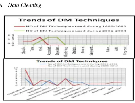
[image:2.595.314.552.566.746.2]A. Data Cleaning
In this section, we look at the cleaning techniques involved in order to check if any incomplete data (missing out on attribute values), noisy (containing errors and outliers that extend away from the expected values) and inconsistent (mismatches of data stored in various formats) data exists. The kinds of errors that are encountered are:
Incomplete Data
Noisy Data
Inconsistent Data
Data cleaning routines involve cleaning the data by filling up the missing values, identifying and removing any outliers, smoothening noisy data and finding solutions for inconsistent data.
Dirty Data often poses a challenge when it comes to training the model, as the model cannot be trained with wrong or inaccurate data as well as keeping the fact in mind that the over fitting of data with the function being modelled.
a. Data Cleaning For Incomplete Data/Missing Values. The missing data problem states emptiness of attributes while filling up data (for example, in this case, students may not have cleared an examination which was a part of the course or results for that particular re-evaluation may not have been recorded and may have been overlooked) and also as the model cannot be trained on missing values, following steps have to be taken:
Ignore the tuple: This usually is used when the attribute label or description itself lacks out on a lot of attribute values, then the tuple can be ignored/deleted and will not be considered as a metric for the values. If it’s less significant and if the variation of data across different attributes is of considerable size, then this method proves to be inefficient. Fill in the missing value: Here the attributes that are missing have to be filled in manually by going through collection techniques again for recollecting the data that have been missed out. However, this task/routine is very time consuming and cannot be used when very large datasets are involved.
Use a global constant: In this technique, we can assign the same constant values to different missing attributes, so that those fields aren’t left out. However the mining program may find this confusing as the same constant has been assigned to different fields and the program may figure out an incorrect pattern out of this.
Use the attribute mean: Calculate the average or mean value of attributes and replace the attribute value with this mean.
Usage of the attribute mean values for samples belongs to the same.
Use the most probable value: By making use of Bayesian’ formulas or Decision Trees to get an inference.
b. Data Cleaning For Noisy Data.
Noisy Data involves data that have random errors or has a value that deviates from what was expected of it. The following steps have to be taken:
Binning Methods. Binning methods generally make use of the neighboring values of the noisy values. The sorted data values are then put into different bins on the basis of local smoothing principle.
Clustering: Outliers in a given data and algorithm may be detected by clustering when the values are organized into clusters.
Human and Computer Inspection: Outliers can be identified through this technique as outliers are informative (you can identify exceptions). Patterns whose surprise content is above a minimum threshold values are listed. Thereafter humans have to sort the required patterns to identify garbage ones.
Regression.Is one of the most useful techniques when it comes to smoothening noisy data, where lines/multidimensional surfaces can be used to best fit 2 or more variables (Linear/Multiple Linear Regression) such that any of these variables can be used to predict another value. Data Cleaning For Inconsistent Data.
Inconsistency in data can be reduced by checking out functional dependencies between variables (attributes) and mainly consists of removing redundant data. Data validation tools can be put in placeso as to check data violations. For mistakes made at entry level, a paper trace can be done and routines established so as to check such violations in the future.
A. Data Integration
Since the data has been collected from multiple records it has been recorded into one single sheet, as multiple mark sheets were involved and that comprises the dataset that the model will train on (after preprocessing is done). Redundancies have to be eliminated so as to provide a simpler, clearer and concise version of the dataset.
B.Data Transformation
In this section, we will learn different techniques to transform data by consolidating it into appropriate format for mining. Some of the techniques used are:
Normalization. The attributed data is scaled so as to fall within a small specified range of data.
Smoothing. Outliers are resolved and the methods involve:
Binning
Clustering
Regression
Aggregation. The data is summarized and a data cube is constructed for the data at different granularities.
Generalization of Data. The low level or primitive data are mapped to higher level concepts through the concept hierarchy.
C. Data Reduction
In this section, we strive to reduce attributes in case, it’s of a larger number, so that we get ample metrics that serve the purpose of getting good analytical results as well as the data set being efficient. This strives to reduce time constraint on the algorithm making complex data analysis. The following techniques are used:
Data Cube Aggregation. Aggregation is applied on the data values which transforms it into construction of a data cube(an OLAP technique).
Data Compression. We reduce the standard data set size. The methods use for this are:
Principal Component Analysis: Is a statistical procedure which make use of an orthogonal that will convert it to a set of observations of possibly correlated variables into a set of values of linearly uncorrelated variables called principal components.
Wavelet Transform: The representation of a square-integrable(may be real- or complex-valued ) function by a certain orthonormalseries is called a wavelet series which are generated by a wavelet.
Numerosity Reduction. Data is replaced by using parametric models(such as regression) or non-parametric methods includes clustering and sampling(the selection of a subset).
Discretization & Concept Hierarchy. Lower level attributes are mapped to higher level attributes or are replaced by ranges as well and allows mining at multiple levels of abstraction
V. DATA VISUALIZATION
In this section, we look at different techniques/methods that encode numerical data using dots, lines or bars to present the statistics in a visual way or a way where it is more
interpretable, in order to convey the idea and to provide visual insights into sparse and complex data sets in an intuitive way.
A. Characteristics of Graphical Displays:
It shows the results of the data.
Induce the viewer to think about the substance rather than about methodology, graphic design, and the technology of graphic production or something else.
Avoid distorting what the data has to say.
Present many numbers in a small space.
Encourage the eye to compare different pieces of data.
Make large data sets coherent.
Reveal the data at several levels of detail, from a broad overview to the fine structure.
Serve a reasonably clear purpose: Description, Exploration, Tabulation or Decoration.
Be closely integrated with the statistical, analytical and verbal descriptions of a data set.
B. Types of Quantitative Messages
1) Quantitative Message are used for helping
communicate the data, they take the numerical form (in visual data representations). The various quantitative message formats are as follows:
Time-series. A single variable that is captured over a period of time. A line chart may be used to demonstrate the trend.
Ranking. Categorical subdivisions are ranked in ascending or descending order during a single period. A bar chart may be used to show the comparison across the sales persons.
Part-to-whole. Categorical subdivisions are measured as a ratio to the whole. A pie chart or bar
chart can show the comparison of ratios, such as the market share represented by competitors in a market.
Deviation. Categorical subdivisions are compared against a reference, for a given time period. A bar chart can show comparison of the actual versus the reference amount.
Frequency distribution. Shows the number of observations of a particular variable for given interval. A histogram, a type of bar chart, may be used for this analysis. A box plot helps visualize key statistics about the distribution, such as median, quartiles, outliers, etc.
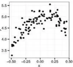
Correlation. Comparison between observations represented by two variables (X,Y) to determine if they tend to move in the same or opposite directions. A scatter plot is typically used for this message.
Nominal comparison.Comparing categorical subdivisions in no particular order, such as the sales volume by product code. A bar chart may be used for this comparison.
Geographic or geospatial.Comparison of a variable across a map or layout, such as the unemployment rate by state or the number of persons on the various floors of a building. A cartogram is a typical graphic used.
C. Types Terminologies.
Categorical: Text labels describing the nature of the data, such as "Name" or "Age". This term also covers qualitative (non-numerical) data.
Quantitative: Numerical measures, such as "25" to represent the age in years.
[image:4.595.377.502.498.613.2]Data Visualization Representations.
Figure 2: Basic scatterplot of two variables
Visual Dimensions.
X Position and Y Position
(Symbol/Glyph)
Figure 3: A bar graph
Visual Dimensions.
Length/Count
Category
(Color)
Figure 4: A histogram Visual Dimensions.
a.Bin Limits b.Count/Length c(Colour)
Figure 5: Network Analysis Visual Dimensions
Nodes Size
Nodes Colour
Ties Thickness
Ties Colour Spatialization
VI. CONCLUSION
This paper is presented with an intention to introduce all the necessary terms and techniques that are required to start with Educational Data Mining (EDM). This paper discusses all methods right from data capturing, data cleaning, applying different data mining techniques to the cleaned data, to gain insights and finally making the insights more illustrative and interactive by using different tools of data visualization. Analysts can choose any of these methods that match the scope of their analysis. We strongly hope this paper serves the best purpose for people interested in EDM.
REFERENCES
[1]. (Ahmed, A.B.E.D. and Elaraby, I.S., 2014. Data Mining: A prediction for Student's Performance Using Classification Method. World Journal of Computer Application and Technology, 2(2), pp.43-47
[2]. S.N. Madhu, N. Madhu, ―Discovery of students’ academic patterns using data mining techniques‖ International Journal of Computer Science and Engineering, Vol 4, no. 06, 2012.
[3]. [Bhardwaj, B.K. and Pal, S., 2012. Data Mining: A prediction for performance improvement using classification. (IJCSIS) International Journal of Computer Science and Information Security, Vol. 9, No. 4, April 2011.
[4]. Ramaswami and R. Bhaskaran, ―A Study on Feature Selection Techniques in Educational Data Mining,‖ J. Comput., vol. 1, no. 1, pp. 7–11, 2009.
[5]. Pandey, U.K. and Pal, S., 2011.Data Mining: A prediction of performer or underperformer using classification. (IJCSIT) International Journal of Computer Science and Information Technologies, Vol. 2 (2), 2011, 686690.
[6]. V. Kumar, ―An Empirical Study of the Applications of Data Mining Techniques in Higher Education,‖ Int. J. Adv. Comput.Sci. Appl., vol. 2, no. 3, pp. 80–84, 2011.
[7]. M. Swamy and M. Hanumanthappa, ―Predicting academic success from student enrolment data using decision tree technique,‖ Int. J. Appl. Inf. Syst., vol. 4, no. 3, pp. 1–6, 2012.
[8]. Amjad Abu Saa ,‖Educational Data Mining & Students’ Performance Prediction‖, International Journal of Advanced Computer Science and Applications, Vol. 7, No. 5, 2016.