A novel differential evolution for model order reduction

(1)

840

A novel differential evolution for model order reduction

Raghav Prasad Parouha

Department of Mathematics, Indira Gandhi National Tribal University Amarkantak M.P. India Email id: [email protected]

Abstract- Many variants of Differential Evolution (DE) algorithms exist in literature to solve Engineering Design Problems. However, the performance of DE is highly affected by the inappropriate choice of its operators like mutation and crossover. Moreover, in general practice, DE does not employ any strategy of memorizing the so-far-best results obtained in the initial part of the previous cycle. In this paper a „Memory based DE (MBDE)‟ propose which having two „swarm operators‟. These operators are based on the personal and global best mechanism of particle swarm optimization (PSO). Proposed MBDE is validate on 13 typical benchmark functions. Further to test its efficacy five different model order reduction (MOR) problems for single-input and single-output system are solved by MBDE. The results of MBDE are compared with state-of-the-art algorithms that also solved those problems. Numerical, statistical and graphical analysis reveal the competency o f the proposed algorithm.

Index Terms-Differential Evolution, Mutation, Crossover, Engineering design problems.

1. INTRODUCTION

Nowadays, optimization problems are very important and frequently appear in the real world. Solving such problems is a challenging area of research in the science and engineering disciplines. In spite of many Evolutionary Algorithms (EAs), Differential Evolution (DE) [1] is an efficient, formidable and popular ingredient. The DE has many advantages like easy implementation, reasonably faster, robust and exhibits effective global search ability [2-8]. In general, it also has efficient global search ability and hence considered as global optimization algorithm [9]. Therefore, it has been applied to solve many engineering optimization problems such as mechanical engineering design problem [10], fuzzy clustering of image pixel [11], economic load dispatch [12], nuclear reactor core design [13] and many others [9]. However, most of the time, the solution gets stacked in some local optima. As a result, it leads to a premature convergence. It is because of DE have some individual shortcomings like sometimes the solution gets stacked in local optimum which leads to premature convergence [8, 14, 15]. Also, same as other EAs, DE does not guarantee to reach at global optimal solution in a finite time interval [8]. Therefore, in order to improve the performance of basic DE, a number of attempts are made in the literature [2-23]. A detailed survey on the variants of DE can be found in [20, 21]. Moreover, in order to improve the robustness of DE, a number of mutation strategies of DE have been proposed in [9, 16, 17, 19, 20, 21, 22]. Basically, DE is much sensitive to choice of the mutation strategy. Also, it is very difficult to recommend a fixed set of parameters for different problems [9, 16, 17, 19, 20, 21, 22]. On the other hand, inappropriate choice of mutation strategy may lead to premature convergence, stagnation or wastage of computational time [9].

Similarly, researchers mainly used two types of crossover schemes in DE namely binomial crossover and exponential crossover [1]. In [24], Price recommended the use of binomial crossover is better.

But later, it is observed that there are no significant differences between these crossovers [25].

Unfortunately, according to „No Free Lunch Theorem [26])‟, no single optimization method exist which is able to solve consistently to all global optimization problems. In spite of quite a good number of DE variants exist in the literature; DE further yields improved results while hybridizing with Particle Swarm Optimization (PSO) [27]. Each of them is capable of dominating the shortcoming of the other to add the robustness in the resultant hybrid algorithm. The magical synergy of DE and PSO has been well established and has crossed many success milestones in recent past. Yet, many hybrid methods of DE and PSO have been proposed [28-46]. These approach moves around the enhancement of capabilities of DE and PSO in various aspects and successfully applied to wide range of optimization problems such as medical image processing problem [30], engineering design optimization [37, 38], well placement optimization [40], power systems optimization [41], digital FIR filter design [42] and many others.

(2)

841 Inspired by above fact a memory based differential

evolution proposed in this paper where two novel operators (swarm mutation and swarm crossover) were introduced under the PSO environment. The reminder of this paper is organized as follows. Section 2 presents overview of the basic DE. Section 3 presents a detailed description of the proposed algorithm. The efficiency of the proposed algorithm is validated through unconstrained benchmark functions in Section 4. The proposed algorithm is applied to solve MOR problems in Section 5. Section 6 draws the conclusion of the paper along with some highlights on future scopes.

2. OVERVIEW OF BASIC DIFFERENTIAL EVOLUTION

Differential Evolution (DE) is an Evolutionary Algorithm (EA) proposed by Storn and Price in 1995 [1]. The outline of the classical DE may be given as follows.

Initialization

Initialize a population of NP target vectors (parents)

( ) , is randomly

generated within user-defined bounds, where D is the dimension of the optimization problem.

Mutation

Let ( ) ( ) ( ) ( ) be the „ ‟

individuals at „ _{‟ generation. A mutant vector}

( ) ( ( ) ( ) ( )) is generated as follows.

( ) ( ( ) ( ))

where, [ ] is the mutation factor.

Crossover

The target vector ( ) and the mutant vector (

) create a new trial vector ( ) ( ( ) ( ) ( )) as follows.

( )

{ ( ) ( ) ( ) ( ) ( ) ( )

where ( ) ( ), [ ] is the crossover constant.

Selection

Selection operates by comparing the individual‟s fitness to generate the next generation population.

( )

{ ( ) ( ( )) ( ( )) ( )

The cyclic implementation of mutation, crossover and selection is continued till it meets with the pre-defined stopping criterion.

3. PROPOSED METHOD

Motivated by the advantages and disadvantages of DE, and above observations, in this present study „Memory Based Differential Evolution (MBDE)‟ proposed. where the mutation and crossover are termed as „swarm mutation‟ and „swarm crossover‟

because of these operator based on and mechanism of PSO [27]. The proposed operators are explained in the following section.

3.1.Swarm mutation

Let ( ) ( ) ( ) ( ) is the target

vector and ( ) is the personal best position vector, in the current generation „ ‟. Then a mutant vector (i.e. perturbed vector) ( ) ( ) ( ) ( ) is

generated by „Swarm Mutation‟ as follows.

( )

( ) | (

_{( ))}

( _{( ))}| (

_{( )}_{( ))}

| (

_{( ))}

( _{( ))}| (

_{( )}_{( ))}₍₁₎

where ( ) is the personal and ( ) is the global best position of the vector ( ) respectively,

( ( )) is the personal best and ( _{( ))}_is

the global best function value of the vector ( )

respectively, ( _{( ))}_{is the worst function value}

of vector ( ), in the current generation „ ‟. Whenever ( _{( ))}_{it will be replaced by a}

large positive constant „ ‟, in order to impact a small perturbation to ( ). Clearly, each of the ratio-coefficient of the terms ( _{( )}_{( ))}_and

( _{( )}_{( ))}_{generates a real constant factor}

between [ ]_{that controls the amplification of the}

differential variation.

3.2.Swarm crossover

To generate a new trial vector ( ) ( ) ( ) ( ), „Swarm Crossover‟ works

as follows.

( )

{

( ) ( ) ( ( ) ( )) ( ) ( ) ( ) ( ) ( _{( )} _{( ))}

( ) ( )

(2)

where ( ) is the mutant vector, ( )is the target vector, ( ) ( ), [ ] is the crossover constant.

3.3.Steps of proposed algorithm

Steps of the proposed MBDE presented below. Step 1: Randomly generate all vectors i.e. ( )

( ) in the prescribed search

range

Step 2: Evaluate ( ); i. e. find the function values of

( ) for i = 1, 2, …, NP

(3)

842

Step 7: Swarm Mutation using the Eq. (1) Step 8:Swarm Crossover using the Eq. (2) Step 9: Apply Elitism

Step 10: Stop if the termination criterion is met, else set t = t + 1 and go to Step-5

4. VALIDATION OF PROPOSED ALGORITHM

In this section before solving the MOR problem, proposed MBDE applied to solve 13 unconstrained benchmark functions (reported in Table 1 and taken from [23]).

Table 1 Benchmark Functions

f Function Name Formulation S C fmin

f12 Penalized

1

f13 Penalized2

1

S: domain of the variables, fmin: Global minima, C: Function characteristics, U: Unimodal, M: multimodal, S: separable, N: non-separable

Table 2 Comparison of MBDE with others in [23] for 13 (10D) benchmark functions, in terms of mean and S. D. of the best objective function value

f Max. NFEs Algorithm

MBDE GDE DE/rand/1 DE/best/1 DE/target-to-best/1

f1 100000

f7 100000 _(2.420e-08)1.037e-006

1.329e-03

f10 100000 _(0.000e+00)1.284e-015

(4)

843

f13 100000 _(2.042e-48)1.346e-032

1.349e-32

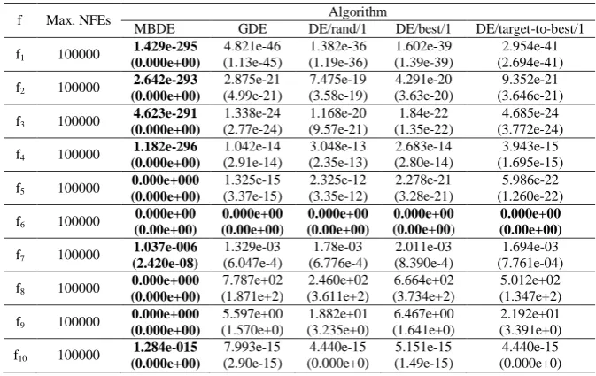
Table 3 Comparison of MBDE with others in [23] for 13 (30D) benchmark functions, in terms of mean and S. D. of the best objective function value

The

simulations were conducted on Intel(R) Core-i3, 2.20 GHz, 2GB RAM, computer in the C-Free Standard 4.0 Environment. To execute the performance of MBDE, population size (NP) is taken as 10D and 30D (where D is the dimensions of the problems) and after fine-tuned crossover rate are recommended as CR = 0.9 for further study. stopping criterion in this study remains the same as in GDE [23]. The results produced by MBDE on 13 typical unconstrained benchmark functions have been

compared with state-of-the-art algorithms.

4.1.Numerical analysis

The mean and standard deviation (S.D.) of the best objective function value for 50 runs is reported in Table 2 and Table 3 for 10D and 30D benchmark functions, respectively. The results produced by proposed algorithm are compared with DE/rand/1, DE/best/1, DE/target-to-best/1 and group based differential evolution (GDE) [23]. It is observed that from Table 2 and Table 3 that MBDE outperforms its competitors in all benchmark functions both for 10D and 30D. Only for f6, MBDE performs equally to

others for 10D, but better than others in 30D except GDE. It is worth noting that in almost all cases MBDE impacts very less S. D.

f Max. NFEs Algorithm

MBDE GDE DE/rand/1 DE/best/1 DE/target-to-best/1

f1 300000

f13 300000 _(1.038e-30)1.642e-023

(5)

844

Fig. 1(a). Average NFEs of MBDE with others in [23] for 13 (10D) benchmark Functions

Fig. 1(b). Average NFEs of MBDE with others in [23] for 13 (30D) benchmark Functions

The average numbers of function evaluations (NFEs) for all the algorithms under consideration are compared in Fig. 1(a) and 1(b) for 10D and 30D, respectively. From these figure it can be concluded that MBDE uses fewer number of NFEs compared to rest algorithms.

4.2.Convergence analysis

The convergence speed of MBDE is compared with the other algorithms reported in [23] over a set of

5 higher dimensional (30D) typical test functions (Sphere, Rosenbrock, Schwefel, Rastrigin and Ackley) are picked. The convergence graphs are presented in Fig. 2(a-e). Form these figures it can be concluded that in all the functions MBDE converge much faster than other algorithms. It can be concluded that, MBDE is greatly stable to minimize the unconstrained optimization problems.

Fig. 2(a). Convergence of MBDE with others in [23] for Sphere Function (30D)

Fig. 2(b). Convergence of MBDE with others in [23] for Rosenbrock Function (30D)

Fig. 2(c). Convergence of MBDE with others in [23] Fig. 2(d). Convergence of MBDE with others in [23]

(6)

845 for Schwefel Function (30D) for Rastrigin Function (30D)

Fig. 2(e). Convergence of MBDE with others in [23] for Ackley Function (30D)

4.3.Statistical analysis

To compare the performance of multiple algorithms on the test suite, a well-known ranking based test namely Friedman test [47] is selected. In Table 4 the average ranking of MBDE, GDE, DE/rand/1, DE/best/1, DE/target-to-best/1 on unconstrained benchmark functions are presented.

Table 4 Average rankings achieved by Friedman test

Algorithms Ranking

MBDE 5.18

GDE 4.27

DE/rand/1 2.26 DE/best/1 3.05 DE/target-to-best/1 3.57

The performance of the compared algorithms can be sorted by average ranking into the following order: MBDE, GDE, DE/target-to-best/1, DE/best/1, DE/rand/1. The best average ranking was obtained by the proposed MBDE, which outperforms the other algorithms.

5. APPLICATION OF PROPOSED ALGORITHM

In this section proposed MBDE is applied to solve the model order reduction (MOR) problem. A brief description of the MOR problem is presented below.

5.1.Problem statement

Let‟s consider a nth order linear time invariant dynamic single-input and single-output system (SISO) system given as follows.

( ) ( )

( ) ∑

∑ (3)

Where and are known constants. The problem is to find out order reduced model in the transfer function form ( ), where represented by Eq. (4) such that the reduced model retains the important characteristics of the original system and

approximates its step responses as closely as possible for the same type of inputs with minimum Integral square error (ISE) as well as Impulse response energy(IRE).

( ) ( )

( ) ∑

∑ (4)

where and are unknown constants.

Mathematically, the ISE of step responses of the original and the reduced system can be expressed by the following error index given by Eq. 5).

∫ [ ( ) ( )] (5) where ( ) is the unit step response of the original system and ( ) is the unit step response of the reduced system. The error index is the function of unknown coefficients of reduced order model so that the error index is minimized.

The IRE for the original and the various reduced models is given by as following Eq. (6).

∫ ( ) (6) where, ( ) is the Impulse response of the system. In this paper the objective is to minimize the objective function based on both ISE and IRE.

5.2.Procedure to reduced second order model

for the given higher order system

Let‟s consider the original high order system transfer function is given by Eq. (7).

( )

(7)

where is the order of the system and .

( )

( )( )( ) ( ) (8)

where are

distinct real Eigen values of the system. The unit step responses of (8) can be determined as follows.

( ) ( )

(9) where are real constants. Taking inverse Laplace transformation of Eq. (9),

( )

10)

0 5 10 15 20 25 30 35 40 45 50

0.0 2.0x100 4.0x100 6.0x100 8.0x100 1.0x101 1.2x101 1.4x101 1.6x101 1.8x101 2.0x101 2.2x101

DE/rand/1 DE/best/1 DE/target-to-best/1 GDE

MBDE Ackley Function

O

b

je

cti

ve

F

u

n

cti

o

n

Va

lu

e

(7)

846 where is steady state response and the rest of the

terms are transient response of the system given in equation (8). Let the proposed reduced order system constructed is of 2nd order, where

( ) condition should be fulfilled.

(14) The ISE of the transient responses of the system of (8) and (11) is given as follows. unknown constants, which are randomly generated in

MBDE and the value of are calculated. The reduced model ( ) is obtained over 30 independent runs so that the integral square error is minimized. In the next step that reduced model ( ) is taken where IRE given by Eq. (6) is also minimized.

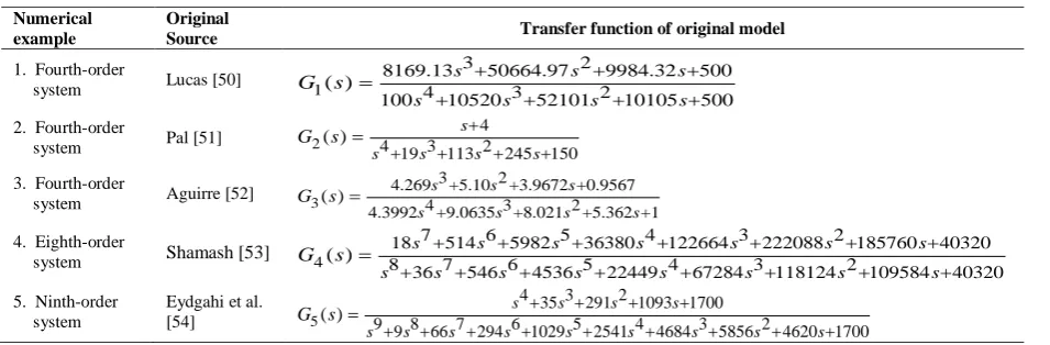
5.3.Simulations results and discussion

In order to assess the efficiency of the proposed MBDE, it has been applied on five numerical examples of MOR problems. These numerical examples are reported in Table 5, having real and distinct Eigen values. Proposed MBDE aims at solving these numerical examples with two objectives. They are (i) to minimize the Integral Square Error (ISE) and (ii) Impulse Response Energy (IRE); between original higher order system and reduced lower order system.

The result produced by MBDE for considered five test system is compared with FBDE [18], LICLDE [48] and ABC [49]. For the fair comparison, the population

size, independent runs and stopping criterion are same as LICLDE [48]. Remaining parameters of MBDE are same as section 4. The best reported ISE and IRE are boldfaced in the respective tables. The original and the reduced systems for numerical examples 1, 2, 3, 4 and 5 are presented in Tables 6, 7, 8, 9 and 10, respectively.

Table 5 List of 5 numerical example of Model Order Reduction (MOR) problem

Numerical example

Original

Source Transfer function of original model

1. Fourth-order

system Lucas [50] 1

3 2

8169.13 50664.97 9984.32 500

4 3 2

100 10520 52101 10105 500

( ) s s s

s s s s

G s   

   



2. Fourth-order

system Pal [51] 2

3. Fourth-order

system Aguirre [52] 3

3 2

4.269 +5.10 +3.9672 +0.9567

4 3 2

4.3992 +9.0635 +8.021 +5.362 +1

( ) s s s

s s s s

G s 

4. Eighth-order

system Shamash [53] 4

7 6 5 4 3 2

18 514 5982 36380 122664 222088 185760 40320

8 ₃₆ 7 ₅₄₆ 6 ₄₅₃₆ 5 ₂₂₄₄₉ 4 ₆₇₂₈₄ 3 ₁₁₈₁₂₄ 2 ₁₀₉₅₈₄ ₄₀₃₂₀

Table 6 Comparison of proposed method with existing methods for numerical example 1

Method of reduction Reduced Models R s₁( ) ISE IRE

FBDE [18] ₂85.33529245 462.3004006

113.6582937 462.3004006

s

s s



(8)

847

LICLDE [48] 2

101.3218182 867.893179

169.4059231 867.893179

s

s s



  0.0036228741 34.069918

ABC [49]

2

485 +50000

+4187 +50000

s

s s

0.011624954 34.065841

Method of reduction Reduced Models R₂( )s ISE IRE

Original G₂( )s --- 0.00026938

MBDE

2

-0.0045958 0.08260527

4.021015 3.0988975

s

s s



  4.001259e-006 0.0002699

LICLDE [48]

2

0.0195 0.2884

14.9813 10.82

s

s s

 

  4.3168e-006 0.00027

ABC [49]

2

0.0318 +4.0074

+13.7409 +150.2775

s

s s

0.0005 0.0039

Method of reduction Reduced Models R s₃( ) ISE IRE

Original G s3( ) --- 0.54536

MBDE

2

0.75984 2.94328

3.15286 3.079858

s

s s



  0.21501e-01 0.545388

LICLDE [48]

2

0.7853 +2.949

+3.1515 +3.0823

s

s s

0.338 e−01 0.54538

ABC [49]

2

0.2034 +8.994

+7.9249 +9.4008

s

s s

0.03501 0.54552

Method of reduction Reduced Models R s₄( ) ISE IRE

Original G4( )s --- 21.740

MBDE 14.886587₂ 4.78524

5.98827 4.78524

s

s s



  0.08e-03 21.74

FBDE [18]

2

17.32178 5.3660

7.0240 5.3660

s

s s



  0.80e-03 21.74

LICLDE [48]

2

17.203 5.3633

6.9298 5.3633

s

s s



  0.80e-03 21.74

ABC [49] ₂17.387 +5.3743

+7.091 +5.3743

s

s s 0.00085 21.696

Method of reduction Reduced Models R s₅( ) ISE IRE

Original G5( )s --- 0.47021

MBDE

2

0.598856818 0.9965860

1.49989469 0.9965860

s

s  s

 

0.20595e-01 0.471842

LICLDE [48]

2

-0.6372 +1.0885

+1.5839 +1.0885

s

s s

(9)

848

Fig. 3(a). Comparison of step response for numerical example 1

Fig. 3(b). Comparison of impulse response for numerical example 1

Fig. 4(a). Comparison of step responses for numerical example 2

Fig. 4(b). Comparison of impulse responses for numerical example 2

(10)

849

The unit step responses of the original, the reduced systems using MBDE and best reported method in [18, 48, 49] are shown in Figs. 3(a), 4(a), 5(a), 6(a) and 7(a), respectively for corresponding numerical examples. Also the impulse responses of the original, the reduced systems using MBDE and best reported reduced models obtained by MBDE are closest to that of the originals. Moreover, the step response (Figs. 3(a), 4(a), 5(a), 6(a) and 7(a)) as well as impulse response curve (Figs. 3(b), 4(b), 5(b), 6(b) and 7(b)) seem to be closely lying on the original curve. It may also be seen that the steady state responses of the original and the reduced order models by MBDE are exactly matching while the transient response

matching is also very close as compared to other methods. Thus these numerical examples establish the superiority of MBDE over other methods. Finally, MBDE performance is superior to state-of-the-art algorithms. Thus, MBDE may be treated as a robust method to solve MOR problem.

6. CONCLUSION AND FUTURE WORKS

In this paper a „Memory Based Differential Evolution (MBDE)‟ is proposed for solving model order reduction problems. It employs two new operators (swarm mutation and swarm crossover) based on PSO environment. The performance of MBDE has been compared with state-of-the-art variants of DE and other recent algorithms.

(11)

850 respect to minimize the considered engineering

optimization problem, achieves a marginal improvement over others.

As a future works, MBDE can be applied in large real world problem and engineering and for solving multi-objective optimization problems.

REFERENCES

[1] R. Storn and K. Price, “Differential evolution – a simple and efficient adaptive scheme for global optimization over continuous spaces”, Journal of Global Optimization, vol. 11, no. 4, pp. 341–359, 1997.

[2] H.Y. Fan and J. Lampinen, “A trigonometric mutation operation to differential evolution”, Journal of Global Optimization, vol. 27, no.1, pp. 105–129, 2003.

[3] O. Hrstka and A. Kucerova, “Improvement of real coded genetic algorithm based on differential operators preventing premature convergence”, Advances in Engineering Software, vol. 35, no. 3-4, pp. 237–246, 2004. [4] S. Das, A. Konar and U.K. Chakraborty, “Two

improved differential evolution schemes for faster global search”, In: Proceedings of the 2005 Conference on Genetic and Evolutionary Computation, pp. 991–998, 2005.

[5] J. Liang, A. Qin, P. Suganthan and S. Baskar, “Comprehensive learning particle swarm optimizer for global optimization of multimodal functions”, IEEE Transactions on Evolutionary Computation, vol. 10, no. 3, pp. 281–295, 2006.

[6] F. Z. Huang, L. Wang and Q. He, “An effective co-evolutionary differential evolution for constrained optimization”, Applied Mathematics and Computation, vol. 186, no. 1, pp. 340–356, 2007.

[7] S. Rahnamayan, H. R. Tizhoosh and M. M. A. Salama, “Opposition-Based Differential Evolution”, IEEE Transactions on Evolutionary Computation, vol. 12, no. 1, pp. 64–79, 2008. [8] S. Das, A. Abraham, U. K. Chakraborty and A.

Konar, “Differential evolution using a neighborhood-based mutation operator”, IEEE Transactions on Evolutionary Computation, vol.13, no. 3, pp. 526–553, 2009.

[9] K. V. Price, R. M. Storn and J. A. Lampinen, “Differential Evolution: A Practical Approach to Global Optimization”, Berlin: Springer, 2005.

[10] M. Zhang, W. Luo and X. Wang, “Differential evolution with dynamic stochastic selection for constrained optimization”, Information Sciences, vol. 178, no. 15, pp. 3043–3074, 2008.

[11] S. Das and S. Sil, “Kernel-induced fuzzy clustering of image pixels with an improved

differential evolution algorithm”, Information Sciences, vol. 180, no. 8, pp. 1237–1256, 2010. [12] Y. Wang, B. Li and T. Weise, “Estimation of distribution and differential evolution cooperation for large scale economic load dispatch optimization of power systems”, Information Sciences, vol. 180, no. 12, pp. 2405–2420, 2010.

[13] W.F. Sacco and N. Henderson, “Differential evolution with topographical mutation applied to nuclear reactor core design”, Progress in Nuclear Energy, vol. 70, pp. 140–148, 2014. [14] N. Noman and H. Iba, “Accelerating

differential evolution using an adaptive local search”, IEEE Transactions on Evolutionary Computation, vol. 12, no. 1, pp. 107–125, 2008.

[15] J. Lampinen and I. Zelinka, “On stagnation of the differential evolution algorithm”, In: Proceedings of MENDEL 2000, 6th International Mendel Conference on Soft Computing, pp. 76–83, 2000.

[16] E. Mininno and F. Neri, “A memetic differential evolution approach in noisy optimization”, Memetic Computing, vol. 2, no. 2, pp. 111–135, 2010.

[17] R. Mallipeddi, P. Suganthan, Q. Pan and M. Tasgetiren, “Differential evolution algorithm with ensemble of parameters and mutation strategies”, Applied Soft Computing, vol. 11, no. 2, pp. 1679–1696, 2011.

[18] H. Sharma, J. Bansal and K. Arya, “Fitness based differential evolution”, Memetic Computing, vol. 4, no. 4, pp. 1–14, 2012. [19] W. Gong and Z. Cai, “Differential evolution

with ranking based mutation operators”, IEEE transaction on Systems Man and Cybernetics Part B- Cybernetics, vol. 43, no. 6, pp. 2066– 2081, 2013.

[20] F. Neri and V. Tirronen, “Recent advances in differential evolution: a survey and experimental analysis”, Artificial Intelligence Review, vol. 33, no. 1-2, pp. 61–106, 2010. [21] S. Das and P.N. Suganthan, “Differential

evolution: a survey of the state-of-the-art”, IEEE Transactions on Evolutionary Computation, vol. 15, no. 1, pp. 4–31, 2011. [22] Qin, V. Huang and P. Suganthan, “Differential

evolution algorithm with strategy adaptation for global numerical optimization”, IEEE Transactions on Evolutionary Computation, vol. 13, no. 2, pp. 398–417, 2009.

[23] M. F. Han, S. H. Liao, J. Y. Chang and C. T. Lin, “Dynamic group-based differential evolution using a self-adaptive strategy for global optimization problems”, Applied Intelligence, vol. 39, no. 1, pp. 41-56, 2013. [24] K. V. Price, “An Introduction to Differential

(12)

851 and Fred Glover, editors, New Ideas in

Optimization, McGraw-Hill, London, pp. 79– 108, 1999.

[25] K. Price and R. Storn, “http://www.icsi.berkeley.edu/~storn/code.html ”, website as in August 2008.

[26] D. H. Wolpert and W. G. Macready, “No Free Lunch Theorems for Optimization”, IEEE Transactions on Evolutionary Computation, vol. 1, no. 1, pp. 67-82, 1997.

[27] J. Kennedy and R. C. Eberhart, “Particle Swarm Optimization”, In: Proceeding of IEEE International Conference on Neural Networks, pp.1942–1948, 1995.

[28] T. Hendtlass, “A combined swarm differential evolution algorithm for optimization problems”, Lecture Notes Computer Science, Springer Verlag, vol. 2070, pp. 11-18, 2001. [29] W. J. Zhang and X. F. Xie, “DEPSO: Hybrid

particle swarm with differential evolution operator”, in: proceedings IEEE International Conference Systems Man Cybernetics, vol. 4, pp. 3816-3821, 2003.

[30] H. Talbi and M. Batouche, “Hybrid particle swarm with differential evolution for multimodal image registration”, in: proceedings of the IEEE International Conference on Industrial Technology, vol. 3, pp. 1567–1573, 2004.

[31] S. Das, A. Konar and U. K. Chakraborty, “Improving particle swarm optimization with differentially perturbed velocity”, in: proceedings Genetic Evolutionary Computation Conference, pp. 177-184, 2005.

[32] P. W. Moore and G. K. Venayagamoorthy, “Evolving digital circuit using hybrid particle swarm optimization and differential evolution”, International Journal of Neural Systems, vol. 16, no. 3, pp. 163-177, 2006.

[33] Z. F. Hao, G. H. Guo and H. Huang, “A particle swarm optimization algorithm with differential evolution”, in: proceedings sixth International Conference Machine Learning and Cybernetics Hong Kong China, pp. 1031-1035, 2007.

[34] S. Das, A. Abraham and A. Konar, “Particle swarm optimization and differential evolution algorithms: technical analysis, applications and hybridization perspectives”, Advances of Computational Intelligence in Industrial Systems, Studies in Computational Intelligence, Springer Verlag, Germany, pp. 1– 38, 2008.

[35] C. Zhang, J. Ning, S. Lu, D. Ouyang and T. Ding, “A novel hybrid differential evolution and particle swarm optimization algorithm for unconstrained optimization”, Operations Research Letters, vol. 37, no. 2, pp. 117–122, 2009.

[36] X. Wang, Q. Yang and Y. Zhao, “Research on hybrid PSODE with triple populations based on multiple differential evolutionary models”, in: proceedings International Conference Electrical Control Engineering Wuhan China, pp. 1692-1696, 2010.

[37] H. Liu, Z. X. Cai, and Y. Wang, “Hybridizing particle swarm optimization with differential evolution for constrained numerical and engineering optimization”, Applied Soft Computing, vol. 10, no. 2, pp. 629-640, 2010. [38] A. E. Dor, M. Clerc and P. Siarry,

“Hybridization of Differential Evolution and Particle Swarm Optimization in a new algorithm DEPSO-2S”, Swarm and Evolutionary Computation, vol. 7269, pp. 57-65, 2012.

[39] B. Xin, J. Chen, J. Zhang, H. Fang and Z. Peng, “Hybridizing differential evolution and particle swarm optimization to design powerful optimizers: a review and tax-onomy”, IEEE Transactions on Systems Man and Cybernetics Part C: Applications and Reviews, vol. 42, no. 5, pp. 744–767, 2012.

[40] E. Nwankwor, A. Nagar and D. Reid, “Hybrid differential evolution and particle swarm optimization for optimal well placement”, Computational Geosciences, vol. 17, no. 2, pp. 249-268, 2013.

[41] S. Sayah and A. Hamouda, “A hybrid differential evolution algorithm based on particle swarm optimization for nonconvex economic dispatch problems”, Applied Soft Computing, vol. 13, no. 4, pp. 1608–1619, 2013.

[42] Vasundhara, D. Mandal, R. Kar and S. P. Ghoshal, “Digital FIR filter design using fitness based hybrid adaptive differential evolution with particle swarm optimization”, Natural Computing, vol. 13, no. 1, pp. 55-64, 2014.

[43] K. N. Das and R. P. Parouha, “An ideal tri-population approach for unconstrained optimization and applications”, Applied Mathematics and Computation, vol. 256, pp. 666-701, 2015.

[44] R. P. Parouha and K. N. Das, “Parallel hybridization of Differential Evolution and Particle Swarm Optimization for constrained optimization with its application”, International Journal of Systems Assurance Engineering and Management, vol. 7, no. 1, pp. 143–162, 2016. [45] K. N. Das and R. P.Parouha, “Optimization

with a novel hybrid algorithm and applications”, OPSEARCH, vol. 53, no. 3, pp. 443–473, 2016.

(13)

852 problems”, International Journal of Swarm

Intelligence, vol. 3, no. 1, pp. 23-57, 2017. [47] S. Garcia, A, Fernandez, J, Luengo and F.

Herrera, “Advanced nonparametric tests for multiple comparisons in the design of experiments in computational intelligence and data mining: experimental analysis of power”, Information Sciences, vol. 180, no. 10, pp. 2044–2064, 2010.

[48] J. C. Bansal and H. Sharma, “Cognitive learning in differential evolution and its application to model order reduction problem for single-input single-output systems”, Memetic Computing., vol. 4, no. 3, pp. 209-229, 2012.

[49] J. C. Bansal, H. Sharma and K. V. Arya, “Model Order Reduction of Single Input Single Output Systems Using Artificial Bee Colony Optimization Algorithm”, Nature Inspired Cooperative Strategies for Optimization (NICSO 2011) Studies in Computational Intelligence, vol. 387, pp. 85-100, 2011. [50] T. Lucas, “Continued-fraction expansion about

two or more points: a flexible approach to linear system reduction”, Journal of the Franklin Institute, vol. 321, no. 1, pp. 49–60, 1986.

[51] J. Pal, “An algorithmic method for the simplification of linear dynamic scalar systems”, International Journal of Control, vol. 43, no. 1, pp. 257–269, 1986.

[52] L. Aguirre, “The least squares padé method for model reduction”, International Journal of Systems Science, vol. 23, no. 10, pp. 1559– 1570, 1992.

[53] Y. Shamash, “Linear system reduction using pade approximation to allow retention of dominant modes”, International Journal of Control, vol. 21, no. 2, pp. 257–272, 1975. [54] A. Eydgahi, E. Shore, P. Anne, J. Habibi and