56
Wilmott
magazine
Abstract
Value-at-risk is a standard risk metric calculated to assess the upper limit on losses incurred by a portfolio due to adverse market moves for a speci-fied confidence level. Usually it is calculated over a 10 day period using a confidence level of 99% (95% is also common). There are three commonly used methodologies for calculating VaR (Bohdalová, 2007). These are the delta-normal method, historical simulation and Monte-Carlo simulation based method. Of these, Monte-Carlo simulation based method is the most flexible because it can work with a specified probability distribution of asset returns. This work uses the probability distribution of asset prices extracted from option prices to get the VaR of a portfolio using Monte-Carlo method.
Keywords
VaR, Monte Carlo, option implied distribution
1 Introduction
Value-at-risk is commonly calculated using one of the three methods: delta-normal method, historical simulation based method or Monte-Carlo simulation based method. Delta normal method is used by JP Morgan’s RiskMetricsTM (Zangari, 1996; Laubsch, 1999). This approach assumes a mul-tivariate normal distribution of returns. It takes covariance matrix of asset returns (usually estimated from historical data) and finds the loss level that corresponds to the normal distribution quantile point corresponding to the confidence level. This approach produces a quick estimate of VaR that is fairly accurate for short time horizon. However it assumes a normal distribu-tion of returns which is not very realistic. Financial data on equity returns usually displays fat-tails and higher peak at the mean, signifying greater probability of large moves than those implied by a Gaussian model.
Historical simulation assumes the future return distribution to be the same as one in the past (Pritzker, 2001; Berkowitz, 2002). It looks at historical returns and calculates the relevant quantile of returns (for the confidence interval). This approach is based on the premise that future will not be too different from the past. Defining the past then becomes an issue of impor-tance. A too big period for the past may give values that are averaged over that
Implied Probability Distribution of
Asset Price
period. Further, selecting an appropriate time interval suited for the calcula-tion of VaR over the desired time horizon may differ for individual assets.
Monte-Carlo simulation based methods sample from a specified prob-ability distribution of returns conforming to the correlation among asset returns. The approach presented here uses Monte-Carlo method using prob-ability distribution extracted from options prices. The remainder of this paper is organized as follows: section 2 describes the mathematics of the model, section 3 gives numerical results for VaR calculation for a hypotheti-cal portfolio and compares them against those obtained using delta-normal method, section 4 provides the data source, and section 5 concludes this work, mentioning the pros and cons of the method employed. All VaR calcu-lations are based on a 99% confidence interval.
2 Description of the Model
Options on equities imply a probability distribution of the underlying asset price (Derman and Kani, 1994). Option prices move to reflect the greater probability of a stock price reaching a level in response to anticipated future events foreseen by the market. For example, as the date of earnings report for a company with volatile stock price approaches, price of out of the money calls and out of the money puts near the current stock price increases relative to the price of options at other strikes. This implies greater probability of the asset moving up or down in value from its current price. The present approach uses this probability distribution to calculate value-at-risk for a portfolio of assets.
The most commonly traded option by volume is the American-style option on equities. Portfolio managers often buy options to hedge the portfolio against price swings for an asset. They typically do not exercise the option before maturity. Options also provide a means to speculate on the future price of an asset without owning the asset. For a stock paying no dividend, it is never optimal to exercise a call option before maturity. Hence for the purpose of extracting transition probability of stock price reaching a certain level at a specified time, American options are treated like European options. The value (at time t) of expected payoff at maturity for a European option in a risk-neutral world is given by (1). T is the time to maturity. The
Samit Ahlawat
Citigroup Inc., New York, e-mail: [email protected]
56-61_Ahlawat_TP_May_2012_Final.56 56
TECHNICAL PAPER
^
Wilmott
magazine
57
^
present value (t = 0) of the expected payoff at maturity is assumed to be the price of European option.
C(t,K)=e−rf(T−t)E[S(T)−K|S(T)>K]=E[(S(T)−K)+] (1) Here rf is the risk-free rate, T is the time to maturity, S(T) is the asset price at time T and K is the strike for the option. LIBOR rate can serve as a proxy for risk free rate. In this case, rf is given by (2). l(t) is the LIBOR rate.
rf=
T t l(τ)dτ
T−t (2)
Rewriting equation (1) in terms of Heaviside operator, q(z).
C(t,K)=e−rf(T−t)E[(S(T)−K)θ(S(T)−K)]
θ(z)=
1 if z>0
0 if z<0 (3)
Differentiating (3) with respect to strike, K:
∂C(t,K)
δ is the Dirac delta function satisfying the following conditions (5).
δ(x)=
Equation (4) is the Breeden–Litzenberger formula (Breeden and
Litzenberger, 1978). P(S(T), K, T − t) is the risk-neutral probability at time t of asset price becoming equal to K at time T when the asset price is S(t) at time t with t ≤ T. The partial derivative in equation (4) is calculated by using natural cubic spline based interpolation between option prices and strikes. A cubic spline interpolating terminal point coordinates and second derivatives at terminal points can be written as in 6.
C(t,K)=aC1(t)+bC2(t)+c
extreme strike values. This can be seen from (4) because the probability of
reaching the extreme strike values becomes negligible. To determine ∂2∂CK(t2,K)
at node points (strikes), continuity of first-order derivative ∂C(t,K)
∂K is enforced. number of strikes. Adding the natural cubic spline assumption of zero sec-ond derivative at two extreme endpoints gives a uniquely determined linear tridiagonal system of equations. Solving them (in O(n2) time) gives the value
of ∂2∂CK(t2,K) at the nodes. Equation expressing equality of first derivative at
Boundary conditions for natural spline is in (9).
∂2C0(t)
∂K2 =
∂2Cn(t)
∂K2 =0 (9)
Having found ∂2C(t,K)
∂K2 at the nodes, the probability of price transition to that
node can be calculated using equation (4) . This gives the probability dis-tribution of asset price at time T. In the context of this work, t is taken as 0 corresponding to present time. The approach assumes availability of option prices expiring at the end of time horizon for VaR computation. If the asset pays dividend during the time horizon of VaR computation, an additional discount factor can be added to the model to account for dividend yield. In this case, the risk free rate in (2) can be modified as in (10). q denotes the
Equation (4) expressing the risk-neutral probability of asset price reaching a strike value at time T is modified to equation (11).
∂2C(t,K)
∂K2 =e
−r∗
f(T−t)P(S(T),K,T−t) (11)
This process is repeated for all assets in the portfolio. To perform Monte-Carlo simulation for finding Value-at-Risk, a random sampler picks a random sample of asset prices conforming to the probability distribution. Covariance matrix of asset returns is obtained using last one month’s historical data. More advanced methods like GARCH (Bollerslev, 1986) or EGARCH (Nelson, DB. 1991.) can be used to get a better forward estimate of covariance matrix. Cholesky decomposition of this positive-definite matrix is used to generate correlated random samples from the independent samples obtained earlier. These prices are used to calculate the PnL of the portfolio for one iteration of Monte-Carlo method. Repeating this process for the desired number of itera-tions and calculating the relevant quantile gives the value-at-risk.
Monte-Carlo simulation can be made more efficient using control-vari-ate method. Let the portfolio be comprised of N assets, each asset having Ni units, each worth Si(t) at time t.
58
Wilmott
magazine
m is the number of control variates introduced. In the present work it is taken to be 2, with the top 2 assets by value included. The expected value of modified portfolio (after introducing control variate terms) in (13) is equal to the expected value of the original portfolio.
E˜(T)=E[(T)] (14)
Variance of the portfolio can be written as in (15).
Var˜(T) =Var((T))+
Minimizing the variance in (15) with respect to bj gives the system of equations in (16).
Covariance in asset returns needed in equation (16) are calculated using historical prices. Variance of the modified portfolio in (13) is given by (17) and is less than the variance of original portfolio. This enhances the efficiency of Monte-Carlo simulation.
Var
A test portfolio was defined as of June 20, 2011 (Table 1) .
Variance-covariance matrix for the portfolio has been estimated using historical data of daily log returns from past one month. The daily covari-ance is converted to covaricovari-ance of returns over the relevant time period (in this example, it was 21 days from June 20, 2011 to the expiration date of July 11, 2011). The obtained matrix is shown in (19).
daily=
Correlation matrix is determined from the variance covariance matrix in (19).
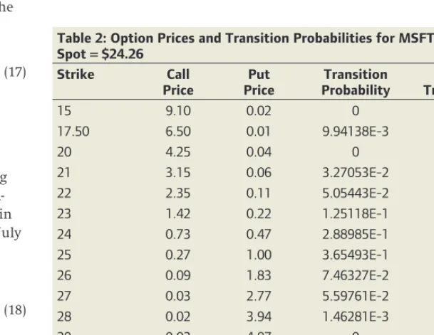
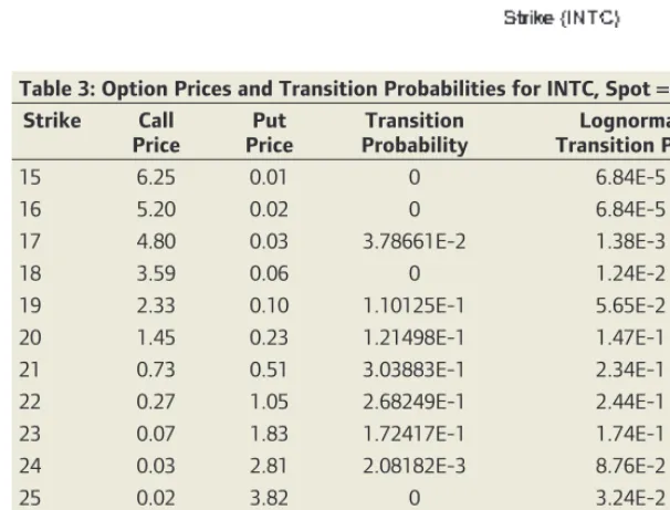
Option prices for the next expiration period were used to calculate the transition probabilities1. Probabilities extracted from call and put prices were used above and below the current price of the underlying stock. The transition probabilities for MSFT and INTC have been plotted and tabulated. When compared against Gaussian distribution, excess kurtosis can be seen in fatter tails.
Monte-Carlo simulation is performed with 10000 steps to get a 99% VaR. R language has been used to implement the Monte Carlo simulator. Random number generator from R package Tinflex (Leydold, Botts, and Hörmann, 2011) was used in the Monte Carlo simulation2. VaR from 10 Monte Carlo simulation runs is shown in table 4. VaR obtained is compared against that from delta-normal method. The Value-at-Risk obtained from Monte-Carlo simulation ($93303.3) is higher than that obtained from delta-normal method ($87870.90). This reflects a greater tail risk in returns as implied from option prices.
The difference in VaR calculated using this method (Monte-Carlo simula-tion) and delta-normal method becomes more pronounced as the difference in historical volatility and the expected volatility in the future (as reflected in option prices) becomes larger. Another sample run for calculating the
General Electric (GE) 5000 $18.49
Total $510400
Table 2: Option Prices and Transition Probabilities for MSFT, Spot = $24.26
15 9.10 0.02 0 4.57E-10
17.50 6.50 0.01 9.94138E-3 4.57E-10
20 4.25 0.04 0 3.42E-4
21 3.15 0.06 3.27053E-2 3.32E-3
22 2.35 0.11 5.05443E-2 3.11E-2
23 1.42 0.22 1.25118E-1 1.27E-1
24 0.73 0.47 2.88985E-1 2.61E-1
25 0.27 1.00 3.65493E-1 2.93E-1
26 0.09 1.83 7.46327E-2 1.90E-1
27 0.03 2.77 5.59761E-2 7.37E-2
28 0.02 3.94 1.46281E-3 1.76E-2
29 0.02 4.87 0 2.69E-3
30 0.02 6.20 5.84661E-3 2.72E-4
31 0.02 6.87 0 1.89E-5
32 0.01 7.80 2.03898E-2 9.43E-7
33 0.01 8.80 0 3.46E-8
56-61_Ahlawat_TP_May_2012_Final.58 58
TECHNICAL PAPER
^
Wilmott
magazine
59
^
Table 4: Monte-Carlo Simulation Results for 99% VaR using 10000 Steps
Run 99% VaR
1 $92685.5
2 $94428.4
3 $95590.3
4 $96552.7
5 $92994.3
6 $93103.3
7 $94514.7
8 $93083.7
9 $94245.9
10 $93303.3
Average $93933.99
Standard Deviation 1231.19
Table 3: Option Prices and Transition Probabilities for INTC, Spot = $21.20
Strike Call
Price
Put Price
Transition Probability
Lognormal Transition Prob
15 6.25 0.01 0 6.84E-5
16 5.20 0.02 0 6.84E-5
17 4.80 0.03 3.78661E-2 1.38E-3
18 3.59 0.06 0 1.24E-2
19 2.33 0.10 1.10125E-1 5.65E-2
20 1.45 0.23 1.21498E-1 1.47E-1
21 0.73 0.51 3.03883E-1 2.34E-1
22 0.27 1.05 2.68249E-1 2.44E-1
23 0.07 1.83 1.72417E-1 1.74E-1
24 0.03 2.81 2.08182E-3 8.76E-2
25 0.02 3.82 0 3.24E-2
26 0.01 4.50 8.96828E-4 9.06E-3
27 0.01 4.25 5.71573E-2 1.98E-3
28 0.04 – 0 3.45E-4
30 0.02 8.13 0 5.89E-6
Figure 1: Market Implied Transition Probability from Option Prices and Lognormal Transition Probability for MSFT (Spot = $24.26) and INTC (Spot = $21.20).
September 19, 2011 and closed at 19.99 on June 20, 2011, indicating a signifi-cantly higher market volatility for the second run. One month VaR for the test portfolio calculated using option-implied probability distribution with Monte-Carlo method has a mean of $110868.50 and a standard deviation of 883.84 while the VaR calculated using delta-normal method using one month historical variance is $93986.40.
VaR of the test portfolio defined in table (1) was run for September 19, 2011. Taking VIX, CBOE Volatility Index for S&P 500 (CBOE Volatility Index®, 2009), as a measure of market volatility, we find that VIX closed at 32.73 on
56-61_Ahlawat_TP_May_2012_Final.59 59
60
Wilmott
magazine
Appendix: Supporting Calculation Results
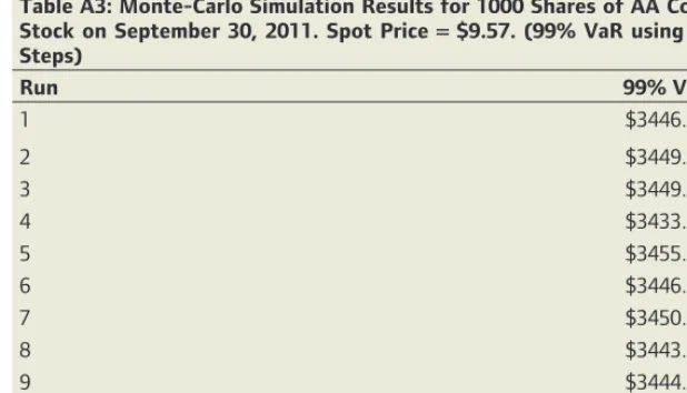
dates fall before the options expiry (October 21 2011). Simulations show that for a position comprising 1000 shares of Alcoa, the VaR using Monte-Carlo based simulation is $3446.58 (with standard deviation of 6.2312). VaR for this position using delta-normal method is higher at $4880.55. This is because options based probability distribution is implying a higher prob-ability of a positive earnings surprise, thereby reducing the downside risk. Similary, VaR for a position of 1000 shares of Intel (INTC) common stock has an average VaR of $6112.60 using monte-Carlo based simulation method, but is $10878 using delta-normal method. The detailed results are present-ed in Appendix.
In equation (20) and (21) σi denotes the standard deviation in daily log return for asset i. Ni(0, 1) is a random number drawn from standard nor-mal distribution (mean = 0 and variance = 1). W denotes a column vector composed of asset values (at time t = 0), Wi = NiSi(0). Σ denotes the covariance matrix of log returns.
(T)=
n
i=1 NiSi(T)
(T)−(0)
(0) =
NiS(0)
exp
−σ2 iT 2 +σi
√
TNi(0, 1) −1
NiS(0)
=Wi
exp
−σi2T
2 +σi
√
TNi(0, 1)
−1
≈Wi
−σ2
iT
2 +σi
√
TNi(0, 1)
=Wi−
σi2T
2 +N(0,W
W)
(20)
⇒VaR99%=(0)
−Wi
σ2
iT
2 −2.33
√
WW
=$87870.90 (21)
4 Data Source
Options data and historical price quotes (daily close price) were obtained from Yahoo Finance website http://finance.yahoo.com. Historical prices and option chains are freely available for each ticker on this website.
5 Conclusion
VaR based on market implied probability distribution is able to capture the effect of upcoming events. For example, just before quarterly earnings release the probability distribution increases for strikes above and below the spot price reflecting a greater probability of up or down jumps. Also, after sharp drops in asset price, the probability distribution shifts to the right echoing the option traders view of likely recovery in asset price. The method
ENDNOTES
1.The tridiagonal matrix from equation (8) was solved using R pack limSolve (Soetaert, Van den Meersche, and van Oevelen, 2009).
2. Tinflex package (Leydold, Botts, and Hörmann, 2011) allows random number generation from specified probablity distribution.
REFERENCES
Berkowitz, J., O’Brien., J. 2002. How Accurate Are Value-at-Risk Models at Commercial Banks? Journal of Finance 57(3).
Bohdalová, M. 2007. A Comparison of Value-at-Risk Methods for Measurement of the Financial Risk. E-Leader conference, Prague. http://www.g-casa.com, ISSN: 1935-4819. Bollerslev,T. 1986. Generalized Autoregressive Conditional Heteroskedasticity. Journal of Econometrics 31(3), 307–327.
Breeden, D. and Litzenberger, R. 1978. Prices of State Contingent Claims Implicit in Options Prices. Journal of Business 51(4), 621–651.
CBOE Volatility Index® (VIXR®). 2009. Chicago Board Options Exchange, Inc. http://www. cboe.com/micro/vix/vixwhite.pdf.
Derman, E. and Kani, I. 1994. The Volatility Smile and Its Implied Tree. Risk 7(2), 139–145.
Laubsch, A. 1999. Risk Management: A Practical Guide. RiskMetrics Group (MSCI): New York.
Leydold, J., Botts, C. and Hörmann, W. 2011. Tinflex:Tinflex-Universal non-uniform ran-dom number generator. Open source R-package version 0.1. http://CRAN.R-project.org /package=Tinflex.
Nelson, DB. 1991. Conditional Heteroskedasticity in Asset Returns: A New Approach.
Econometrica 59(2), 347–370.
Pritzker, M. 2001.The Hidden Dangers of Historical Simulation. Finance and Economics Discussion Series. Board of Governors of the Federal Reserve System: Washington, DC. Soetaert, K., Van den Meersche, K. and van Oevelen, D. 2009. limSolve: Solving Linear Inverse Models. R-package version1.5.1.
Zangari, P. 1996. Risk Metrics technical document. JP Morgan and Reuters: New York.
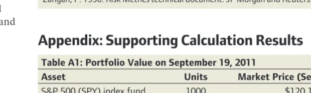
Table A1: Portfolio Value on September 19, 2011
Asset Units Market Price (Sept 19, 2011)
S&P 500 (SPY) index fund 1000 $120.17 Microsoft Corp (MSFT) 5000 $26.98
Intel Corp (INTC) 8000 $22.20
General Electric (GE) 5000 $16.04
Total $512870
assets that do not have traded options.
Samit Ahlawat is a Portfolio Manager at WorldQuant LLC, working on statistical arbitrage strategies in equities. He has worked as Vice President at Citigroup in credit derivatives and at Citadel Investment Group LLC. He completed his Masters degree from University of Illinois, Urbana Champaign specializing in numerical computation methods. He has an active interest in creating open source software for scientific computation.
56-61_Ahlawat_TP_May_2012_Final.60 60
TECHNICAL PAPER
Wilmott
magazine
61
W
Table A3: Monte-Carlo Simulation Results for 1000 Shares of AA Common Stock on September 30, 2011. Spot Price = $9.57. (99% VaR using 10000 Steps)
Run 99% VaR
1 $3446.33
2 $3449.04
3 $3449.81
4 $3433.19
5 $3455.59
6 $3446.33
7 $3450.96
8 $3443.24
9 $3444.79
10 $3446.57
Average $3446.59
Standard Deviation 6.23
Table A4: Monte-Carlo Simulation Results for 1000 Shares of INTC Common Stock on September 30, 2011. Spot Price = $21.33. (99% VaR using 10000 Steps)
Run 99% VaR
1 $6117.86
2 $6123.85
3 $6093.23
4 $6129.17
5 $6117.86
6 $6068.56
7 $6109.88
8 $6118.53
9 $6119.86
10 $6127.17
Average $6112.60
Standard Deviation 18.49
Table A2: Monte-Carlo Simulation Results for Test Portfolio on September 19, 2011. (99% VaR using 10000 Steps)
Run 99% VaR
1 $110332.00
2 $110116.00
3 $111191.00
4 $110749.00
5 $112535.00
6 $111880.00
7 $110146.00
8 $111401.00
9 $109683.00
10 $110652.00
Average $110868.50
Standard Deviation 883.84
56-61_Ahlawat_TP_May_2012_Final.61 61