Proceedings of the IJCNLP-08 Workshop on NLP for Less Privileged Languages, pages 105–112,
Abstract
Human computer interaction through Natural Language Conversational Interfaces plays a very important role in improving the usage of computers for the common man. It is the need of time to bring human computer interaction as close to human-human interaction as possible. There are two main challenges that are to be faced in implementing such an interface that enables interaction in a way similar to human-human interaction. These are Speech to Text conversion i.e. Speech Recognition & Text To Speech (TTS) conversion. In this paper the implementation of one issue Speech Recognition for Indian Languages is presented.
1 Introduction
In India if it could be possible to provide human like interaction with the machine, the common man will be able to get the benefits of information and communication technologies. In this scenario the acceptance and usability of the information technology by the masses will be tremendously increased. Moreover 70% of the Indian population lives in rural areas so it becomes even more important for them to have speech enabled computer application built in their native language.
Here we must mention that in the past time decades, the research has been done on continuous, large vocabulary speech processing systems for English and other European languages; Indian languages as Hindi and others were not being emphasized. For example for English language,
Implementing a Speech Recognition System Interface for Indian
Languages
the commercial speech recognition systems available in the market are IBM Via Voice and Scansoft Dragon system. These have mature ASR engines with high accuracy. No such system with this accuracy is available for Hindi (Kumar et al., 2004). India is passing through the phase of computer revolution. Therefore it is need of time that speech processing technology must be developed for Indian languages.
Fortunately people have realized the great need of human machine interaction based on Indian languages. Researchers are striving hard currently to improve the accuracy of the speech processing techniques in these languages (Samudravijaya, 2000). Speech technology has made great progress with the development of better acoustic models, new feature extraction algorithms, better Natural Language Processing (NLP) and Digital Signal Processing (DSP) tools and significantly better hardware and software resources.
Through this paper, we describe the development of ASR system for Indian languages. The challenges involved in the development are met by preparing various algorithms and executing these algorithms using a high level language VC++. Currently a Speech-In, Text-Out interface is implemented.
The paper is organized as follows: section 2 presents the architecture and functioning of ASR. Section 3 describes the modeling and design used for speech recognition system. Section 4 describes the experiments & results. Section 5 describes the conclusion and future work.
2 Architecture of ASR
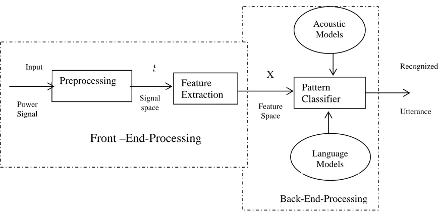
The basic structure of a speech recognition system
R. K. Aggarwal
Mayank Dave
Deptt. Of Computer Engg.
Deptt. Of Computer Engg.
N.I.T. Kurukshetra
N.I.T. Kurukshetra
[email protected]
[email protected]
is shown in figure 1.
2.1 Preprocessing
It covers mainly these tasks- A/D conversion, Background noise filtering, Pre emphasis, Blocking and Windowing.
In first task analog electrical signals are digitized, i.e. these are converted into a discrete-time, discrete-valued signal. This process of analog to digital conversion has two steps: sampling and quantization.A signal is sampled by measuring its amplitude at a particular time; the sampling rate is the number of samples taken per second. In general, a sampling rate between 8 and 20 kHz is used for speech recognition application (James Allen, 2005). As a point of reference, perceptual studies generally indicate that frequencies up to about 10 kHz (10,000 cycles per second) occur in speech, but speech remains intelligible within a considerably narrower range.
The second important factor is the quantization factor, which determines what scale is used to represent the signal intensity. Generally, it appears that 11-bit numbers capture sufficient information, although by using a log scale, we can get by with 8-bit numbers. In fact, most current speech recognition systems end up classifying each segment of signal into only one of 256 distinct categories.
Acoustic Models
So a typical representation of a speech signal is a stream of 8-bit numbers at the rate of 10,000 numbers per second clearly a large amount of data. The challenge for speech recognition system is to reduce this data to some manageable representation.
Once signal conversion is complete, background noise is filtered to keep SNR high. While speech capturing, background noise and silence (absence of speech) will also be quantized with speech data. An important problem in speech processing is to detect the presence of speech in a background of noise and silence from our recording speech. This problem is often referred to as the endpoint detection problem (Rabiner and Bishnu, 1976). By accurately detecting the beginning and end of an utterance the amount of processing can be kept at minimum. According to literature (Reddy, 1976), accurate determination of end points is not very difficult if the signal-to-noise ratio is high, say greater than 60 dB.
The next step is the pre-emphasis. The motivation behind it is to emphasize the important frequency components in the signal (i.e. amplify important areas of the spectrum) by spectrally flatten the signal. For example hearing is more sensitive in the 1 KHz-5 KHz region of the spectrum. It amplifies this area of spectrum, assisting the spectral analysis algorithm in modeling the most perceptually important aspects of the speech spectrum.
Input Recognized
Utterance Preprocessing
S
X Feature
Extraction Pattern Classifier Signal
space Power
Signal Feature Space
Front –End-Processing
Language Models
Back-End-Processing
2.2 Feature Extraction/Parametric Transform
The goal of feature extraction is to find a set of properties of an utterance that have acoustic correlations in the speech signal, that is parameters that can some how be computed or estimated through processing of the signal waveform. Such parameters are termed as features. Feature extraction is the parameterization of the speech signal. It includes the process of measuring some important characteristic of the signal such as energy or frequency response (i.e. signal measurement), augmenting these measurements with some perceptually meaningful derived measurements (i.e. signal parameterization), and statically conditioning these numbers to form observation vectors.
There are several ways to extract features from speech signal as given below:
• Linear Predictive Cepstral Coefficients (LPCC)
• Mel Frequency Cepstral Coefficients (MFCC) (Skowronski et al., 2002)
• Wavelet as feature extractor (Biem, 2001) • Missing feature approach (Raj et al., 2005)
2.3 Acoustic Modeling
In this subsystem, the connection between the acoustic information and phonetics is established. Speech unit is mapped to its acoustic counterpart using temporal models as speech is a temporal signal. There are many models for this purpose like,
• Hidden Markov Model (HMM)
• Artificial Neural Network (Rao et al.,2004)
• Dynamic Bayesian Network (DBN) (Huo et al., 1997)
ANN is a general pattern recognition model which found its use in ASR in the early years. Rabiner (1991), first suggested the HMM approach leading to substantial performance improvement. Current major ASR systems use HMM for acoustic modeling. Since then researchers have tried to optimize this model for memory and computation requirements. In the current state, it seems that
HMM has given the best it could and now we need to find other models to go ahead in this domain. This leads to consideration of other models in which Dynamic Bayesian Network seems a promising direction
Still our experiments and verification has been done on a HMM based system.
2.4 Language Modeling
The goal of language modeling is to produce accurate value of probability of a word W, Pr(w). A language model contains the structural constraints available in the language to generate the probabilities. Intuitively speaking, it determines the probability of a word occurring after a word sequence. It is easy to see that each language has its own constraints for validity. The method and complexity of modeling language would vary with the speech application. This leads to mainly two approaches for language modeling. Generally, small vocabulary constrained tasks like phone dialing can be modeled by grammar based approach where as large applications like broadcast news transcription require stochastic approach.
3 Modeling and Design for Implementation
3.1 Signal Modeling and Front End Design
events in the probability space is called Signal Modeling (Picone, 1993; Karanjanadecha and Zoharian, 1999).
Signal Modeling can be divided into two basic steps: Preprocessing and Feature Extraction. Preprocessing is to pre-process the digital samples to make available them for feature extraction and recognition purpose. The steps followed during signal modeling are as following:
• Background Noise and Silence Removing • Pre emphasis
• Blocking into Frames • Windowing
• Autocorrelation Analysis • LPC Analysis
• LPC Parameter Conversion to Cepstral Coefficients
3.2 Back End Processing
The last section showed how the speech input can be passed through signal processing transformations and turned into a series of vectors of features, each vector representing one time slice of the input signal. How are these feature vectors turned into probabilities?
3.2.1 Computing Acoustic Probabilities
There are two popular versions of continuous approach. The more widespread of the two is the use of Gaussian pdfs, in the simplest version of
Word Model
Observation Sequence … …
(Special feature vectors)
which each state has a single Gaussian function which maps the observation vector Ot to a
probability. An alternative approach is the use of neural networks or multilayer preceptons which can also be trained to assign a probability to a real valued feature vector. HMMs with Gaussian observation-probability-estimators are trained by a simple extension to the forward-backward algorithm. HMMs with neural-net observation-probability-estimators are trained by a completely different algorithm known as error back-propagation.
3.2.2 HMM and its Significance to Speech Recognition:
Among the various acoustic models, HMM is so far the most widely used and most effective approach. Its popularity is due to an efficient algorithm for training and recognition and its performance superiority over the other modeling structures.
An HMM is a statistical model for an ordered sequence of symbols, acting as a stochastic finite state machine which is assumed to be build up from a finite set of possible states, each of those states being associated with a specific probability distribution or probability density function. Each state of machine represents a phonetic event and a symbol is generated each time a transition is made from one state to the next.
a24
a11 a22
………
O
3O
4 b1(o2)Start
a
2m
3end
a33
b1(o1)
r
1b2(o3) b
a01 a12 a23
2(o5)
b3(o6)
O
6O
1O
2O
5There are three basic problems related to HMM: the evolution problem, the decoding problem and the learning problem. These problems are addressed by Forward Algorithm, Viterbi Algorithm and Baum-Welch Algorithm respectively. A detailed discussion of the same is available here (Rabiner, 1989).
HMM-based recognition algorithms are classified into two acoustic models, i.e., level model and word-level model. The phoneme-level HMM has been widely used in current speech recognition systems which permit large sized vocabularies. Whereas the word-level HMM has excellent performance at isolated word tasks and is capable of representing speech transitions between phonemes. However its application has remained a research-level and been constrained to small sized vocabularies because of extremely high computation cost which is proportional to the number of HMM models. Recognition performance in the word HMM is determined by the number of HMM states and dimensions of feature vectors. Although high numbers of the states and the dimensions are effective in improving recognition accuracy, the computation cost is proportional to these parameters (Yoshizawa et al., 2004). As conventional methods in high-speed computation of the output probability, Gaussian selection (Knill et al., 1996) and tree structured probability density function (Watanabe et al., 1994) are proposed in the phoneme-level HMM. These methods use the approximation to the output probability if exact probability values are not required. However in the word HMM, output probability values directly effects recognition accuracy and a straight forward calculation produces the most successful recognition results (Yoshizawa et al., 2004).
To see how it can be applied to ASR, we are using a whole-word isolated word recognizer. In our system there is a HMM Mi for each word I the
dictionary D. HMM Mi is trained with the speech
samples of word Wi using the Baum-Welch
Algorithm. This completes the training part of the ASR. At the time of testing the unknown observation sequence O is scored against each of the models using the forward algorithm and the word corresponding to the highest scoring model is given as a recognized word.
For example HMM pronunciation network for the word “Ram”, given in figure 2 shows the transition probabilities A, a sample observation sequence O and output probabilities B. HMMs used in speech recognition usually use self loops on the states to model variable phone durations; longer phones require more loops through the HMM.
3.2.3 Language Modeling
In speech recognition the Language Model is used for speech segmentation. The task of finding word boundaries is called segmentation (Martin and Jurafsky, 2000). For example decode the following sentence.
[ ay hh er d s sh m th ih ng ax b aw m wh v ih ng r ih s en l ih ]
I heard something about moving recently. [ aa n iy dh ax] I need the.
4. Experiment & Results
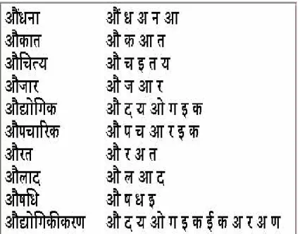
supports more than one pronunciation for a single word. There are various implementations of a dictionary; some load the entire dictionary on initialization whereas other implementations obtain pronunciation on demand. Thus dictionary is a file which provides a mapping from grapheme to phoneme for a given word. An example is shown in Table 1.
Table 1. An Example Dictionary
For recording, training and testing purpose we have designed a common interface as given in Figure 3.
Snapshot
Figure 3: Interface for ASR Functioning
First we decide the words on which experiment is to be performed and then write these words into the dictionary. After completing the transcript preparation and dictionary making step we are ready for the recording of our transcript. To record speech samples we click the record button of the
interface. Each word is recorded by specifying a different name. After recording all words the train button is pressed which does the statistical modeling. After this, to recognize the word, we press the speak button and say the word whichever we want to recognize. Note that the word to be recognized must be available in the dictionary.
When a word is recorded it tells us the number of frames (starting frame index, end frame index, number of frames used) by which word length has been covered.
After training, testing is performed. During testing it will count the right word match and display the accuracy after each word match.
We have tested the system for various parameters and get the following results.
4.1 Experiments with Different Number of Trainings
Two hundred isolated words of Hindi language are recorded and trained various numbers of times. Testing of randomly chosen fifty words is made and the results are as given in figure 4.
Figure 4: Accuracy vs. No. of Training
4.2 Experiment with Different Vocabulary Sizes
This fact is supported by results as shown in the graph of figure 5. System is trained five times and testing of randomly chosen twenty five words is made.
Figure 5. Accuracy vs. Words
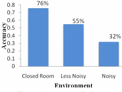
4.3 Experiments with Different Noise Environments
Experiment is performed in various noise environments: in closed room environment where noise energy is up to 7dB, in less noisy environment where noise energy vary 7dB to 12dB, in noisy environment where noise energy is above 12dB.
Figure 6. Accuracy vs. Environment
4.4 Experiments with Different Windows
To evaluate the effect of different windows such as Rectangular window, Hamming window, Hanning
Used Accuracy
Hamming window 76 %
ur
plement an SR for Indian language using LPCC for feature
as from limited
uous Speech
bruary 2001. Discriminative feature xtraction applied to speech recognition In IEEE window used in recognition of isolated Hindi words, a system of hundred isolated word is made. System is trained five times for each window. Twenty five results are made for each window using Hidden Markov Model for recognition. Dictionary size is of 100 words. Results obtained are given as
Window
Hanning window 69 % Rectangular window 55 %
5. Conclusion and Fut
e Work
We have proposed an approach to im A
extraction and HMM to generate speech acoustic model. Using our approach we have made a prototype of the recognizer for isolated word, speaker dependent ASR system for Hindi. The design of our system is such that it can be used to generate acoustic model for any Indian language and in a very easy way. The use of such an ASR solves the problem of technology acceptance in India by bringing human-human interaction closer to human-human interaction.
Scope for future work would concentrate on incorporating the features
vocabulary to large, from isolated word to connected words or continuous speech, from speaker dependent to speaker independent. We have tested our system for Hindi, it can be tested for other similar Indian languages like Sanskrit, Punjabi etc. with few modifications.
Even in European languages state of the art LVCSR (Large Vocabulary Contin
Recognition) systems are very far from the 100% accuracy. So people are trying new approaches apart from regular LPCC or MFCC at the front end and HMM as acoustic model at the back end. Wavelet and Dynamic Bayesian Network are two promising approaches that can be used for LVCSR systems in Indian languages.
References
. Missing-Feature
pproaches in Speech recognition. Signal
dy. 1976. Speech Recognition by achine: A Review, IEEE 64(4): 502-531.
atural anguage Understanding, Pearson Education.
h & anguage Processing, Pearson Education.
odeling echniques in Speech Recognition. IEEE Proc..
of aussian selection in large vocabulary continuous
. Computer Recognition of
poken Hindi. Proceeding of International
004. odelling Syllable Duration in Indian Languages
on Hidden arkov Models and Selected Applications in
Review of Neural etworks for Speech Recognition, Massachusetts
and J.G.Harris. 2002. reased MFCC Filter Bandwidth For
Noise-. Kumar, ANoise-. Verma & NNoise-.RajputNoise-. 2004Noise-. A Large
. Karanjanadecha and Stephan A. Zahorian.
. Huo, H. Jiang, & C.H. Lee. 1997. A Bayesian
awrence R. Rabiner and S. Atal Bishnu. 1976. A
wa, N. Wada, N. Hayasaka, and Y.
. Watanabe, K. Shinoda, K. Takagi, and E. Transactions on Acoustics, Speech, and Signal
Processing, vol. 9, pp. 96-108.
B. Raj and Stern. 2005 a
Processing magazine, IEEE Volume 22, Issue 5, pp. 101-116.
D. Raj Red M
James Allen. Third Edition 2005. N L
J. H. Martin and Daniel Jurafsky. 2000. Speec L
Joseph W. Picone. Sep. 1993. Signal M T
K.M.Knill, M.J.Gales and J. Young, 1996. Use G
speech recognition using HMMs, Proc. IEEE
ICSLP96, pp 470-473,
K. Samudravijaya. 2000 S
Conference of Speech, Music and Allied Signal Processing, Triruvananthapuram, pages 8-13.
K.S. Rao, B. Yegnanarayana. May 2 M
Using Neural Networks. In proceeding of ICASSP Montreal, Qubic, Canada, pp 313-316.
Lawrence R. Rabiner. 1989. A Tutorial M
Speech recognition, IEEE.
Lippman and P. Richard, N
Institutes of Technology (MIT) Lincoln Laboratory, U.S.A.
M. D. Skowronski Inc
Robust Phoneme Recognition. IEEE.
M
vocabulary Continuous Speech Recognition System for Hindi. In IBM Research Lab, vol.48 pp.703- 715 .
M
1999. Signal Modeling for Isolated Word Recognition, ICAS SP Vol 1, , p 293-296.
Q
predictive classification approach to robust speech recognition, in proc. IEEE ICASSP, pp.1547-1550.
L
Pattern Recognition Approach to Voice-Unvoiced-Silence Classification with Applications to Speech Recognition”, IEEE Transaction ASSP-24(3).
S. Yoshiza
Miyanaga. 2004.Scalable Architecture for Word
HMM-based Speech Recognition, Proc. IEEE
ISCAS .
T
Yamada, 1994. Speech recognition using tree-structured probability density function, Proc. IEEE ICSLP, pp 223-226.