Earthquake Moment Area Scaling Relations and the Effect of Fault Heterogeneity on Slow to Fast Earthquake Slip

(1)

and the Effect of Fault Heterogeneity on Slow to Fast

Earthquake Slip

Thesis by

Yingdi Luo

In Partial Fulfillment of the Requirements for the degree of

Doctor of Philosophy

CALIFORNIA INSTITUTE OF TECHNOLOGY Pasadena, California

2018

(2)

ORCID: 0000-0002-1165-6107

(3)

ACKNOWLEDGEMENTS

Pursuing a Ph.D. at Caltech has been the most wonderful journey and once-in-a-lifetime experience to me. For the past almost seven years, I have enjoyed beautiful sunshine of the Golden State, and the ultimate hospitality from local Californians. But most importantly, I enjoyed working with many many amazing and most tal-ented researchers and fellows at Caltech, who have accompanied me and shaped me in so many ways.

First and foremost, I would like to thank Pablo Ampuero, who is not only my Ph.D. advisor, but more the mentor of my life. Pablo has a sharp mind, keen ob-servation, and is always full of energy and curiosity. Working together we have brainstormed so many amazing ideas, although most of them are just gone with the wind because of my laziness and dumbness. Nevertheless, Pablo has always been absolutely supportive and patient on my slow progress and sloppiness from time to time. Thank you for being so awesome!

I would also like to thank Don Helmberger. Being my co-advisor in my first year, Don has again and again stunned me with his enigmatically sophisticated knowledge in seismology: having a peek on a seismogram, pointing to some arrival phases and telling me ’Hey I bet there’s some rough structure near the interface’ sounded like magic to me, but Don proved it to be solid science. Don is simultaneously serious and humorous. Thank you for being so amazing!

I would like to thank my former academic advisor Victor Tsai and Jennifer Jack-son, who helped me a lot caring for my academic progress and giving useful advices.

I would also like to thank the rest of my thesis committee members: Rob Clay-ton, Jean-Philippe Avouac and Nadia Lapusta, for dedicating your precious time to reading my thesis and tracking its progress.

(4)

discussion together), Mark Simons (being on my TAC committee, unfortunately absent from my Thesis committee due to time conflicts), Hiroo Kanamori, Tom Heaton, Joann Stock, Mike Gurnis, Paul Asimow and Joe Kirschvink.

I would as well thank all my colleagues that I worked with and helped me in various ways: Paul Somerville at AECOM, Anatoly Petukhin at GRI, Heidi Hous-ton at U. WashingHous-ton, Bruce Shaw at Lamont, Allan Rubin at PrinceHous-ton, Zhen Liu at JPL, Risheng Chu and Sidao Ni at China Academy of Science, Yoshi Kaneko at GNS, NZ, Sylvain Barbot at NTU, SG.

I thank Xiaofei Chen, my undergraduate advisor, who opened the door for me to the amazing world of Geophysics and recommended me over to Caltech, the best place to study Geophysics.

I would also like to say thank you to all the current and former Seismo Lab and GPS staff, especially Donna, Priscilla, Julia, Kim, Julie, Dian, Viola, Rosemary and Naveed. I thank you all for your dedicated work. I really enjoyed chatting with all of you.

Thank you to my best buddies here, Junle (buddy home-towner), Lingsen (gym partner and gaming buddy), Zhan (buddy USTCer and a good cook), Dongzhou (amazing Wiki contributor), Yiran and Dunzhu (Seismolab cohort and lovely cou-ple), Yihe (great event organizer), Kangchen (genius computer geek), Xiaolin (in the lab every weekend). I really enjoy hanging out with you, guys.

I thank all the other current and former members of our research group: Jess, Asaf, Surendra, Zacharie, Olivier, Han, Benjamin, Bryan, Percy. It is a great plea-sure to work with you guys and I learned a lot.

I also want to thank all current and former officemates in SM368: Rachel (unlimited cookie supply!), Chris, Ethan, Celeste, Natalia, Albert, Michelle, Dan, Qingyang. You all made the office welcoming and vivid, especially all my current officemates, who must be tolerating a lot with my endless and endless typing on my ultra-clicky mechanical keyboard recently. Thank you for your understanding!

(5)

Zhong-wen, and occasionally Victor. I’m not a particularly good player, but I enjoy playing with you, guys.

I also thank other Seismo Lab and GPS fellows: Zhihong, Daoyuan, Bing, Xi-angyan, Ting, Wei, Yanghui, Voon, Semechah, Minyan, Zhe, Xi Zhang, Xuan, Brent, Miki, Lingling, Xi Liu, Men-Andrin, Junjie, Hao. You are all wonderful!

Thank you as well to other fellow students at Caltech: Linghu, Wendy, Liang, Jiang and Brian for being nice to me.

My gratitude also goes to Ta-liang, former Seismological Laboratory fellow and USC professor emeritus of Geophysics, and Evelyn, USC professor emeritus of Neurology, for taking care of me and treating me like their child. You are so nice!

I owe my special thanks to my fiancée Vera, for your love and understanding. Having 2500 miles apart is tough. Having a Ph.D. candidate boyfriend is tougher. Having a Ph.D. candidate boyfriend 2500 miles away who is dull and stupid is tanπ₂ tough. Yet we have overcome all kinds of strenuous terrains holding hands together. With you, my life is meaningful and colorful, and thus we journey on.

Last but not least, I thank my parents, Jianhua and Yunqing, for your uncondi-tional love and eternal support on whatever I do. I feel sorry for being so far away as the only child they have. My mom cried when I went to USTC, 300 miles away from home. Now I’m in the States, 6000 miles away. Thus I also thank my fel-low golden-retriever, "HuTou", ("Tiger-head" in Chinese), for taking my role and accompanying my parents.

I love you all.

(6)

ABSTRACT

Earthquake moment-area scaling relations play a key role in both earthquake physics studies and earthquake hazard assessment. A three-stage moment-area relation, based on advances in earthquake source inversion, is currently in use in Japan. The second stage has a scaling exponent outside the range of commonly accepted models of small and very large earthquakes. We develop theoretical insight on the mechanical origin of this second-stage scaling. We utilize an analytical disloca-tion model, a numerical crack model and multi-cycle rate-and-state simuladisloca-tions of strike-slip faults with heterogeneous friction properties. We find that the second stage in earthquake moment-area scaling results from a combination of surface rup-ture effects, comprising an effective ruprup-ture elongation along-dip due to a mirror effect and systematic changes of the shape factor relating slip to stress drop. Based on this physical insight, we propose a simplified formula to account for these effects in moment-area scaling relations.

(7)

(8)

PUBLISHED CONTENT AND CONTRIBUTIONS

Luo, Y., J. P. Ampuero, K. Miyakoshi, and K. Irikura, (2017).

"Surface Rupture Effects on Earthquake Moment-Area Scaling Relations." Pure and Applied Geophysics, 1-12, doi:10.1007/s00024-017-1467-4.

Luo and Ampuero co-designed study and analyzed theoretical models. Luo per-formed all the rate-and-sate simulations and analyzed the results; produced all figures and drafted the manuscript. Miyakoshi and Irikura inspired the study and contributed to contend of observations and addressing corresponding reviewers’ comments. Both Luo and Ampuero contributed to interpreting the results and real-world implications.

Y. Luo, J. P. Ampuero, P. Galvez, M. van den Ende and B. Idini (2017). "QDYN: a Quasi-DYNamic earthquake simulator (v1.1)"

Zenodo. doi:10.5281/zenodo.322459

Luo and Ampuero co-developed the numerical code. Luo developed most pre-processing and post-pre-processing packages and example packages; drafted the code manual. Galvez implemented MPI, van den Ende and Idini developed additional functionalities of the code and Python wrappers.

Y. Luo and J. P. Ampuero, (2017)

"Stability and effective friction of faults with heterogeneous friction properties and fluid pressure"

Submitted

(9)

INTRODUCTION

This dissertation on theoretical and computational earthquake modeling includes two parts.

Part I consists of Chapter 2 and is focused on the mechanical origin of earthquake moment-area scaling relations. It is based on material published in

Luo, Y., Ampuero, J. P., Miyakoshi, K., and Irikura, K. (2017). Surface Rupture Effects on Earthquake Moment-Area Scaling Relations.

Pure and Applied Geophysics, 1-12, doi:10.1007/s00024-017-1467-4. Topical Volume on "Best Practices in Physics-based Fault Rupture Models for

Seismic Hazard Assessment of Nuclear Installations"

In this chapter we explore the origin of an intriguing intermediate regime in a scaling relation between earthquake moment and rupture area currently in use for ground motion prediction in Japan, which has a scaling exponent outside the range of expo-nents predicted by commonly accepted models of small and very large earthquakes. This scaling regime for earthquakes of intermediate sizes, or “second stage”, is scarcely studied but critical for earthquake hazard assessment; ignoring it can lead to underestimation of the seismic moment that can be released by a fault of a certain size. To investigate the mechanical origin of the second stage, we utilize an ana-lytical dislocation model, a numerical crack model and multi-cycle rate-and-state simulations. The latter comprise heterogeneous strike-slip faults with stochastic spatial distributions of characteristic slip distance. We find that the second stage emerges from a combination of surface rupture effects, comprising an effective rupture elongation along-dip due to a mirror effect and systematic changes of the shape factor relating slip to stress drop. Based on this physical insight, we propose a simplified formula to account for these effects in moment-area scaling relations.

(11)

Chapter 3 we study a heterogeneous fault model with a regularly alternating mixture of competent and incompetent materials and spatial contrasts of fault zone pore fluid pressure. We find that fault behaviors transit from fast earthquakes to slow earth-quakes, and to completely stable (steady sliding), controlled by both the mixture composition (the proportion of brittle and ductile materials) as well as the relative strength between the two alternating materials (via difference in pore pressure). We then utilize an analytical method, Linear Stability Analysis, and find it predicts the overall fault stability very well. We further study the fault stability with heuristic ap-proximations based on physical insights, and propose simple criteria that accurately predict the stability of slip on a heterogeneous fault.

Based on this fundamental study, in Chapter 4 we develop a model of competent as-perities with stochastic properties embedded in a frictionally stable fault matrix. We find that, compared to the regularly alternating model, the model with stochastic het-erogeneity permits slow slip behavior over a much wider range of model parameters. The model reproduces the hierarchical tremor migration patterns and accompany-ing slow slip events in quantitative agreement with observations in the Cascadia subduction zone. The tremor activities observed in Cascadia feature distinct tremor propagation speeds in different directions, including Rapid Tremor Reversals (RTR, backward propagating tremor) with a propagating speed 5-50 times faster than the forward tremor migration. We compared two end-member models, which differ by the assumed rheology of the fault zone matrix: in one model slow slip drives tremor, in the other tremor drives slow slip. Comparing the two models with observations we find that, in contrast to a common view, slow slip is likely the result of tremor activity rather than the cause.

Part I and Part II are related by the use of rate-and-state models that incorporate fault heterogeneities. These are building blocks towards the ultimate goal to understand the mechanics underlying the broad range of fault slip behaviors observed in nature, from small to large, slow to fast.

(12)

C h a p t e r 2

SURFACE RUPTURE EFFECTS ON EARTHQUAKE

MOMENT-AREA SCALING RELATIONS

Abstract

Empirical earthquake scaling relations play a central role in fundamental studies of earthquake physics and in current practice of earthquake hazard assessment, and are being refined by advances in earthquake source analysis. A scaling relation between seismic moment (M₀) and rupture area (A) currently in use for ground motion prediction in Japan features a transition regime of the form M0 ∼ A2, between the well-recognized small (self-similar) and very large (W-model) earthquake regimes, which has counter-intuitive attributes and uncertain theoretical underpinnings. Here, we investigate the mechanical origin of this transition regime via earthquake cycle simulations, analytical dislocation models and numerical crack models on strike-slip faults. We find that, even if stress drop is assumed constant, the properties of the transition regime are controlled by surface rupture effects, comprising an effective rupture elongation along-dip due to a mirror effect and systematic changes of the shape factor relating slip to stress drop. Based on this physical insight, we propose a simplified formula to account for these effects in M0− A scaling relations for strike-slip earthquakes.

2.1 Introduction

Earthquake scaling relations are empirical relations between source parameters, such as seismic moment, rupture dimensions and average slip(e.g. Leonard 2010). They are significant in basic earthquake physics studies, as they constitute a first-order synthesis of static source properties to constrain earthquake mechanics models. They are also practically important as a key component of earthquake hazard assessment and ground motion prediction. Recent advances in observational techniques and source inversion methods are providing opportunities to refine the empirical relations between seismic moment and rupture geometry(Miyakoshi et al. 2015; Murotani et al. 2015)and to better understand their underlying physics.

Observations of strike-slip earthquakes show two end-member regimes in the scaling of seismic moment (M0) vs. rupture area (A): M0 ∼ A3

/₂

(13)

should be M0 ∼ A n

with an exponent ntaking intermediate values, 1 < n < 3/2. However, some authors have proposed values of n larger than 3/2. In particular, Irikura and Miyake (2011)introduced aM0vs. Ascaling relation with three scaling regimes (referred to hereafter as Stages 1, 2 and 3, in increasing order of M0) andn = 2 at intermediate magnitudes (see also(Fujii and Matsu’ura 2000; Hanks and Bakun 2002; Irikura and Miyake 2001; Matsu’ura and Sato 1997; Murotani

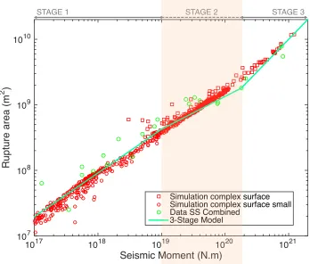
et al. 2015)). (Figure 2.1)shows the current version of the 3-stage scaling relation calibrated byMurotani et al. (2015). In contrast to previous studies that suffer from significant uncertainties on the rupture area (e.g. Wells and Coppersmith 1994), the work of Irikura and Miyake (2011) and follow up work are primarily based on rupture areas derived from kinematic source inversions(Miyakoshi et al. 2015; Murotani et al. 2015; Somerville et al. 1999; Song et al. 2008). While the empirical data strongly supports Stage 1, evidence for Stage 3 has been the subject of a long-standing debate due to the limited number of very large strike-slip earthquakes (Romanowicz and Rundle 1993; Scholz 1982). Hanks and Bakun (2002) and Irikura and Miyake (2001)independently proposed Stage 2,Murotani et al. (2015) calibrated its properties based on slip distributions inferred by source inversion, and Miyakoshi et al. (2015) analyzed a large amount of crustal earthquakes in Japan to confirm the existence of Stage 2. Our focus here on the 3-stage scaling relation introduced by Irikura and Miyake (2011)and calibrated byMurotani et al. (2015) is motivated by its wide adoption in ground motion prediction studies in Japan. The study of the 3-stage model, especially the least understood Stage 2, is of great importance in earthquake hazard estimation because the seismic moment predicted for a given rupture area, and hence strong ground motions, can be significantly higher if predictions include Stage 2.

(14)

Seismic Moment (N.m)

1017 1018 1019 1020 1021

Rupture area (m

2 )

107

108

109

1010

Simulation complex surface Simulation complex surface small Data SS Combined

3-Stage Model

STAGE 1 STAGE 2 STAGE 3

Figure 2.1: Earthquake seismic moment (M0) vs. rupture area (A) empirical and simulation data and 3-stage scaling model. Green curve: empirical 3-stage rela-tion by Murotani et al. (2015). Green circles: observational data from kinematic inversion of vertical strike-slip faults(Miyakoshi et al. 2015; Murotani et al. 2015; Somerville et al. 1999). Red circles and squares: synthetic earthquake data from our rate-and-state simulation of “reduced-scale” and “full-scale” models, respectively.

and Sato 1997), and scale-dependent stress drop(Dalguer et al. 2008). On the one hand, evidence for the deep rupture penetration required by Shaw’s model (up to 46 km depth inFigure 2.2) and for scale-dependent stress drop are scarce(e.g. Hanks and Bakun 2014). On the other hand, the model by (Matsu’ura and Sato 1997) assumes that the depth of the lithosphere and the depth of the seismogenic zone are the same, which is inconsistent with the current view that faults slip aseismically in the lower crust. Hence, the mechanical origin of Stage 2 remains unclear.

(15)

1017 1018 1019 1020 1021

Rupture area (m

2 )

107 108 109 1010

Shaw ξ=2.3

Dislocation Model ξ=1 Dislocation Model ξ=0.5

3-Stage Model

STAGE 1 STAGE 2 STAGE 3

Figure 2.2: Earthquake M0 - A relations for dislocation and deep rupture penetration models. Brown curve: deep penetration model(Shaw 2009; Shaw and Wesnousky 2008). Dark blue curve: our dislocation model with free surface (Model D2,ξ = 1). Light blue curve: our dislocation model without free surface (Model D1,ξ = 0.5). Green curve: empirical 3-Stage relation by Murotani et al. (2015). Model D2 has Stage 2 while model D1 does not, which indicates that the free surface is key to Stage 2.

present results of rate-and-state earthquake cycle simulations with a wide magnitude range that are consistent with the observational data and the 3-stage scaling relation. In Section 2.3 we investigate dislocation models and find a geometrical effect of the free surface that contributes to Stage 2. In Section 2.4 we develop crack models that fit the proposed 3-stage model and reveal a shape factor effect of the free surface that further contributes to Stage 2. Based on our numerical and analytical results, we propose a simplified equation that captures the 3-stage earthquake scaling relation. 2.2 A rate-and-state earthquake cycle model

(16)

(17)

with minimum and averageLcof 2.7 km and 6 km, respectively, at the middle depth of the seismogenic zone. A "reduced-scale" set targets Stages 1 and 2 on smaller faults (64 km length) with half smallerDcand finer mesh. The nucleation size also varies between models with differentDcranges. The range of magnitudes obtained from these two sets of simulations have significant overlap, which allows us to verify that our composite approach does not generate artifacts in the scaling relations. The seismic events detected in all these simulations are combined in a single catalog with over 10,000 events whose seismic moments span over four orders-of-magnitude.

Figure 2.3: Rate-and-state model settings. Left: effective normal stress (blue curve) anda/bratio (red curve) as a function of depth. The seismogenic zone (a/b < 1) extends roughly from 2 to 20 km depth. Right: an example of heterogeneous distribution of characteristic slip distance Dcwith correlation length of 1 km.

We detect seismic events based on slip-rate thresholds. Because of significant slip rate fluctuations caused by the strong heterogeneity of Dc, the event detection pro-cedure artificially divides some large events into several smaller successive events. We crudely mitigate this unrealistic feature by treating events that occur less than 10 minutes apart as being part of the same rupture. This correction comes with the cost of possibly overlooking some very early aftershocks. However, manual inspection shows that the number of overlooked aftershocks is very limited, and our focus here is on earthquake scaling rather than individual events, hence the benefits of amendment greatly outweigh its limitations.

(18)

STAGE 1 STAGE 2 STAGE 3

(a) Dislocation Model (square-rectangular) _{free surface}

Seismogenic zone

(b) Crack Model (circular-elongated) _{free surface}

Seismogenic zone

Figure 2.4: Rupture geometry in different models considered in this study. (a) Dislocation model with square to rectangular rupture transition. (b) Crack model with circular to elongated rupture transition. (c) Rate-and-state model with self-similar to elongated rupture transition. The free surface mirror image effect applies to all models. The "attractor effect" (coalescence between real and mirror image ruptures) enhances Stage 2 in the rate-and-state model.

(19)

stress drop, ∆τr e f, and the scattering in the M0 − A scaling plots is significantly reduced. While earthquake moment-area data can be alternatively interpreted as resulting from scale-dependency of stress drop(Dalguer et al. 2008), validation of this hypothesis has been challenging due to the large uncertainties of seismological estimates of stress drops. Here we will demonstrate that a model with constant stress drop is sufficient to explain the main characteristics of Stage 2.

STAGE 1 STAGE 2 STAGE 3

Figure 2.5: Stress drop as a function of seismic moment from rate-and-state sim-ulations. Red circles and squares: synthetic earthquake data from rate-and-state simulation of “reduced-scale” and “full-scale” models, respectively. In stages 2 and 3 the variability of stress drop is small.

(20)

We then rescale the stress drop: we multiplyM0by∆τ/∆τr e f, where the stress drop

∆τ_{is tuned to obtain the best overall match to the empirical model. The moment and}

rupture area data from our simulation catalog after these post-processing steps are shown inFigure 2.1. The resultingM0−Ascaling is in reasonable agreement with the 3-stage empirical relation. The events transit from small, self-similar ruptures to large, elongated ruptures(Figure 2.4(c)), and theM0−Ascaling displays all the 3 stages. The best fitting model parameters have reasonable values: Ws = 20 km and

∆τ_{= 2.4 MPa. The best fitting seismogenic depth of our rate-and-state model is in}

the upper end of the typical range of seismogenic depths of real strike-slip faults. Penetration of rupture into the deep VS region is observed in the large events of our rate-and-state simulations (Stage 3), but remains modest, up to 2 km into the VS region (approximately 10% of seismogenic depth).

An additional set of simulations reveals the importance of the free surface in gener-ating Stage 2. We ran earthquake cycle simulations on a pure velocity-weakening, deeply buried fault. Other settings are comparable to those of the simulations intro-duced above; the main difference is the absence of the free surface in the new set. The resulting catalog shows Stages 1 and 3, but no Stage 2(Figure 2.6). In the next sections we develop a theoretical understanding of surface rupture effects onM0−A scaling relations.

2.3 Dislocation models

We first develop a dislocation model for which we can obtain an analytical expression of theM0−Arelation in closed form, allowing fundamental insight into the problem. Dislocation models are rupture models with prescribed uniform slip and rupture geometry. The rupture shapes are assumed square for small events with rupture length L < Ws and rectangular for large events with L > Ws (Figure 2.4(a)). We consider two cases: (D1) without free surface and (D2) with free surface. The latter is achieved by mirroring the rupture with respect to the free surface.

From formulas for the stress changes induced by a rectangular dislocation in un-bounded media(Gallovič 2008), we derive the following relation between average slip ¯dand stress drop∆τat the center of a dislocation of length L and widthW:

(21)

1017 1018 1019 1020 1021

Rupture area (m

2 )

107

108

109

1010

VW Buried VW Buried small VW Surface VW Surface small 3-Stage Model

STAGE 1 STAGE 2 STAGE 3

Figure 2.6: Effect of free surface on M0− Ascaling. Red circles and squares: syn-thetic earthquake data from rate-and-state simulation with free surface in “reduced-scale” and “full-“reduced-scale” models, respectively. blue circles and squares: synthetic earthquake data from rate-and-state simulation without free surface in “reduced-scale” and “full-“reduced-scale” models, respectively. Green curve: empirical 3-Stage rela-tion. The difference between the two rate-and-state models indicates that the free surface is key to Stage 2.

where

f(x, ν)= x 2+

1 x2+₁/(₁−ν)

ν is Poisson’s ratio and ξ is a dimensionless parameter accounting for the free surface: ξ = 0.5 for a deeply buried dislocation (D1) and ξ = 1 for a vertical strike-slip dislocation breaking the free surface (D2). The seismic moment is

M₀=G Ad¯ (2.2)

(22)

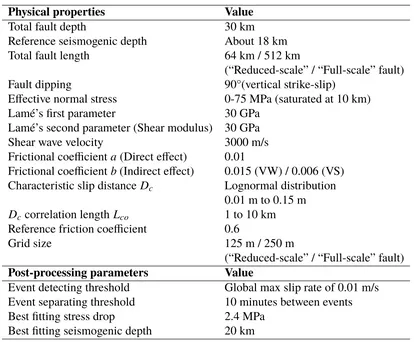
Physical properties Value

Total fault depth 30 km

Reference seismogenic depth About 18 km

Total fault length 64 km / 512 km

(“Reduced-scale” / “Full-scale” fault)

Fault dipping 90°(vertical strike-slip)

Effective normal stress 0-75 MPa (saturated at 10 km)

Lamé’s first parameter 30 GPa

Lamé’s second parameter (Shear modulus) 30 GPa

Shear wave velocity 3000 m/s

Frictional coefficienta(Direct effect) 0.01

Frictional coefficientb(Indirect effect) 0.015 (VW) / 0.006 (VS) Characteristic slip distanceDc Lognormal distribution

0.01 m to 0.15 m

Event detecting threshold Global max slip rate of 0.01 m/s Event separating threshold 10 minutes between events Best fitting stress drop 2.4 MPa

Best fitting seismogenic depth 20 km

Table 2.1: Typical parametric settings of rate-and-state simulation.

seismogenic depth, L > W =Ws and A= LWs. Combining Equations 2.1 and 2.2

(23)

M₀= A3/2_· π∆τ

Equation 2.4a shows that the dislocation model reproduces the M0 ∼ A3 /₂

scaling of Stage 1 whenL < Ws. By considering the asymptotic behavior of Equation 2.4b we find that the dislocation model also reproduces the M0 ∼ Ascaling of Stage 3 when L Ws. The resulting M0− Acurves, shown inFigure 2.2 (assumingWs = 20 km, ∆τ = 3 MPa for model D1 and ∆τ = 1.5 MPa for model D2), confirm that both models have Stages 1 and 3. However, only model D2 has a noticeable Stage 2, which appears in textcolorblueFigure 2.2 as an intermediate regime with lower slope than Stages 1 and 3. This confirms our previous conclusion that the free surface is essential for Stage 2.

In model D2, because of our simplified use of the mirror image method, the stress drop is actually evaluated at the surface rather than at mid-rupture depth. Evaluating it a mid-depth yields a more complicated formula and aM0− Arelation in between models D1 and D2.

An asymptotic argument provides insight on the role of the free surface. By extrap-olating equation 2.4b towardsL W s(AWs2), essentially considering ruptures that are elongated in the vertical direction, yields:

M₀= A

(24)

Our rate-and state simulations reveal an additional "surface attraction effect" that enhances the G effect. The shallow VS zone discourages small events from breaking the surface. Ruptures that grow to a certain size (still smaller thanWs) penetrate the shallow VS barrier and may break the free surface. Considering the free surface as a mirror, the real and image ruptures are two interacting coplanar cracks. The stress increase beyond their tips enhances their propagation, they attract each other and coalesce. This attractor effect can extend the vertical elongation beyond aspect ratio of 2, thus further enhancing the "G effect"(Figure 2.4(c)).

The dislocation model D2 agrees qualitatively with our rate-and-state model(Figure 2.7). However, it cannot fit the empirical Stages 1 and 3 simultaneously: the width of Stage 2 is narrower than in the empirical model. This limitation of dislocation models motivates our next improvement of the theory.

2.4 Crack models

We now consider crack models, i.e. models in which stress drop is prescribed within a given rupture area. There is no simple analytical M0− Aexpression for a crack of general shape and including the free surface, so we compute it numerically. The spatial distributions of slip and stress drop, discretized over a fault grid, are related by a linear system of equations whose coefficients can be computed with formulas by (Okada 1992). We prescribe a rupture geometry and uniform stress drop (∆τ), and solve the system of equations to obtain the slip distribution. We then compute the average slip ¯dand the “geometrical shape factor”Cdefined by

C =∆τmin(L,Ws)/Gd¯ (2.6)

Cis a non-dimensional function of L/Ws. KnowingC we can calculateM0of any given event using

M₀= G Ad¯= ∆τ_min(L,Ws)A/C (2.7)

(25)

TheM0−Acurve resulting from the crack model is shown in gray inFigure 2.7. This model also reproduces the 3 stages. Overall, it fits better the empirical relation than our dislocation models: it can fit Stages 1 and 3 simultaneously and has a reasonable range of Stage 2. The crack model also agrees well with our rate-and-state model.

STAGE 1 STAGE 2 STAGE 3

Figure 2.7: Earthquake M0− A scaling in empirical data, synthetic catalogs and theoretical models. Green circles: strike-slip earthquake data. Green curve: em-pirical 3-stage relation. Red circles and squares: synthetic earthquake data from earthquake cycle simulations of "reduced-scale" and "full-scale" models, respec-tively. Dark blue curve: dislocation model with free surface (Model D1). gray curve: crack model. Black curve: proposed simple equation 2.8 with best fitting parametersp= 2.08 andλ= 1.93. The crack model fits the data better than the dis-location model, and the simple equation 2.8 fits both the simulation and observation data extremely well.

(26)

Anderson 1975), which differ by a factor of about 4. Equation 2.7 shows that the decrease ofC pushes Stage 3 "to the right" in the M0− Aplot (larger moment for a given area). This effectively increases the apparent value of the scaling exponent n and extends the range of Stage 2. In nature, the C effect always occurs together with the G effect and both contribute to Stage 2. Thus the transition between small buried ruptures and large surface-breaking ruptures is the major origin of Stage 2. The combination of C effect and G effect, that we name "surface rupture effect", are sufficient to explain the observed Stage 2 in both real world earthquakes and simulated earthquakes.

Rupture Length / Ws

10-1 100 101

Shape factor C

0.5 1 1.5 2 2.5 3

2/π 7π/8

Shaw ξ=2.3

Dislocation Model ξ=1

Crack Model Simple EQ

Buried Surface-Breaking

Figure 2.8: Shape factor C of different models as a function of rupture length L normalized by seismogenic depth Ws. Brown curve: Shaw’s deep penetration model. blue curve: dislocation model with free surface (model D2). gray curve: crack model with free surface. Black curve: our proposed simple equation 2.8 with best fitting parameters p = 2.08 andλ = 1.93. The theoretical values of an infinitely long strike-slip rupture and a deep buried circular crack are 2/πand 7π/8, respectively.

(27)

a simplified equation in closed form for the shape factor C that can be useful for

This equation has the following controlling parameters: the seismogenic depthWs (or, in more general terms, the maximum rupture width) and two tunable variables pand λ. Similar to equations 2.4a,2.4b we get the following general forms of the M₀−Arelation

We performed a grid search to find the values of parameters pandλthat minimize the least squares misfit between the moment – area data from rate-and-state simula-tions (smoothed by a sliding median) and predicted by combining quasimula-tions 2.8 and 2.9a,2.9b. We find that the best fitting values and their 95% confidence intervals are p=2.08±0.2 andλ= 1.93±0.1(Figure 2.9).

Combining equations 2.8 and 2.9a,2.9b gives a convenient and reasonably accurate relation between seismic moments and rupture area across all earthquake magni-tudes. TheM0−Arelation resulting from equation 2.8 with the best fitting parameter valuespandλis presented in black inFigure 2.7. It is in very good agreement with both rate-and-state simulation results and the earthquake data and is noticeably bet-ter than the original crack model, especially in Stage 2. PlottingM0versus A/M

2/3 0 (Figure 2.10)allows a more critical assessment of the agreement between equation 2.8 and the synthetic rate-and-sate catalog.

(28)

it can be used as a simple yet accurate moment-area scaling model. Adopting the values p = 2 andλ= 2, within the 95% confidence level of the best fitting values, we propose the following simple equation for use in practical applications:

C

L Ws

= π

8

7− 3

1+(2Ws/L)2

(2.10)

Figure 2.9: Misfit between moment-area data from our rate-and-state catalog and our equation 2.8 as a function ofλandp. The best fitting values are p= 2.08 and λ=1.93 (light blue dot). White contours are the 95% and 99% confidence levels.

2.5 Conclusions

(29)

Seismic Moment: N.m

STAGE 1 STAGE 2 STAGE 3

Seismic Moment: N.m

STAGE 1 STAGE 2 STAGE 3

Figure 2.10: Left: earthquake M0− Ascaling in synthetic catalogs and best fitting simple practical model. Right: reduced M0−A/M

2/3

0 scaling, which allows a more critical assessment of the agreement between equation 2.8 and the synthetic rate-and-sate catalog. Gray circles: synthetic earthquake data from our rate-and-state simulation. Red curve: sliding median of synthetic data. Black curve: proposed simple equation 2.8 with best fitting parameters p = 2.08 and λ = 1.93. The proposed equation is in good agreement with the synthetic data.

layer and scale-dependency of stress drop, while possibly present and contribut-ing to the origin of the 3-stage model, should be considered as secondary. Based on this physical insight, we proposed a physically sound approximate formula that conveniently relates seismic moment and rupture size across all earthquake mag-nitudes, and can be of practical use in earthquake hazard assessment and ground motion prediction. The parameters of our rate-and-state model (seismogenic depth and stress drop) and of our simplified equation are calibrated to fit the empirical 3-stage model. While our models require a seismogenic depth of 20 km, in the upper end of typical values for strike-slip faults, including additional mechanisms like scale-dependency of stress drop might allow us to fit the real earthquake data with a smaller seismogenic depth.

(30)

References

Bodin, P. and J. N. Brune (1996), “On the scaling of slip with rupture length for shallow strike-slip earthquakes: Quasi-static models and dynamic rupture propagation”.Bulletin of the Seismological Society of America, 86 (5), pp. 1292– 1299.

Causse, M. and S. G. Song (2015), “Are stress drop and rupture velocity of earth-quakes independent? Insight from observed ground motion variability”. Geophys-ical Research Letters, 42 (18), pp. 7383–7389.

Dalguer, L. A., H. Miyake, S. M. Day, and K. Irikura (2008), “Surface rupturing and buried dynamic-rupture models calibrated with statistical observations of past earthquakes”.Bulletin of the Seismological Society of America, 98 (3), pp. 1147– 1161.

Fujii, Y. and M. Matsu’ura (2000), “Regional difference in scaling laws for large earthquakes and its tectonic implication”.Pure and Applied Geophysics, 157 (11), pp. 2283–2301.

Gallovič, F. (2008), “Heterogeneous Coulomb stress perturbation during earthquake cycles in a 3D rate-and-state fault model”.Geophysical Research Letters, 35 (21). Hanks, T. C. and W. H. Bakun (2002), “A bilinear source-scaling model for M-log A observations of continental earthquakes”.Bulletin of the Seismological Society of America, 92 (5), pp. 1841–1846.

– (2014), “M–logA Models and Other Curiosities”. Bulletin of the Seismological Society of America, 104 (5), pp. 2604–2610.

Hillers, G., Y. Ben-Zion, and P. M. Mai (2006), “Seismicity on a fault controlled by rate-and state-dependent friction with spatial variations of the critical slip distance”.Journal of Geophysical Research: Solid Earth, 111 (B1).

Hillers, G., P. M. Mai, Y. Ben-Zion, and J. P. Ampuero (2007), “Statistical properties of seismicity of fault zones at different evolutionary stages”.Geophysical Journal International, 169 (2), pp. 515–533.

Irikura, K. and H. Miyake (2001), “Prediction of strong ground motions for scenario earthquakes”.Journal of Geography (Chigaku Zasshi), 110 (6), pp. 849–875. – (2011), “Recipe for predicting strong ground motion from crustal earthquake

scenarios”.Pure and Applied Geophysics, 168 (1-2), pp. 85–104.

Kanamori, H. and D. L. Anderson (1975), “Theoretical basis of some empirical relations in seismology”.Bulletin of the seismological society of America, 65 (5), pp. 1073–1095.

(31)

Luo, Y., J. P. Ampuero, P. Galvez, M. Ende, and B. Idini (2017),QDYN: a Quasi-DYNamic earthquake simulator (v1.1). doi: 10.5281/zenodo.322459. url:

https://doi.org/10.5281/zenodo.322459_.

Mai, P. M. and G. C. Beroza (2000), “Source scaling properties from finite-fault-rupture models”.Bulletin of the Seismological Society of America, 90 (3), pp. 604– 615.

Marone, C. (1998), “Laboratory-derived friction laws and their application to seis-mic faulting”.Annual Review of Earth and Planetary Sciences, 26 (1), pp. 643– 696.

Matsu’ura, M. and T. Sato (1997), “Loading mechanism and scaling relations of large interplate earthquakes”.Tectonophysics, 277 (1), pp. 189–198.

Miyakoshi, K., K. Irikura, and K. Kamae (2015), “Re-examination of scaling rela-tionships of source parameters of the inland crustal earthquakes in Japan based on the waveform inversion of strong motion data”.Journal of Japan Association for Earthquake Engineering_{, 15 (7), pp. 141–156.}

Murotani, S., S. Matsushima, T. Azuma, K. Irikura, and S. Kitagawa (2015), “Scaling relations of source parameters of earthquakes occurring on inland crustal mega-fault systems”.Pure and Applied Geophysics, 172 (5), pp. 1371–1381.

Okada, Y. (1992), “Internal deformation due to shear and tensile faults in a half-space”.Bulletin of the Seismological Society of America, 82 (2), pp. 1018–1040. Romanowicz, B. and J. B. Rundle (1993), “On scaling relations for large earth-quakes”.Bulletin of the Seismological Society of America, 83 (4), pp. 1294–1297. Rubin, A. M. and J. P. Ampuero (2005), “Earthquake nucleation on (aging) rate and

state faults”.Journal of Geophysical Research: Solid Earth, 110 (B11).

Scholz, C. H. (1982), “Scaling laws for large earthquakes: consequences for physical models”.Bulletin of the Seismological Society of America, 72 (1), pp. 1–14. – (1998), “Earthquakes and friction laws”.Nature, 391 (6662), p. 37.

Shaw, B. E. (2009), “Constant stress drop from small to great earthquakes in magnitude-area scaling”.Bulletin of the Seismological Society of America, 99 (2A), pp. 871–875.

Shaw, B. E. and S. G. Wesnousky (2008), “Slip-length scaling in large earthquakes: The role of deep-penetrating slip below the seismogenic layer”. Bulletin of the Seismological Society of America, 98 (4), pp. 1633–1641.

Somerville, P. et al. (1999), “Characterizing crustal earthquake slip models for the prediction of strong ground motion”. Seismological Research Letters, 70 (1), pp. 59–80.

(32)

Streit, J. E. and S. F. Cox (2001), “Fluid pressures at hypocenters of moderate to large earthquakes”. Journal of Geophysical Research: Solid Earth, 106 (B2), pp. 2235–2243.

(33)

C h a p t e r 3

STABILITY AND EFFECTIVE FRICTION OF FAULTS WITH

HETEROGENEOUS FRICTION PROPERTIES AND FLUID

PRESSURE

Abstract

(34)

3.1 Introduction

Geological and physical background

The spectrum of earthquake phenomena has been greatly expanded by the discovery in the past decade of a family of slow earthquake processes including tectonic tremors (also known as non-volcanic tremors), low frequency earthquakes (LFE), very low frequency earthquakes (VLFE) and slow-slip events (SSE)(Ide et al. 2007). These seismic and aseismic events often occur together, for instance recurrent SSE are often accompanied by tremors, a phenomenon known in Cascadia as “episodic tremor and slow-slip events” (ETS). These slow earthquake phenomena mostly occur in the deep seismic-aseismic transition region of faults, or in the shallow accretionary prism of subduction zones. For instance, in the Cascadia subduction zone, ETS are located below the seismogenic depth limit determined by thermal modeling. In most cases, the transition from fast to slow, to stable slip behavior as a function of depth is gradual. With increasing depth, the inter-event time between episodic slow events (ETS and episodic tremors) and their duration decrease gradually. The amount of background (non-episodic, continuous) tremors increases with depth, and eventually transits into continuous steady slip(Wech and Creager 2011).

Regular earthquakes (i.e. earthquakes with rupture speed comparable to wave speeds) may also feature intermingled slow and fast rupture processes. Teleseismic back-projection source imaging of the 2011 Tohoku-Oki earthquake revealed a period of relatively slow rupture in the down-dip direction (Meng et al. 2011). This slow stage of the rupture was interspersed by strong high-frequency radiation bursts. The frequency content of this deeper part of the rupture, near the bottom of the seismogenic zone, was richer in high frequencies than the shallower part. This depth-dependent frequency content of the source has been observed in other megathrusts events, including the 2015 Gorkha, Nepal earthquake (Avouac et al. 2015; Lay et al. 2012).

These gradual transitions and coexistence of fast to slow earthquake slip behaviors in different environments suggest common mechanisms behind the full spectrum of earthquakes. Yet there is currently no model that can conceptually unify and quan-titatively reproduce such a large span of phenomena. This gap in our understanding of the mechanics of fast and slow earthquakes has encouraged us to search for viable physical models, and the present work is a building block in that effort.

(35)

block-in-matrix mélange, with competent lenses embedded in a incompetent block-in-matrix, at scales ranging from millimeters to tens of meters (Bebout and Barton 2002; Fagereng 2011; Fagereng and Cooper 2010; Fagereng and Sibson 2010; Meneghini et al.

2010). Laboratory experiments indicate that heterogeneity can affect the mechani-cal response of a fault. Kocharyan et al. (2016)found in laboratory experiments that the stress drop of slip transients depends on the proportion of materials mixed in a composite gouge. Ma and He (2001)found period doubling phenomena in experi-ments with two segexperi-ments of competent and incompetent materials along a frictional surface. Thus, fault heterogeneity involving contrasts of material competence is a potentially important ingredient to model rich fault slip behaviors.

Geological observations also show evidence of spatial and temporal variability of pore fluid pressure across various scales in fault zones. This contributes to fault heterogeneity and can affect the fault slip behavior. Mechanisms such as hydraulic fracturing and cracking(Luo and Vasseur 2002), and pore-space reduction by solution and cementation (Rittenhouse 1971) change the permeability of fault materials and affect the pore pressure and hence frictional strength. The formation of fluid seals in a fault zone causes high pore pressures if the sealed material compacts or produces more fluids. Excess pressure can then be released by rupture of the seals, over the long time scales of plate subduction, or recur with fault-valve behavior over the time periods between earthquakes(Hillers and Miller 2007; Sibson 1992, 2014; Sibson et al. 1988). Also, various direct and indirect evidences show localized changes in pore pressure. Healy et al. (1968)and a body of subsequent work studies seismicity changes due to changes of pore pressure. Thermal expansion of pore fluids, e.g. via shear heating, in media with heterogeneous permeability can create highly localized pore pressure contrasts (Osborne and Swarbrick 1997). Roberts and Nunn (1995)found that fluid transport results in localized pore pressure changes on various time scales. Fagereng and den Hartog (2017)studied pressure solution at seismogenic depths and found that more soluble elements dissolve first, which causes porosity and pore pressure differences between competent and incompetent fault materials at fine length scales of material heterogeneity.

(36)

and Kilgore (1993) found, in laboratory experiments, a scaling between Dc and the thickness of the gouge layer, a fault zone property that shows variability along natural faults. Scuderi and Collettini (2016) found thatDc is positively related to normal stress, which can also be variable along a fault. Parsons (2005)hypothesized that changes ofDccould help explain dynamic triggering.

Figure 3.1: Sketch of conceptual model, where asperities make solid-to-solid con-tact at fault surface and surrounded by a gouge matrix which can have different compressibility and permeability

(37)

3.1). Influx of fluids, e.g. due to dehydration, can change the pore pressure in the gouge but not in the sealed asperities. This results in differences of effective normal stress between asperities and the gouge matrix.

Background on fault stability

In theoretical and computational models, a fault can display a wide range of slip behaviors. We refer to a fault as "stable" if it slips steadily when driven by a steady loading. If instead the fault generates spontaneous slip transients, we qualify it as "unstable". On unstable faults, slip transients range from quasi-static (aseismic, such as SSE) to dynamic (seismic, such as regular earthquakes). The distinction between aseismic and seismic slip transients is based on radiation efficiency, i.e. the ratio of radiated energy to the sum of radiated and fracture energies. The radiation efficiency of an earthquake or any propagating slip transient is primarily controlled by its rupture speed (Venkataraman and Kanamori 2004). The stability of a fault depends on its frictional properties, state of stress and boundary conditions, as will be explained in detail in section 3.2 within the framework of rate-and-state friction. The propensity to stability of a rate-and-state material depends strongly on whether its steady-state friction coefficient is weakening (VW) or velocity-strengthening (VS). A VW material can be unstable and will represent here a competent fault zone material, whereas a VS material tends to be stable.

(38)

see also section 3.2). Yabe and Ide (2017)argued that the P-instability occurs when the size of the VW segment exceeds the critical size for instability on a homogeneous VW fault. We will show in section 3.2 that such argument, while adequate to first-order, is incomplete: the P-instability is affected by the surrounding VS material as well. They also found that, if the loading stiffness is very low, the T-instability occurs only if the fault is velocity neutral on average (average a − b = 0). This condition can be derived as a special case of the theoretical results bySkarbek et al. (2012). Viesca (2016)further studied the evolution of slip rate during the nucleation of frictional instabilities on heterogeneous faults.

Goals and scope

In this study, we focus on the following two questions about faults with mixture of competent/incompetent materials and pore pressure contrasts, within the framework of rate-and-state faults with alternating VS and VW properties:

1. Under what conditions is the fault stable or unstable? 2. Does unstable slip span the whole fault or only part of it?

In particular, our study includes an investigation on the effect of heterogeneous characteristic slip distance Dc, fault widthW, and effective normal stress contrast between the VW and VS materials, which have not been considered in previous stud-ies. Allowing variations of pore pressure andDcunveils unexpected characteristics of instabilities that are of theoretical and practical significance.

(39)

3.2 Rate-and-state models

Model definition

We adopt the classical rate-and-state friction law motivated by laboratory experi-ments at low slip rate (Dieterich 1979; Marone 1998; Ruina 1983). This friction law has shown its modeling capacity from laboratory scales to natural earthquake scales(Ampuero and Rubin 2008). The rate-and-state framework assumes that the fault is always slipping and hence the shear stressτis always equal to the frictional strength,τ = µσ, whereσ is the effective normal stress (normal stress minus pore fluid pressure). The friction coefficient µ(V, θ)depends on slip velocityV and on a state variableθ. In the most commonly used form:

µ(V, θ)= µ∗+aln V

V∗ +bln V∗θ

Dc (3.1)

where µ∗ is the reference friction coefficient, V∗ the reference slip rate, Dc the characteristic slip distance of state evolution, a and bthe constitutive parameters quantifying the importance of the direct and evolution effects, respectively. The state variableθ evolves with time, as described by empirical evolution laws. Here we adopt the so-called "slip law", the state evolution law that is most consistent with laboratory experiments(Bhattacharya et al. 2015):

Û

θ= −Vθ Dc ln

Vθ

Dc (3.2)

At steady state, i.e. whenθÛ= 0, the friction coefficient is µss(V) µ(V,Dc/V)= µ∗+(a−b)ln V

V∗ (3.3)

When a−b < 0, the steady-state friction coefficient µss(V) decreases as slip rate increases, the fault is velocity-weakening (VW). Spontaneous slip transients occur if the fault stiffness (which is inversely proportional to the fault size) is below a critical stiffness that depends on friction properties and effective normal stress. A VW fault is conditionally stable: it is unstable if its sizeLexceeds a certain critical lengthLc:

Lc =

GDc

σ(b−a) (3.4)

(40)

develop fast slip transients if stimulated by an external perturbation of sufficiently large amplitude(Gu and Wong 1994). Ifa−b> 0, the fault is velocity-strengthening (VS). A VS fault is stable, but it can host slip transients when perturbed(e.g. Perfettini and Ampuero 2008).

Figure 3.2: Realization and simplification of the asperity conceptual model in Figure 3.1. (A) Asperity conceptual model, the solid-to-solid asperity contact and the background gouge matrix is represented as VW and VS material, retrospectively. (B) The asperities and the background gouge are simplified as 1D along-dip strips. (C) The VW/VS strips are then regularized in space. (D) Assuming that slip remains spatially periodic in VW/VS segments, periodical along-strike boundary condition is applied on one pair of VW/VS stripe (with length ofLwandLs, respectively), the fault is ultimately reduced into a infinitely long, linear fault in a 2D medium with periodic alternation of VW and VS segments

(41)

respectively(Figure 3.2 (A)). The asperities and the gouge matrix are then simplified as 1D along-dip strips (Figure 3.2 (B)). We further assume a pattern of material heterogeneity repeats in space, with a spatial periodLcontaining one VW strip and one VS strip(Figure 3.2 (C)). We assume that slip remains spatially periodic, also with spatial periodL. In this way, the heterogeneous fault is reduced to an infinitely long, linear fault in a 2D medium with periodic alternation of VW and VS segments (Figure 3.2 (D)). These simplifications allow us to do the simulations on a single period of the heterogeneous pattern, reducing computational cost significantly and allowing a broad parametric study.

We study the behavior of the model numerically, by performing multi-cycle quasi-dynamic simulations. The quasi-quasi-dynamic approach utilizes radiation damping to approximate the effect of inertia(Rice 1993). We employ the software QDYN(Luo et al. 2017a), which utilizes the boundary element method (BEM, used in rate-and-state earthquake simulations sinceTse and Rice (1986)) and adaptive time-stepping. To focus on features that are independent of the (arbitrary) initial conditions, we perform multi-cycle simulations and discard the initial "warm-up” cycles from our analysis.

To incorporate the effect of the missing third dimension while keeping the compu-tational efficiency of a 2D model, we adopt a 2.5D approximation similar to that by Hawthorne and Rubin (2013). We consider a 2D fault embedded in an unbounded elastic 3D medium. The fault is infinitely long along strike but has a finite width W along dip. We assume the depth-dependence of slip is known and has the same shape as a function of depth at all positions along strike. We then reduce the prob-lem to a 2.5D probprob-lem in which we solve only for slip variations along strike. The static stress transfer involves convolution between slip and an elasto-static stress interaction kernel, which is efficiently computed via Fast-Fourier Transform (FFT). A brief derivation of the 2.5D static kernel in spectral domain is given inappendix 3.6.

(42)

physical properties value

fault period L 200m

fault widthW 110km(primary) |11km |1.1km shear modulusG(Lamé’s second parameter) 30GPa

shear wave velocity 3000m/s

reference friction coefficient µ∗ 0.6 tectonic loading rateVpl =V∗ 10−9m/s

VW/VS area ratio f 1|1/3 |1/7 VW effective normal stressσw 0.5-250 MPa (various)

VS effective normal stressσs 5 MPa

VW characteristic slip distanceDcw 4×10−8−4×10−1m VS characteristic slip distanceDcs 4×10−4m(primary) |4×10−3m VW friction coefficientaw (direct effect) 0.009

VW friction coefficientbw(indirect effect) 0.01 VS friction coefficientas(direct effect) 0.12 VS friction coefficientbs(indirect effect) 0.01 (arbitrary and artificial) constrain relation ξ2= ₁₊ff

α 6β Table 3.1: Typical values of parameters used in rate-and-state simulation.

Non-dimensional model parameters and parametric study program

Table 3.1shows the list of symbols, the corresponding range of parameters studied and the typical values of model parameters. Despite being minimalistic, the model has as many as seven essential independent non-dimensional numbers:

1. Relative strength α = ((baws−−basw)))σσws is the ratio between the amount of

weaken-ing in the VW area to the amount of strengthenweaken-ing in the VS area, due to heterogeneity of|b−a|σ.

2. Individual criticalness of the VW segmentβ= LLcww =

Lw((bw−aw)σw)

µDcw is the ratio

between the size of the VW segment,Lw, and the critical nucleation size of the VW material (Lcw). If the VW segment were isolated, instead of embedded in a VS matrix, it would be unstable if β >1.

3. VW/VS area ratio f = Lw/Ls, whereLs is the size of the VS segment. 4. VW/VS characteristic slip distance ratioξ2= Dcw/Dcs.

5. Fault aspect ratioW0=W/Lis the ratio of the fault widthW to the assumed spatial period of the fault,L.

(43)

7. a/bratio of VS segment,γs =as/bs.

Figure 3.3: Top: Comparison of rate-and-state simulation results and corresponding linear stability analysis results varyingαandβ, with f =1/7. Color-coded squares: logarithmic peak slip rate reached in the VW segment after the "warm-up" cycles in rate-and-state simulation, each square represents one simulation. Greed solid curve: corresponding full LSA results (Equation 3.9). Bottom: f =1

(44)

five non-dimensional numbers listed above. We pay particular attention to the first non-dimensional number,α. In this section, we further focus on the first three non-dimensional numbers. The results will serve as reference in section 3.3 to validate the LSA approach. Once the agreement between rate-and-state models and LSA is demonstrated, the less computationally demanding LSA will allow us to study the model behavior over a broader range of parameters and to develop more general implications.

Figure 3.4: Analogous to Figure 1. Color-coded squares: maximum slip rate contrast between the VW segment and the center of VS segment (maximum ratio of slip rate measured at the VW segment and in the center of VS segment at the same time). Models with large slip rate contrast in general means slip is non-uniform over the fault. Green solid curve: corresponding full LSA results (Equation 3.9). Orange dash curve: approximate boundary of T-instability with uniform and non-uniform slip.

(45)

of f = 1,1/3 and 1/7. Defining a characteristic length in the VS segment as Lcs = ₍_a_sµD₋_bcs_s₎_σ_s, we keep the ratio Lcs/L fixed and equal to an arbitrary value of 6. This ratio is related to other non-dimensional numbers byLcs/L =

f 3.3 , we use LSA to explore the effect of Lcs/L, characteristic slip distance ratio ξ2 = _D

cw/Dcsand fault aspect ratioW0. Results of numerical simulations

The results of a set of simulations with fixed f = 1/7 and varying α and β are summarized inFigure 3.3 top, which shows the peak slip rate reached in the VW segment as a function of α and β (see also examples with f = 1 in Figure 3.3 bottom). A peak slip rate higher than the tectonic slip rateVpl =10−9m/sindicates fault instability manifested by spontaneous slip transients. We further quantify the uniformity of slip along the fault inFigure 3.4 by the maximum ratio between the slip rates on the VW segment and at the center of the VS segment at the same time. We find that the fault stability depends onαand β, and displays a rich spectrum of slip behaviors:

1. STable slip (left and lower-left of Figure 3.3 and 3.4 in blue). At low β (below a certain minimum value βmin) the whole fault is stable for allα. At intermediate β > βmin, the fault is stable only for small α (smaller than a certain valueαT that depends on β).

(46)

inter-event time between each precursor shortens until a large inter-event ruptures the whole fault. The inter-event time and magnitude of T-instabilities increase with increasing α and decreasing β (Figure 3.7). Also note that near the T-instability boundary, there is a narrow transitional regime where the fault slips aseismically (yellow-to-green color inFigure 3.3)

Figure 3.5: Comparison of the horizontal asymptotic limit αT c between rate-and-state simulations, LSA, and simplified equations with various f value. Red diamond: αT cmeasured from rate-and-state simulations, with f = 1, 1/3and1/7,W =550L. Green circle: αT cmeasured from full LSA results (Equation 3.9),W = 550L. Dark green solid curve: asymptotic Equation 3.35 withW = 550L. Golden dotted line: αT c = 1/f. Blue circles and solid curve: αT c measured from full LSA (Equation 3.9) and corresponding asymptotic Equation 3.35 withW = 55L.

(47)

Lc (Ampuero and Rubin 2008; Rubin and Ampuero 2005). However, such interpretation predicts the P-instability should happen at a critical value of β, independent ofα (i.e. a vertical boundary is expected in Figure 3.3 and 3.4), which is in contrast with our simulation results. Thus, the interaction between VW and VS parts of the fault influences the P-instability. The inter-event time and magnitude of P-instabilities are much smaller than those of T-instabilities. The ratio of both inter-event time and magnitude between T-instability and P-instability are roughly proportional to the ratio ofW/Lw

(Figure 3.7). Also, the inter-event time and magnitude of P-instabilities, as well as their rupture penetration distance into the VS area, all increase with increasingα(Figure 3.7). Ifαincreases, P-instabilities are eventually merged with T-instabilities. If βis large this transition is direct, but at intermediate values of β ≈ 1 a transitional stable regime exists between P-instability and T-instability (Figure 3.3 and 3.4) .

4. At largeβ > βmax (to the right ofFigure 3.3 and 3.4) the fault is unstable for any α, by either P-instability or T-instability. At lowα(roughly belowαT c) P-instability occurs. At highα > αT c, T-instability occurs with non-uniform slip. We observe no instability with uniform slip in our simulations. Slip behavior can be complicated near the zone of convergence of T-instability and P-instability (Figure 3.6(D)). We see super-cycles interspersed by clustered occurrences of rupture of the VW segment, with short inter-event-times, and penetrating substantially into the VS part.

3.3 Linear stability analysis

Model concepts and assumptions

(48)

Super-cycle

Fore-shock

(A) (B)

(C) (D)

Figure 3.6: Slip patterns with various VW self-criticalness β and relative strength contrastα. Color shows logarithmic slip rate normalized by loading rate Vpl as a function of time and location from selected rate-and-state simulations with f =1/7. Boundary of the VW segment is marked with white lines in each plot. Please note the difference in time scale. (A) Typical T-instability, the whole fault ruptures with inter-event time in the order of years (controlled by fault width W). (B) Typical P-instability, rupture is mainly confined in the VW segment, with inter-event time in the order of days (controlled by VW segment size Lw). (C) T-instability with fore-shock(s), in which a large event rupture the whole fault is preceded by smaller event(s) rupturing part of the fault. (D) "Hybrid" behavior of which long inter-event-time, whole-fault rupturing super-cycles are interspersed by clustered occurrences of rupture of the VW segment, with short intervals.

(49)

α

0 5 10 15

T rec

: (years)

10-2 10-1 100 101

102 _α

Tc

β = 3.0 β = 1.5 β = 0.1

Figure 3.7: Measured average inter-event time of models with different VW self-criticalness β as a function of relative strength α. Grey dotted line: αT c = 1/f, which in general separates T-instability and P-instability. The inter-event time increase with increasingα. When the relative strength is aboveαT cthe inter-event time is in the order of years, whereas belowαT cthe inter-event time is in the order of days.

Figure 3.8: sketch for two-degree-of-freedom spring-block system. The system consists of two periodical VW and VS blocks inter-connected by a spring, and both loaded with side springs at constant speed.

LSA derivation

(50)

essence of the LSA study and major results.

The first step is the derivation of the governing equations from the discrete stress transfer equations (and extension to arbitrary VW/VS ratio) inappendix: 3.6:

τw= KI(vsst−δw)+KI I(δs−δw) (3.5) τs = KI(vsst−δs)+ f KI I(δw−δs) (3.6)

where τw and τs are the shear stresses of the VW and VS parts, respectively; KI = Kw = πµW is the stiffness corresponding to plate loading; KI I = K₀−Kw is the stiffness corresponding to inter-block interactions; K0 is the self-stiffness of a VW block.

The second step is to linearize the governing equations and apply the condition of stability (seeappendix: 3.6). The final eigenvalue problem takes the form of:

Q(λ)= awσw/vss 0 0 asσs/vss

!

λ2

+ (aw−bw)σw/Dcw+KI +KI I −KI I

−f KI I (as−bs)σs/Dcs+KI + f KI I

!

λ

+ (KI +KI I)vss/Dcw −KI Ivss/Dcw

−f KI Ivss/Dcs (KI + f KI I)vss/Dcs

!

(3.7)

The eigenvalues are the rootsλof

det(Q(λ))= 0 (3.8)

The system is unstable if the real part of at least one eigenvalue is positive.

The third step is to solve the instability condition to get the stability boundary. The stability condition from Equation 3.8 is a quartic equation:

det(Q)= s₄λ4+_s

(51)

where

The analytical solution of these roots is too complicated to provide useful insight. To make further progress we take two complementary approaches. In the first approach we solve Equation 3.9 numerically. In the second approach we try to simplify Equation 3.9 by looking for roots with zero real part. If it is a real root, thenλ= 0 and Equation 3.9 impliess0= 0, which is not possible. Henceλis purely imaginary, and the real and imaginary parts of Equation 3.9 give two equations:

s₄λ4+_s

2λ2+s0 =0 (3.16)

s₃λ3+_s

1λ=0 (3.17)

Equation 3.17 gives λ2 = −s1/s3. Plugging that into the Equation 3.16 gives a simplified condition of instability boundary:

s₁(s₄s₁−s₂s₃)+s₀s2

3 =0 (3.18)

(52)

LSA results

Similar to the QDYN rate-and-state simulations, we keepaw, as, bw, bs, σsand Dcs fixed and vary the non-dimensional parametersαandβsystematically. We solved the full LSA condition Equation 3.9 to determine the stability of the simplified spring-block system. The LSA results are shown inFigure 3.3. Despite the approximations, the LSA results are in strikingly good agreement with the rate-and-state simulation results for both models of f = 1 and f = 1/7. That agreement allows us extend our study to a much larger parametric space, for the reason that solving LSA is far more computational efficient than performing rate-and-state simulations. However LSA comes with limitations that it only predicts whether the system is stable or not, while provides no readily available details about instability, e.g. whether it is seismic or aseismic, or whether slip is uniform across the VS and VW segment or not (comparing to rate-and-state simulations inFigure 3.3).

With the aid of LSA, we first extend our study by varying the value of f (Figure 3.5), whereas we only examined three values in our rate-and-state simulations, f = 1/1,1/3 and 1/7. We confirmed that (same as rate-and-state simulations) the asymptotic limits of critical of T-instability at large α (horizontal boundary αT c) derived from LSA and measured from rate-and-state results are both nearly proportional to 1/f (with many data points of various f from LSA inFigure 3.5). We then relieve the constraint we placed on our previous rate-and-state simulation with fixed _βξα2. We allowDcwto vary freely and study the system stability by varying αandξ2= Dcw/Dcs(Figure 3.9)(hereafter referred as theα−ξsystem). The result is similar to varying αand β (thereafter referred as the α− β system), except the horizontal axis is reversed as largerDcwin principle maps to smaller β when other parameters are fixed:

1. At largeξ, the fault is stable only for smallα < αT(ξ). Whenα > αT(ξ), the fault is unstable. The value ofαT(ξ)decreases with decreasingξ, at largeξ, αT(ξ) ∝ ξ2, at intermediateξ, αT(ξ)converges to a near-constant valueαT c, as the case of "T-instability" in theα−βsystem, andαT c≈ 1/f.

(53)

system with variation ofα, and the system behavior is monotone with respect to variation ofαorξ.

Figure 3.9: Instability boundary with respect to various α and ξ, f = 1/7, and simplified approximations. Red solid curve: full LSA results (Equation 3.9); blue dashed curve: approximation Equation 3.68 for the P-instability boundary; Green dashed curve: approximation Equation 3.50 for the T-instability boundary. Lighter colors represent cases with f =1. Darker colors represent cases with f =1/7 and 10 times larger Dcs. Lightest colors represent cases with f = 1/7 and 10 times smallerW0.

With the convenience of LSA we are able to study the other non-dimensional numbers as well. The effect of Lcs/L is studied by varying the value of Dcs. An example of 10 times largerDcsis shown inFigure 3.9. Doing so both the P-instability and T-instability boundaries are affected, the value ofξmin2 decreases by a factor of 10, as expected, while the value ofαT cis positively correlated toDcs.

(54)

Figure 3.10: analogous to Figure 3.9. Instability boundary with respect to various α and ξ, f = 1/7, and simplified approximations. Red solid curve: full LSA results (Equation 3.9); blue dashed curve: approximation Equation 3.68 for the P-instability boundary; Aqua dotted curve: approximation Equation 3.29 for the T-instability boundary; Green dashed curve: approximation Equation 3.50 for the T-instability boundary. Lighter colors represent cases with 10 times smallerW0.

The value at the horizontal asymptotic limit of the T-instability boundary (αT c) for both α− β system andα−ξ system is positively related to 1/W0. The boundary of P-instability does not change much withW0. This is expected as the P-instability boundary is mostly controlled by the self-stiffness of the VW segment, which is inversely proportional to its size Lw, and significantly larger than the fault bulk stiffness, which is inversely proportional to fault width W. Those effects will be derived analytically in section 3.4.

3.4 Prediction of instability boundaries

(55)

will utilize appropriate heuristic approximations to analyze the derived stability conditions Equation 3.18. We are able to simplify the stability conditions equation and derive both "T-instability" and "P-instability" boundaries in closed form. In the end we will also propose two compact formulas that accurately predict the instability conditions.

T-instability boundary

Derivation of the T-instability boundary

We observed that fault slips uniformly near the T-instability boundary, i.e. both the VW and VS part of the fault has same slip rate at any time: Vw =Vs. This allows us to make the approximation ofKI I → +∞, an infinite rigid connection between the VW and VS blocks. For convenience, we use fw = f/(1+ f)and fs = 1/(1+ f) which is the portion of the VW and VS block, respectively. We also define the spatial average of any physical property as< X > = fwXw+ fsXs. UseKI I →+∞ and divide the coefficientsiof the instability boundary in Equation 3.9 byKI I(1+ f) we have:

(56)