Algorithmic Challenges in Green Data Centers
Thesis by
Minghong Lin
In Partial Fulfillment of the Requirements for the Degree of
Doctor of Philosophy
California Institute of Technology Pasadena, California
2013
c
2013
This thesis is dedicated to
my wife Xuefang,
whose love made this thesis possible,
and my parents,
Acknowledgements
First, I would like to express my deepest gratitude to my advisor, Adam Wierman, for his thoughtful guidance, insightful vision and continuing support. His patience and encouragement helped me overcome many crisis situations. I am thankful for the opportunity to learn from him.
Next, I am grateful to my collaborators, Lachlan Andrew, Bert Swart, Eno Thereska, Steven Low, Zhenhua Liu, Lijun Chen, Jian Tan and Li Zhang. It is a great pleasure to work with them. They have always provided insightful discussions and constructive suggestions. I am also thankful to my former research advisors, John C.S. Lui and Dah-Ming Chiu, for their guidance during my M.Phil study in Hong Kong. They were the reason why I decided to go to pursue a Ph.D. I would also like to take this opportunity to express my gratitude to Mani Chandy. His comments and questions were very beneficial in my completion of the thesis.
I greatly enjoyed the opportunity to study in Computer Science at Caltech, which provides amazing supportive environment for students. It is wonderful to have so many intelligent professors and outstanding students around to ask for advice and opinions. I would also like to thank the helpful administrative staff in our department, especially Sydney Garstang.
Abstract
Contents
Acknowledgements iv
Abstract v
Contents vi
1 Introduction 1
1.1 Energy efficiency of data centers . . . 1
1.2 Algorithmic challenges in energy efficiency . . . 2
1.3 Overview of this thesis . . . 3
2 Server Speed Scaling 9 2.1 Model and notation . . . 12
2.2 Dynamic speed scaling . . . 15
2.2.1 Worst-case analysis . . . 15
2.2.2 Stochastic analysis . . . 20
2.3 Gated-static speed scaling . . . 22
2.3.1 Optimal gated-static speeds . . . 23
2.3.2 Gated-static vs. dynamic speed scaling . . . 27
2.4 Robustness and speed scaling . . . 28
2.5 Fairness and speed scaling . . . 29
2.5.1 Defining fairness . . . 30
2.5.2 Speed scaling magnifies unfairness . . . 31
2.6 Concluding remarks . . . 34
Appendix 2.A Running condition for SRPT . . . 34
Appendix 2.B Running condition for PS . . . 37
Appendix 2.C Proof of unfairness of SRPT . . . 38
3.1.1 General model . . . 44
3.1.2 Special cases . . . 45
3.2 Receding horizon control . . . 47
3.3 The optimal offline solution . . . 48
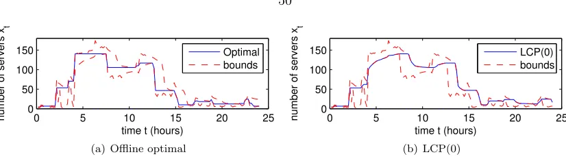
3.4 Lazy capacity provisioning . . . 50
3.5 Case studies . . . 51
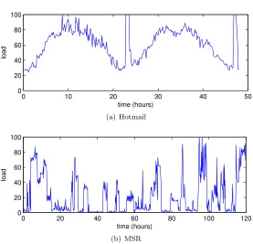
3.5.1 Experimental setup . . . 52
3.5.2 When is right-sizing beneficial? . . . 53
3.6 Concluding remarks . . . 59
Appendix 3.A Analysis of the offline optimal solution . . . 61
Appendix 3.B Analysis of lazy capacity provisioning, LCP(w) . . . 64
4 Cost-Effective Geographical Load Balancing 71 4.1 Model and notation . . . 73
4.1.1 The workload . . . 73
4.1.2 The Internet-scale system . . . 73
4.1.3 Cost optimization problem . . . 75
4.1.4 Generalizations . . . 76
4.2 Algorithms and analytical results . . . 77
4.2.1 Receding horizon control . . . 77
4.2.2 Fixed horizon control . . . 79
4.3 Case studies . . . 81
4.3.1 Experimental setup . . . 81
4.3.2 Experimental results . . . 84
4.4 Concluding remarks . . . 87
Appendix 4.A Notation . . . 88
Appendix 4.B Proof of Theorems 4.6 . . . 88
Appendix 4.C Proofs of Theorems 4.1 and 4.4 . . . 89
Appendix 4.D “Bad” instances for receding horizon control (RHC) . . . 91
5 Smoothed Online Convex Optimization 94 5.1 Problem formulation . . . 96
5.2 Background . . . 99
5.2.1 Online convex optimization . . . 99
5.2.2 Metrical task systems . . . 100
5.3 The incompatibility of regret and the competitive ratio . . . 101
5.5 Concluding remarks . . . 106
Appendix 5.A Proof of Proposition 5.1 . . . 107
Appendix 5.B Proof of Lemma 5.1 . . . 107
Appendix 5.C Proof of Lemma 5.2 . . . 108
Appendix 5.D Proof of Lemma 5.3 . . . 109
Appendix 5.E Proof of Lemma 5.4 . . . 110
Appendix 5.F Proof of Lemma 5.5 . . . 110
Chapter 1
Introduction
Data centers provide the supporting infrastructure for a wide range of IT services and consume a significant amount of electricity. According to the US EPA Report to the Congress on Server and Data Center Energy Efficiency in 2007, US data centers consume 61 billion kWh in 2006 (1.5% of total U.S. electricity). Moreover, it is growing exponentially at an annual rate of 15%. A recent report [76] revealed that although the growth rate slowed down a little recently, electricity used by data centers worldwide increased by about 56% from 2005 to 2010. Further, from an operator’s stand point, the energy cost has grown to exceed the server costs in data centers. Thus, it is not surprising that optimizing energy cost in data center is receiving increasing attention. However, saving energy and improving performance are usually in conflict with each other, and thus the joint optimization is a challenge.
1.1
Energy efficiency of data centers
may be more useful for servers.
For a data center, besides the energy consumed by the servers performing the computation, a large fraction of energy is consumed by the cooling and provisioning infrastructure. To capture this consumption, power usage effectiveness (PUE) measures the ratio of total building power to IT power, i.e., the power consumed by the actual computing equipments such as servers, network equipments and so on. It is reported that PUE was greater than 2 for typical data centers [52].
Fortunately, PUE can be substantially improved by careful design for energy efficiency. The most energy-efficient data centers today have PUE ≤ 1.2 [17]. This is achieved via a few steps (a) maintaining data centers at a higher temperature. It has been shown that increasing the cold aisle temperatures to 25-27◦C can save a large amount of cooling energy without causing higher equipment failures. (b) using more efficient air-flow control to reduce the energy needed for cooling. This is one of the primary reasons why container-based data centers are more efficient, because the hot air is isolated from the cold air and the path to the cooling coil is short. (c) adopting more efficient gear to reduce the UPS and power distribution losses. For example, using per-server UPSs instead of a facility-wide UPS will increase the efficiency of the overall power infrastructure by eliminating the AC-DC-AC overhead.
Beyond these engineering improvements, there is also significant energy reduction to be achieved via improved IT design in data centers [18, 3]. From the hardware perspective, according to [95], the main part of the power in a server is consumed by CPU, followed by the memory and the power loss. However, CPU no longer dominates the power consumption of the server. This is because the modern CPUs are adopting much more energy-efficient techniques than other system components. As a result, they can consume less than 30% of their peak power in low-activity mode, i.e., the dynamic power range is more than 70% of the peak power [16]. In contrast, the dynamic power ranges of all other components are much narrower: less than 50% for DRAM, 25% for disk drives, 15% for network switches, and negligible for other components. The energy efficiency of IT components has been widely studied from an algorithmic perspective as well. The goal here is usually to design energy-efficient algorithms that reduce energy consumption while minimizing compromise to service.
1.2
Algorithmic challenges in energy efficiency
servers. The optimization at the global data center level is to dispatch the workload across multiple data centers, considering electricity price diversity and propagation delay diversity. We focus on the algorithmic challenges at all three levels in this thesis.
At the server level, many energy-saving techniques developed for mobile devices directly benefit the design of energy-efficient servers such as power-down mechanism and speed-scaling technique. However, because of the activity pattern, speed-scaling technique is more useful than power-down mechanism for servers. The basic idea behind speed scaling is that running at a low speed consumes less energy. But running at a low speed will make the user delay increase. Thus the speed scaling algorithms need to make a tradeoff between performance and energy usage. Depending on the objective, we may want to minimize the energy usage while meeting job deadlines, optimize user experience given energy budget, or minimize a linear combination of user delay and energy usage.
At the local data center level, a guiding focus for research into ‘green’ data centers is the goal of designing data centers that are ‘power-proportional’, i.e., use power only in proportion to the load. However, current data centers are far from this goal – even today’s energy-efficient data centers consume almost half of their peak power when nearly idle [16]. A promising approach for making data centers more power-proportional is using software to dynamically adapt the number of active servers to match the current workload, i.e., to dynamically ‘right-size’ the data center. The algorithmic question is, how to determine how many servers to be active and how to control servers and requests.
At the global data center level, as the demand on Internet services has increased in recent years, enterprises have move to using several distributed data centers to provide better QoS for users. To improve user experience, they tend to disperse data centers geographically so that user requests from different regions can be routed to data centers nearby, thus reducing the propagation delay. Recently, since the energy cost is becoming a big fraction for the total cost of the data centers, it has been proposed that the energy costs, both monetary and environmental, can be reduced by exploiting temporal variations and shifting processing to data centers located in regions where energy currently has low cost. Lightly loaded data centers can then turn off surplus servers.
1.3
Overview of this thesis
This thesis is divided into four components. In Chapter 2 we focus on the speed scaling problem at the server level. In Chapter 3 we study the capacity management problem at the local data center level. In Chapter 4 we investigate the geographical load balancing problem at the global data center level. Finally, in Chapter 5 we move beyond the data center area and study a general optimization framework for online decision problems.1
Chapter 2: Server speed scaling
Algorithmic work at the server level focuses on designing algorithms to reduce energy consumption while minimizing compromise to performance. Most of the algorithms studied are online algorithms since the device has to decide which action to take at the current time without knowing the future. The algorithmic questions that have been studied most widely at the server level are power-down mechanisms and speed scaling. Our focus is on speed scaling algorithms, but we begin by briefly surveying power-down mechanisms.
Power-down mechanisms are widely used in mobile devices, e.g., laptop goes to sleep mode if it has been idle longer than a certain threshold. The design question is how to determine such idle thresholds. Generally, a device has multiple states, each state has its own power consumption rate, and it consumes a certain amount of energy to transit from one state to others. The device must be at active state to serve tasks, and it may go to some sleep states during idle periods to save energy. The goal is to minimize the total energy. It has been shown that the energy consumed by the best possible deterministic online algorithm is at most twice that of the optimal solution, and randomized algorithms can do even better [65]. Many generalizations of this problem have been studied, including stochastic settings [10].
Speed scaling is another way to save energy for variable speed devices, since running at a low speed consumes less energy. Fundamentally, a speed scaling algorithm must make two decisions at each time:(i) a scheduling policy must decide which job(s) to service, and (ii) a speed scaler must decide how fast to run the server. The analytic study of the speed scaling problem began with Yao et al. [124] in 1995. Since [124], three main performance objectives balancing energy and delay have been considered: (i) minimize the total energy used in order to meet job deadlines [14, 101], (ii) minimize the average response time given an energy budget [32, 125], and (iii) minimize a linear combination of expected response time and energy usage per job [4, 13].
improvements in speed scaling designs. Finally, our results uncover one unintended drawback of dynamic speed scaling: speed scaling can magnify unfairness.
The work presented in this chapter is based on the publications [7, 85].
Chapter 3: Dynamic capacity provisioning in data centers
Algorithmic questions at the local data center level focus on allocating compute resources for incom-ing workloads and dispatchincom-ing workloads in the data center. The goal of design is to achieve “energy proportionality” [16], i.e., use power only in proportion to the load. A promising approach for mak-ing data centers more power-proportional is to dynamically ‘right-size’ the data center. Specifically, dynamic right-sizing refers to adapting the way requests are dispatched to servers in the data center so that, during periods of low load, servers that are not needed do not have jobs routed to them and thus are allowed to enter power-saving modes (e.g., go to sleep or shut down).
Technologies that implement dynamic right-sizing are still far from standard in data centers due to a number of challenges. First, servers must be able to seamlessly transition into and out of power-saving modes while not losing their state. There has been a growing amount of research into enabling this in recent years, dealing with virtual machine state [39], network state [37] and storage state [108, 5]. Second, such techniques must prove to be reliable, since administrators may worry about wear-and-tear consequences of such technologies. Third, it is unclear how to determine how many servers to toggle into power-saving mode and how to control servers and requests.
We provide a new algorithm to address this third challenge. We develop a simple but general model that captures the major issues that affect the design of a right-sizing algorithm, including: the cost (lost revenue) associated with the increased delay from using fewer servers, the energy cost of maintaining an active server with a particular load, and the cost incurred from toggling a server into and out of a power-saving mode (including the delay, energy, and wear-and-tear costs). First, we analytically characterize the optimal solution. We prove that it exhibits a simple, ‘lazy’ structure when viewed in reverse time. Second, we introduce and analyze a novel, practical online algorithm motivated by this structure, and prove that this algorithm guarantees cost no larger than 3 times the optimal cost, under very general settings arbitrary workloads, and general delay cost and general energy cost models provided that they result in a convex operating cost. Further, in realistic settings its cost is nearly optimal. Additionally, the algorithm is simple to implement in practice and does not require significant computational overhead. Moreover, we contrast it with the more traditional approach of receding horizon control and show that our algorithm provides much more stable cost saving with general settings.
The work presented in this chapter is based on the publications [83].
Chapter 4: Cost-effective geographical load balancing
The algorithmic questions at the global data center level focus on exploring the diversity of power prices and the diversity of propagation delays given geographically distributed data centers. Further, electricity prices and workloads are time-varying, which makes the joint optimization on energy and performance even more challenging. There is a growing literature related to the energy optimization of geographic dispersed data centers, but is still a fairly open problem. So far, [104] investigates the problem of total electricity cost for data centers in multi-electricity-market environment and propose a linear programming formulation to approximate it. They consider the queueing delay constraint inside the data center (assumed to be anM/M/1 queue) but not the end-to-end delay of users, thus the diversity of propagation delay has not been explored. Another approach, DONAR [118] runs a simple, efficient algorithm to coordinate their replica-selection decisions for clients with the capacity at each data center fixed. The distributed algorithm solves an optimization problem that jointly considers both client performance and server load. However, DONAR does not optimize the capacity provision at each data center and thus does not explore the diversity of power price. Moreover, neither approach considers the time variation of power price and workloads in the optimization problem.
We developed a framework to jointly optimize the total energy cost and the end-to-end delay of users by considering the price diversity and delay diversity. Our goal is to find a global dispatching scheme to route the workload from different regions to certain data centers dynamically, while considering the capacity optimization at each data center. Similar to the energy optimization at the local data center level, we would like to optimize both the operating cost for providing the service and the switching cost for changing the provisioning in an online manner. A commonly suggested algorithm for this setting is “receding horizon control” (RHC), which computes the provisioning for the current time by optimizing over a window of predicted future loads. We show that RHC performs well in a homogeneous setting, in which all servers can serve all jobs equally well; however, we also prove that differences in propagation delays, servers, and electricity prices can cause RHC to perform badly. So, we introduce variants of RHC that are guaranteed to perform as well in the face of such heterogeneity.
understand what portfolio of renewable energy is most effective. The numerical results reveal that the optimal renewable portfolio may include more wind power than solar power, though solar power seems to have better correlation with the workload shape.
The work presented in this chapter is based on the publications [82, 88, 87].
Chapter 5: Smoothed online convex optimization
The optimization problems in Chapter 3 and Chapter 4 share a similar property: We would like to adapt our decision (e.g., capacity, routing) based on the time-varying environment (e.g., workload, electricity price, renewable availability), but we do not want to adapt it too frequently because changing the decisions incurs overhead (e.g., service migration, data movement, wear-and-tear con-sequence). Actually this property also exists in many other problems even outside of the data center environment. For example, video streaming [67], where the encoding quality of a video needs to change dynamically in response to network congestion, but where large changes in encoding quality are visually annoying to users; optical networking [126], in which there is a cost to reestablish a light path; and content placement problems for CDN, in which there is a cost to move data. In addition to applications within computer systems, there are a number of problems in industrial optimization having similar property. One is the dynamic dispatching of electricity generators, where a particu-lar portfolio of generation must be allocated to cover demand, but in addition to the time-varying operating costs of the generators there are significant “setup” and “ramping” costs associated with changing the generator output [69].
In this chapter we consider the general “smoothed online convex optimization” (SOCO) prob-lems, a variant of the class of online convex optimization (OCO) problems that is strongly related to metrical task systems. Actually, many applications typically modeled using online convex optimiza-tion have, in reality, some cost associated with a change of acoptimiza-tion; and so may be better modeled using SOCO rather than OCO. For example, OCO encodes the so-called “k-experts” problem, which has many applications where switching costs can be important, e.g., in stock portfolio management there is a cost associated with adjusting the stock portfolio owned. In fact, “switching costs” have long been considered important in related learning problems, such as the k-armed bandit problem which has a considerable literature studying algorithms that can learn effectively despite switching costs [9, 54]. Further, SOCO has applications even in contexts where there are no costs associated with switching actions. For example, if there is concept drift in a penalized estimation problem, then it is natural to make use of a regularizer (switching cost) term in order to control the speed of the drift of the estimator.
that this is due to a fundamental incompatibility between these two metrics – no algorithm (deter-ministic or randomized) can achieve sublinear regret and a constant competitive ratio, even in the case when the objective functions are linear. However, we also exhibit an algorithm that, for the im-portant special case of one-dimensional decision spaces, provides sublinear regret while maintaining a competitive ratio that grows arbitrarily slowly.
Chapter 2
Server Speed Scaling
Computer systems must make a fundamental tradeoff between performance and energy usage. The days of “faster is better” are gone — energy usage can no longer be ignored in designs, including chips and servers. The importance of energy has led the designs to move toward speed scaling. Speed scaling designs adapt the “speed” of the system so as to balance energy and performance measures. Speed scaling designs can be highly sophisticated — adapting the speed at all times to the current state (dynamic speed scaling) — or very simple — running at a static speed that is chosena priori
to balance energy and performance, except when idle (gated-static speed scaling).
The growing adoption of speed scaling designs for systems from chips to disks has spurred analytic research into the topic. The analytic study of the speed scaling problem began with Yao et al. [124] in 1995. Since [124], three main performance objectives balancing energy and delay have been considered: (i) minimize the total energy used in order to meet job deadlines, e.g., [14, 101] (ii) minimize the average response time given an energy/power budget, e.g., [32, 125], and (iii) minimize a linear combination of expected response time and energy usage per job [4, 13]. We focus on the third objective. This objective captures how much reduction in response time is necessary to justify using an extra 1 joule of energy, and naturally applies to settings where there is a known monetary cost to extra delay (e.g., many web applications). This is related to (ii) by duality.
Fundamentally, a speed scaling algorithm must make two decisions at each time: (i) ascheduling policy must decide which job(s) to service, and (ii) a speed scaler must decide how fast to run the server. It has been noted by prior work, e.g., [101], that an optimal speed scaling algorithm will use shortest remaining processing time (SRPT) scheduling. However, in real systems, it is often impossible to implement SRPT, since it requires exact knowledge of remaining sizes. Instead, typical system designs often use scheduling that is closer to processor sharing (PS), e.g., web servers, operating systems, and routers. We focus on the design of speed scalers for both SRPT and PS.
using a worst-case framework while the prior work for PS is done in a stochastic environment, the M/GI/1 queue.
Despite the considerable literature studying speed scaling, there are many fundamental issues in the design of speed scaling algorithms that are not yet understood. This work provides new insights into four of these issues:
I Can a speed scaling algorithm be optimal? What structure do (near-)optimal algorithms have?
II How does speed scaling interact with scheduling?
III How important is the sophistication of the speed scaler?
IV What are the drawbacks of speed scaling?
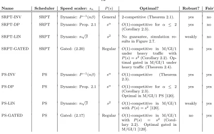
To address these questions we study both PS and SRPT scheduling under both dynamic and gated-static speed scaling algorithms. Our work provides (i) new results for dynamic speed scaling with SRPT scheduling in the worst-case model, (ii) the first results for dynamic speed scaling with PS scheduling in the worst-case model, (iii) the first results for dynamic speed scaling with SRPT scheduling in the stochastic model, (iv) the first results for gated-static speed scaling with SRPT in the stochastic model, and (v) the first results identifying unfairness in speed scaling designs. Table 2 summarizes these.
These results lead to important new insights into Issues I-IV above. We describe these insights informally here and provide pointers to the results in the body of the chapter.
With respect to Issue I, our results show that “energy-proportional” speed scaling provides near-optimal performance. Specifically, we consider the algorithm which uses SRPT scheduling and chooses sn, the speed to run at given n jobs, to satisfy P(sn) = nβ (where P(s) is the power
needed to run at speeds and 1/β is the cost of energy). We prove that this algorithm is (2 + ε)-competitive under general P (Corollary 2.1). This provides a tight analysis of an algorithm with a considerable literature, e.g., [4, 12, 13, 15, 81] (see Section 2.2.1 for a discussion). It also gives analytic justification for a common heuristic applied by system designers, e.g., [16]. Further, we show that no “natural” speed scaling algorithm (Definition 2.1) can be better than 2-competitive (Theorem 2.2), which implies that no online energy-proportional speed scaler can match the offline optimal.
With respect to Issue II, our results uncover two new insights. First, we prove that, at least with respect to PS and SRPT,speed scaling can be decoupled from the scheduler. That is, energy-proportional speed scaling performs well for both SRPT and PS (and another policy LAPS studied in [34]). Specifically, we show that PS scheduling with speeds such that P(sn) = n, which are
optimally competitive under SRPT, is again O(1)-competitive1 (Theorem 2.3). Further, we show
1O(·) ando(·) are defined in [20];f =ω(g)⇔g=o(f);f = Ω(g)⇔g=O(f);f = Θ(g)⇔[f =O(g) andg=
that using the speeds optimal for an M/GI/1 PS queue to control instead an M/GI/1 SRPT queue leads to nearly optimal performance (Section 2.2.2). Second, our results show that scheduling is not as important once energy is considered. Specifically, PS is O(1)-competitive for the linear combination of energy and response time; however, when just mean response time is considered PS is Ω(ν1/3)-competitive for instances withν jobs [96]. Similarly, we see in the stochastic environment
that the performance under SRPT and PS is almost indistinguishable (e.g., Figure 2.1). Together, the insights into Issue II provide a significant simplification of the design of speed scaling systems: they suggest that practitioners can separate two seemingly coupled design decisions and deal with each individually.
With respect toIssue III, our results add support to an insight suggested by prior work. Prior work [120] has shown that the optimal gated-static speed scaling algorithm performs nearly as well as the optimal dynamic speed scaling algorithm in the M/GI/1 PS setting. Our results show that the same holds for SRPT (Section 2.3). Thus, sophistication does not provide significant performance improvements in speed scaling designs. However, sophistication provides improved robustness (Sec-tion 2.4). To support this analytically, we provide worst-case guarantees on the (near) optimal stochastic speed scalers for PS and SRPT (Corollary 2.3). Note that it is rare to be able to provide such guarantees for stochastic control policies. The insights related to Issue III have an interesting practical implication: instead of designing “optimal” speeds it may be better to design “optimally robust” speeds, since the main function of dynamic speed scaling is to provide robustness. This represents a significant shift in approach for stochastic speed scaling design.
With respect to Issue IV, our results uncover one unintended drawback of dynamic speed scaling: speed scaling can magnify unfairness. Unfairness in speed scaling designs has not been identified previously, but in retrospect the intuition behind it is clear: If a job’s size is correlated with the occupancy of the system while it is in service, then dynamic speed scaling will lead to differential service rates across job sizes, and thus unfairness. We prove that speed scaling magnifies unfairness under SRPT (Theorem 2.5) and all non-preemptive policies, e.g., FCFS (Proposition 2.6). In contrast, PS is fair even with dynamic speed scaling (Proposition 2.5). Combining these results with our insights related to Issue II, we see that designers can decouple the scheduler and the speed scaler when considering performance, but should be wary about the interaction when considering fairness.
Name Scheduler Speed scaler: sn P(s) Optimal? Robust? Fair?
SRPT-INV SRPT Dynamic: P−1(nβ) General 2-competitive (Theorem 2.1). yes no
SRPT-DP SRPT Dynamic: Prop. 2.1 sα O(1)-competitive for α ≤ 2
(Corollary 2.3).
yes no
SRPT-LIN SRPT Dynamic: n√β s2 No guarantee, simulation re-sults in Figure 2.7.
weakly no
SRPT-GATED SRPT Gated: (2.20) Regular O(1)-competitive in M/GI/1 under heavy traffic with P(s) =s2(Corollary 2.2).
Op-timal gated in M/GI/1 under heavy traffic (Theorem 2.4).
no yes
PS-INV PS Dynamic: P−1(nβ) sα O(1)-competitive (Theorem
2.3).
yes yes
PS-DP PS Dynamic: Prop. 2.1 sα O(1)-competitive for α ≤ 2
(Corollary 2.3).
Optimal in M/GI/1 PS [120].
yes yes
PS-LIN PS Dynamic: n√β s2 O(1)-competitive in M/GI/1
withP(s) =s2[120].
weakly yes
PS-GATED PS Gated: (2.17) Regular O(1)-competitive in M/GI/1 with P(s) = s2
(Corol-lary 2.2). Optimal gated in M/GI/1 [120].
[image:20.612.111.553.61.338.2]no yes
Table 2.1: Summary of the speed scaling schemes in this chapter.
Thus, the policies considered in this chaptercan achieve any two of near-optimal, fair, and robust — but not all three.
Finally, it is important to note that the analytic approach in this chapter is distinctive. It is unusual to treat both stochastic and worst-case models together; and further, many results depend on a combination of worst-case and stochastic techniques, which leads to insights that could not have been attained by focusing on one model alone.
2.1
Model and notation
We consider the joint problem of speed scaling and scheduling in a single-server queue to minimize a linear combination of expected response time (also called sojourn time or flow time), denoted by T, and energy usage per job,E:
z=E[T] +E[E]/β. (2.1)
By Little’s law, this may be more conveniently expressed as
λz=E[N] +E[P]/β
Before defining the speed scaling algorithms, we need some notation. Letn(t) be the number of jobs in the system at timetands(t) be the speed that the system is running at timet. Further, define P(s) as the power needed to run at speeds. Then, the energy used by timetisE(t) =Rt
0P(s(τ))dτ.
Measurements have shown thatP(s) can take on a variety of forms depending on the system being studied; however, in many applications a low-order polynomial form provides a good approximation, i.e.,P(s) =ksαwith α∈(1,3). For example, for dynamic power in CMOS chipsα≈1.8 is a good approximation [120]. However, this polynomial form is not always appropriate. Some of our results assume a polynomial form to make the analysis tractable, and particularlyα= 2 provides a simple example which we use for many of our numerical experiments. Other results hold for general, even non-convex and discontinuous, power functions. Additionally, we occasionally limit our results to
regular power functions, which are differentiable on [0,∞), strictly convex, non-negative, and 0 at speed 0.
Now, we can define a speed scaling algorithm: A speed scaling algorithm A= (π,Σ), is a pair of a scheduling disciplineπthat defines the order in which jobs are processed, and a speed scaling rule Σ that defines the speed as a function of system state, in terms of the power function, P. In this chapter we consider speed scaling rules where the speed is a function of the number of jobs in the system, i.e.,sn is the speed when the occupancy isn.2
The scheduling algorithmsπwe consider are online, and so are not aware of a jobjuntil it arrives at timer(j), at which point πlearns the size of the job,xj. We consider a preempt-resume model,
that is, the scheduler may preempt a job and later restart it from the point it was interrupted without any overhead. The policies that we focus on are: shortest remaining processing time (SRPT), which preemptively serves the job with the least remaining work, and processor sharing (PS), which shares the service rate evenly among the jobs in the system at all times.
The speed scaling rules,sn, we consider can begated-static, which runs at a constant speed while
the system is non-idle and sleeps while the system is idle, i.e., sn = sgs1n6=0; or more generally dynamic sn =g(n) for some functiong:N∪ {0} →[0,∞). Note that the speed is simply the rate at which work is completed, i.e., a job of size xserved at speed s will complete in time x/s. To avoid confusion, we occasionally writesπn as the speed under policyπwhen the occupancy isn. The
queue is single-server in the sense that the full speedsn can be devoted to a single job.
We analyze the performance of speed scaling algorithms in two different models — one worst-case and one stochastic.
2This suits objective (2.1); e.g., it is optimal for an isolated batch arrival, and the optimalsis constant between
Notation for the worst-case model
In the worst-case model we consider finite, arbitrary (maybe adversarial) deterministic instances of arriving jobs. A problem instance consists of ν jobs, with thejth job having arrival time (release time) r(j) and size (work) xj. Our objective is again a linear combination of response time and
energy usage. LetE(I) be the total energy used to complete instanceI, andTjbe the response time
of jobj, the completion time minus the release time. The analog of (2.1) is to replace the ensemble average by the sample average, giving the cost of an instanceIunder a given algorithmAas
zA(I) = 1 ν
X
jTj+
1 βE(I)
.
In this model, we compare the cost of speed scaling algorithms to the cost of the optimal offline algorithm, OPT. In particular, we study the competitive ratio, defined as
CR= sup
I
zA(I)/zO(I),
wherezO(I) is the optimal cost achievable onI. A scheme is “c-competitive” if its competitive ratio is at mostc.
Notation for the stochastic model
In the stochastic model, we consider an M/GI/1 (or sometimes GI/GI/1) queue with arrival rate λ. LetX denote a random job size with c.d.f.F(x), c.c.d.f. ¯F(x), and continuous p.d.f.f(x). Let ρ=λE[X]∈[0,∞) denote the load of arriving jobs. Note thatρis not the utilization of the system and that many dynamic speed scaling algorithms are stable for allρ. When the power function is P(s) =sα, it is natural to use a scaled load,γ:=ρ/β1/α, which jointly characterizes the impact of
ρandβ (see [120]).
Denote the response time of a job of size xbyT(x). We consider the performance metric (2.1) where the expectations are averages per job. In this model the goal is to optimize this cost for a specific workload,ρ. Define the competitive ratio in the M/GI/1 model as
CR= sup
F,λ
zA/zO
2.2
Dynamic speed scaling
We start by studying the most sophisticated speed scaling algorithms, those that dynamically adjust the speed as a function of the queue length. In this section we investigate the structure of the “optimal” speed scaling algorithm in two ways: (i) we study near-optimal speed scaling rules in the case of both SRPT and PS scheduling; (ii) we study each of these algorithms in both the worst-case model and the stochastic model.
2.2.1
Worst-case analysis
There has been significant work studying speed scaling in the worst-case model, focusing on SRPT. A promising algorithm is (SRPT,P−1(n)), and there has been a stream upper bounds on its competi-tive ratio for objeccompeti-tive (2.1): for unit-size jobs in [4, 15] and for general jobs withP(s) =sαin [12, 81].
A major breakthrough was made in [13], which shows the 3-competitiveness of (SRP T, P−1(n+ 1)) for generalP.
Our contribution to this literature is twofold. First, we tightly characterize the competitive ratio of (SRPT,P−1(nβ)). Specifically, we prove that (SRPT,P−1(nβ)) is exactly 2-competitive under general power functions (see Theorem 2.1 and Corollary 2.1). Second, we prove that no “natural” speed scaling algorithm can be better than 2-competitive. Natural speed scaling algorithms include algorithms which have speeds that grow faster, slower, or proportional to P−1(nβ), or that use a scheduler that works on exactly one job between arrival/departure events (see Definition 2.1). Thus, the class of natural algorithms includes energy-proportional designs for all schedulers and SRPT scheduling for any sn. We conjecture that this result can be extended to all speed scaling
algorithms, which would imply that the competitive ratio of (SRPT,P−1(nβ)) is minimal.
In contrast to this stream of work studying SRPT, there has been no analysis of speed scaling under PS. We prove that (PS, P−1(nβ)) is O(1)-competitive for P(s) = sα with fixed α, and in
particular is (4α−2)-competitive for typicalα, i.e., α∈(1,3]. This builds on [34], which studies LAPS, another policy “blind” to job sizes. (LAPS,P−1(nβ)) is alsoO(1)-competitive in this case. For both PS and LAPS the competitive ratio is unbounded for largeα, which [34] proves holds for all blind policies. But, note thatα∈(1,3] in most computer systems today; thus, asymptotics inα are less important than the performance for smallα.
The results in this section highlight important insights about fundamental issues in speed scaling design. First, the competitive ratio results highlight that energy-proportional speed scaling (P(sn) =
nβ) is nearly optimal, which provides analytic justification of a common design heuristic, e.g., [16].
LAPS, we conjecture that it holds more generally. Third, scheduling seems much less important in the speed scaling model than in the standard constant speed model. For an instance of ν jobs, PS is Ω(ν1/3)-competitive for mean response time in the constant speed model [96], but is
O(1)-competitive in the speed scaling model. Again, we conjecture that this holds more generally than for just PS.
Amortized competitive analysis
The proofs of the results described above use a technique termedamortized local competitive analysis
[44, 107]. The technique works as follows.
To show that an algorithmAisc-competitive with an optimal algorithmOP T for a performance metricz=R
ζ(t)dtit is sufficient to find apotential function Φ :R→Rsuch that, for any instance of the problem:
1. Boundary condition: Φ = 0 before the first job is released, and Φ ≥ 0 after the last job is finished;
2. Jump condition: At any point where Φ is not differentiable, it does not increase; 3. Running condition: When Φ is differentiable,
ζA(t) +dΦ dt ≤cζ
O(t), (2.2)
where ζA(t) andζO(t) are the costζ(t) underAandOP T respectively.
Given these conditions, the competitiveness follows from integrating (2.2), which gives
zA≤zA+ Φ(∞)−Φ(−∞)≤czO.
SRPT analysis
We now state and prove our results for SRPT.
Theorem 2.1. For any regular power function P, (SRPT, P−1(nβ)) has a competitive ratio of exactly 2.
The proof of the upper bound is a refinement of the analysis in [13] that accounts more carefully for some boundary cases. It uses the potential function:
Φ(t) = Z ∞
0 n[q;t]
X
i=1
for some non-decreasing ∆(·) with ∆(i) = 0 fori≤0, wheren[q;t] = max(0, nA[q;t]−nO[q;t]) with
nA[q;t] andnO[q;t] the number of unfinished jobs at timetwith remaining size at leastqunder the
scheme under investigation and the optimal (offline) scheme, respectively.
The following technical lemma is the key step of the proof and is proven in Appendix 2.A.
Lemma 2.1. Let η≥1 andΦbe given by (2.3) with
∆(i) =1 +η β P
0 P−1(iβ)
. (2.4)
Let A= (SRP T, sn) withsn∈[P−1(nβ), P−1(ηnβ)]. Then at points where Φis differentiable,
nA+P(sA)/β+dΦ
dt ≤(1 +η)(n
O+P(sO)/β). (2.5)
Using the above Lemma, we can now prove Theorem 2.1.
Proof of Theorem 2.1. To show that the competitive ratio of (SRPT, P−1(nβ)) is at most 2, we show that Φ given by (2.3) and (2.4) is a valid potential function.
The boundary conditions are satisfied since Φ = 0 when there are no jobs in the system. Also, Φ is differentiable except when a job arrives or departs. When a job arrives, the change in nA[q]
equals that innO[q] for allq, and so Φ is unchanged. When a job is completed,n[q] is unchanged
for allq >0, and so Φ is again unchanged. The running condition is established by Lemma 2.1 with η= 1.
To prove the lower bound on the competitive ratio, consider periodic unit-work arrivals at rate λ=snfor somen. As the number of jobs that arrive grows large, the optimal schedule runs at rate
λ, and maintains a queue of at most one packet (the one in service), giving a cost per job of at most
(1 +P(λ)/β)/λ. In order to run at speed λ, the schedule (SRPT, P−1(nβ)) requires n =P(λ)/β jobs in the queue, giving a cost per job of (P(λ) +P(λ))/(λβ). The competitive ratio is thus at least β2+PP(λ(λ)). Asλbecomes large, this tends to 2 since a regularP is unbounded.
Theorem 2.1 can easily be extended to non-negative power functions by applying the same argument as used in [13].
Corollary 2.1. Let ε > 0. For any non-negative and unbounded P˜, there exists a P such that emulating (SRPT,P−1(nβ)) yields a (2 +ε)-competitive algorithm.
This emulation involves avoiding speeds where P is not convex, instead emulating such speeds by switching between a higher and lower speed on the convex hull of ˜P.
Definition 2.1. A speed scaling algorithmAisnaturalif it runs at speedsnwhen it hasnunfinished
jobs, and for convexP, one of the following holds:
(a) the scheduler is work-conserving and works on a single job between arrival/departure events; or
(b) g(s) +P(s)/β is convex, for someg with g(sn) =n; or (c) the speeds sn satisfy P(sn) =ω(n); or
(d) the speeds sn satisfy P(sn) =o(n).
This fragmented definition seems “unnatural”, the class contains most natural contenders for optimality: all algorithms that use the optimal scheduler SRPT, and all whose speeds grow faster than, slower than, or proportional to P−1(n). To be “unnatural”, an algorithm must have speeds which increase erratically (or decrease) asnincreases.
Theorem 2.2. For any ε >0 there is a regular power function Pε such that any natural algorithm Aon Pε has competitive ratio larger than 2−ε.
This theorem highlights that if an algorithm does have a smaller competitive ratio than (SRPT, P−1(nβ)), it will not use “natural” scheduling or speed scaling. Though the result only applies to natural algorithms, we conjecture that, in fact, it holds for all speed scaling algorithms, and thus the competitive ratio of (SRPT,P−1(nβ)) is minimal.
Proof. Consider the case whenP(s) =sα, withαyet to be determined. We show that, for largeα, the competitive ratio is at least 2−ε, by considering two cases: instanceIB(ν)is abatch arrival of
ν jobs of size 1 at time 0 with no future arrivals, and instanceIR(b,λ)is a batch ofb jobs at time 0
followed by a long train ofperiodic arrivals of jobs of size 1 at times k/λfork∈N.
Fix an ε >0 and consider a speed scaling which can attain a competitive ratio of 2−ε for all instances IR(·,·). For IR(·,λ), with largeλ, the optimal algorithm will run at speed exceedingλfor
a finite time until the occupancy is one. After that, it will run at speedλso that no queue forms. For long trains, this leads to a cost per job of (1 +P(λ)/β)/λ.
First, consider a “type (d)” naturalA. For sufficiently large λ, n > ksαn for allsn ≥λ/2, where
k= 2α+2/β. Between arrivals, at least 1/2 unit of work must be done at speed at leastλ/2, in order forAnot to fall behind. The cost per unit work is at least (1/s)(ksα+sα/β), and so the total cost of performing this 1/2 unit is at least (k+ 1/β)λα−1/2α >4λα−1/β. For largeλ, this is at least
twice the cost per job under the optimal scheme: (1 +P(λ)/β)/λ <2λα−1/β.
It remains to consider natural algorithms of types (a)–(c).
Consider a “type (a)” natural A on the instance IR(n,sn) for some n. It will initially process exactly one job at speed sn, which it will finish at time 1/sn. From this time, a new arrival will
last arrival. So, the average cost per job tends to (n+P(sn)/β)/sn on large instances, leading to a
competitive ratio of:
1 + n−1 P(sn)/β+ 1
≤CRperiodic≤2−ε. (2.6)
Consider a “type (b)” natural A. OnIR(n,sn), Aalso satisfies (2.6): Let ¯sto denote the time-average speed. For allφ <1, for sufficiently long instances we need ¯s≥φsnto prevent an unbounded
queue forming. By Jensen’s inequality, the average cost per job satisfies ¯z ≥ (g(¯s) +P(¯s)/β) ≥
(g(φsn) +P(φsn)/β). Since φ can be arbitrarily close to 1, the cost can be arbitrarily close to
n+P(sn)/β, implying (2.6).
For a “type (c)” natural A,P(sn)/n→ ∞for largen.
Thus, for types (a)–(c), ∃n0 such that for alln > n0:
sn≥ˆsn:=P−1
nβ
1−ε/2
. (2.7)
We now show that this condition precludes having a competitive ratio of 2−εin the case of batch arrivals,IB(ν).
ForIB(ν), the optimal strategy is to server one job at a time at some speedss∗n, giving cost
zO(IB(ν)) = ν X n=1 n s∗ n +P(s ∗ n) βs∗ n = ν X n=1
n(α−1)/α β1/α
" nβ (s∗
n)α
1/α +
(s∗n)α
nβ
(α−1)/α# .
The unique local minimum ofφ(·) = (·)(α−1)/α+ (·)−1/αoccurs at 1/(α−1). This gives a minimum cost of
zO(IB(ν)) =
αPν
n=1n (α−1)/α
β1/α(α−1)(α−1)/α
fors∗n= (nβ/(α−1))1/α. More generally, the optimum is
βn=s∗nP0(s∗n)−P(s∗n). (2.8)
Under A, when more thann−1 work remains, there must be at least nunfinished jobs. Thus, forα−1>1−ε/2,
z(IB(ν))≥ ν
X
n=n0
n(α−1)/α
β1/α
" nβ (ˆsn)α
1/α +
(ˆs
n)α
nβ
(α−1)/α# .
since the minimum ofφ(·) subject to (2.7) then occurs at (ˆsn)α/(nβ).
Since (ˆsn)α/(nβ) = 1/(1−ε/2), this gives
CRbatch≥
Pν n=n0n
(α−1)/α
Pν
n=1n(α−1)/α
!
(α−1)(α−1)/α
α
" 1 1−ε/2
(α−1)/α +
1
1−ε/2
For any ε∈(0,1), the product of the last two factors tends to 1 + 1/(1−ε/2) asα→ ∞, and hence there is anα=α(ε) for which their product exceeds 1/(1−ε/3) + 1. Similarly, for allα >1, there is a sufficiently largeνthat the first factor exceeds 1/(1 +ε/9). For thisαandν,CRbatch>2.
So, for P(s) =sα(ε), if the competitive ratio is smaller than 2−εin the periodic case, it must
be larger than 2 in the batch case.
Theorem 2.2 relies on P being highly convex, as in interference-limited systems [58]. For CMOS systems in which typicallyα∈(1,3], it is possible to design natural algorithms that can outperform (SRPT,P−1(nβ)).
PS analysis
We now state and prove our bound on the competitive ratio of PS.
Theorem 2.3. If P(s) =sα then (PS, P−1(nβ)) is max(4α−2,2(2−1/α)α)-competitive.
In particular, PS is (4α−2)-competitive forαin the typical range of (1,3].
Theorem 2.3 is proven using amortized local competitiveness. Let η≥1, and Γ = (1 +η)(2α−
1)/β1/α. The potential function is then defined as
Φ = Γ
nA(t) X
i=1
i1−1/αmax(0, qA(ji;t)−qO(ji;t)) (2.9)
whereqπ(j;t) is the remaining work on jobjat timetunder schemeπ, and{ji} nA(t)
i=1 is an ordering
of the jobs in increasing order of release time: r(j1)≤r(j2)≤ · · · ≤r(jnA(t)). Note that this is a scaling of the potential function that was used in [34] to analyze LAPS. As a result, to prove Theorem 2.3, we can use the corresponding results in [34] to verify the boundary and jump conditions. All that remains is the running condition, which follows from the technical lemma below. The proof is provided in Appendix 2.B.
Lemma 2.2. LetΦbe given by (2.9) andAbe the discipline (PS,sn) withsn ∈[(nβ)1/α,(ηnβ)1/α]. Then under A, at points whereΦis differentiable,
nA+ (sA)α/β+dΦ dt ≤c(n
O+ (sO)α/β) (2.10)
wherec= (1 +η) max((2α−1),(2−1/α)α).
2.2.2
Stochastic analysis
In a real application, it is clear that incorporating knowledge about the workload into the design can lead to improved performance. Of course, the drawback is that there is always uncertainty about workload information, either due to time-varying workloads, measurement noise, or simply model inaccuracies. We discuss robustness to these factors in Section 2.4, and in the current section assume that exact workload information is known to the speed scaler and that the model is accurate.
In this setting, there has been a substantial amount of work studying the M/GI/1 PS model [30, 42, 48, 117]3. This work is in the context of operations management and so focuses on “operat-ing costs” rather than “energy”, but the model structure is equivalent. This series of work formulates the determination of the optimal speeds as a stochastic dynamic programming (DP) problem and provides numeric techniques for determining the optimal speeds, as well as proving that the op-timal speeds are monotonic in the queue length. The opop-timal speeds have been characterized as follows [120]. Recall thatγ=ρ/β1/α.
Proposition 2.1. Consider an M/GI/1 PS queue with controllable service ratessn. LetP(s) =sα.
The optimal dynamic speeds are concave and satisfy the dynamic program given in [120]. Forα= 2
and any n≥2γ, they satisfy
γ+pn−2γ≤ √sn
β ≤γ+
√
n+ min γ 2n, γ
1/3. (2.11)
For generalα >1, they satisfy4
sn
β1/α ≤
1 αminσ>γ
n+σα−γα
(σ−γ) + γ (σ−γ)2
1/(α−1)
(2.12) sn
β1/α ≥
n
α−1 1/α
. (2.13)
Proof. Bounds (2.11) and (2.12) are shown in [120]. Additionally, the concavity ofsn follows from
results in [120]. To prove (2.13), note that whenρ= 0 the optimal speeds are those optimal for batch arrivals, which satisfy (2.13) by (2.8). Then, it is straightforward from the DP that sn increases
monotonically with loadρ, which gives (2.13).
Interestingly, the bounds in Proposition 2.1 are tight for large nand have a form similar to the form of the worst-case speeds for SRPT and PS in Theorems 2.1 and 2.3.
In contrast to the large body of work studying the optimal speeds under PS scheduling, there is no work characterizing the optimal speeds under SRPT scheduling. This is not unexpected since the analysis of SRPT in the static speed setting is significantly more involved than that of PS. Thus, instead of analytically determining the optimal speeds for SRPT, we are left to use a heuristic
3These actually study the M/M/1 FCFS queue, but since the M/GI/1 PS queue with controllable service rates is
a symmetric discipline [72] it has the same occupancy distribution and mean delay as an M/M/1 FCFS queue.
approach.
Note that the speeds suggested by the worst-case results for SRPT and PS (Theorems 2.1 and 2.3) are the same, and the optimal speeds for a batch arrival are given by (2.8) for both policies. Motivated by this and the fact that (2.8) matches the asymptotic form of the stochastic results for PS in Proposition 2.1,we propose to use the optimal PS speeds in the case of SRPT.
To evaluate the performance of this heuristic, we use simulation experiments (Figure 2.1) that compare the performance of this speed scaling algorithm to the following lower bound.
Proposition 2.2. In a GI/GI/1 queue withP(s) =sα,
zO≥ 1
λmax(γ
α, γα(α−1)(1/α)−1).
This was proven in [120] in the context of the M/GI/1 PS but the proof can easily be seen to hold more generally.
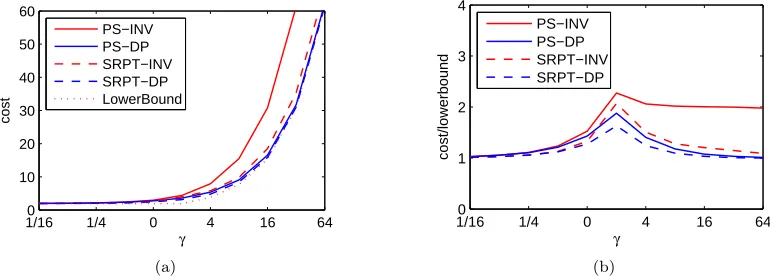
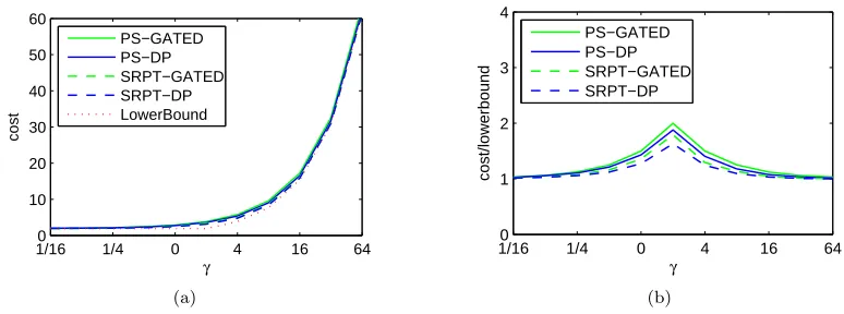
Simulation experiments also allow us to study other interesting topics, such as (i) a comparison of the performance of the worst-case schemes for SRPT and PS with the stochastic schemes and (ii) a comparison of the performance of SRPT and PS in the speed scaling model. In these experiments, the optimal speeds for PS in the stochastic model are found using the numeric algorithm for solving the DP described in [48, 120], and then these speeds are also used for SRPT. Due to limited space, we describe the results from only one of many settings we investigated.
Figure 2.2 shows that the optimal speeds from the DP (“DP”) have a similar form to the speeds motivated by the worst-case results, P−1(nβ) (“INV”), differing byγ for high queue occupancies. Figure 2.1 shows how the total cost (2.1) depends on the choice of speeds and scheduler. At low loads, all schemes are indistinguishable. At higher loads, the performance of the PS-INV scheme degrades significantly, but the SRPT-INV scheme maintains fairly good performance. Note though that if P(s) =sαforα >3 the performance of SRPT-INV degrades significantly too. In contrast, the
DP-based schemes benefit significantly from having the slightly higher speeds chosen to optimize (2.1) rather than minimize the competitive ratio. Finally, the SRPT-DP scheme performs nearly opti-mally, which justifies the heuristic of using the optimal speeds for PS in the case of SRPT5. However, the PS-DP scheme performs nearly as well as SRPT-DP. Together, these observations suggest that it is important to optimize the speed scaler, but not necessarily the scheduler.
2.3
Gated-static speed scaling
Section 2.2 studied a sophisticated form of speed scaling where the speed can depend on the current occupancy. This scheme can perform (nearly) optimally; however its complexity and overheads may
1/160 1/4 0 4 16 64 10
20 30 40 50 60
γ
cost
PS−INV PS−DP SRPT−INV SRPT−DP LowerBound
(a)
1/160 1/4 0 4 16 64
1 2 3 4
γ
cost/lowerbound
PS−INV PS−DP SRPT−INV SRPT−DP
[image:31.612.130.515.84.223.2](b)
Figure 2.1: Comparison of SRPT and PS scheduling under bothsn=P−1(nβ) and speeds optimized
for an M/GI/1 PS system, using Pareto(2.2) job sizes andP(s) =s2.
be prohibitive. This is in contrast to the simplest non-trivial form: gated-staticspeed scaling, where sn=sgs1n6=0for some constant speedsgs. This requires minimal hardware to support; e.g., a CMOS
chip may have a constant clock speed but AND it with the gating signal to set the speed to 0. Gated-static speed scaling can be arbitrarily bad in the worst case since jobs can arrive faster thansgs. Thus, we study gated-static speed scaling only in the stochastic model, where the constant
speedsgs can depend on the load.
We study the static speed scaling under SRPT and PS scheduling. The optimal gated-static speed under PS has been derived in [120], but the optimal speed under SRPT has not been studied previously.
Our results highlight two practical insights. First, we show that gated-static speed scaling can provide nearly the same cost as the optimal dynamic policy in the stochastic model. Thus, the simplest policy can nearly match the performance of the most sophisticated policy. Second, we show that the performance of gated-static under PS and SRPT is not too different, thus scheduling is much less important to optimize than in systems in which the speed is fixed in advance. This reinforces what we observed for dynamic speed scaling.
2.3.1
Optimal gated-static speeds
We now derive the optimal speed sgs, which minimizes the expected cost of gated-static in the
stochastic model under both SRPT and PS. First note that, since the power cost is constant at P(sgs) whenever the server is running, the optimal speed is
sgs= arg min
s βE[T] +
1
0 20 40 60 80 100 0
2 4 6 8 10 12
n s n
[image:32.612.354.520.73.196.2]DP INV
Figure 2.2: Comparison of sn =P−1(nβ) with
speeds “DP” optimized for an M/GI/1 system withγ= 1 andP(s) =s2.
0.5 0.9 0.99 0.999
0 10 20 30 40
ρ
E[T]
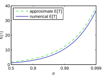
[image:32.612.128.294.76.194.2]approximate E[T] numerical E[T]
Figure 2.3: Validation of the heavy-traffic approximation (2.19) by simulation using Pareto(3) job sizes withE[X] = 1.
In the second term Pr(N 6= 0) =ρ/s, and so multiplying byλand setting the derivative to 0 gives that the optimal gated-static speed satisfies
βdE[N] ds +r
P∗(s)
s = 0, (2.15)
wherer=ρ/sis the utilization and
P∗(s)≡sP0(s)−P(s). (2.16)
Note that if P is convex then P∗ is increasing and if P00 is bounded away from 0 then P∗ is unbounded.
Under PS, E[N] = ρ/(s−ρ), and sodE[N]/ds =E[N]/(ρ−s). By (2.15), the optimal speeds satisfy [120]
βE[N] = (1−r)rP∗(s). (2.17)
Unfortunately, in the case of SRPT, things are not as easy. Fors= 1, it is well known, e.g., [75], that
E[T] = Z ∞
x=0
Z x
t=0
dt 1−λRt
0τ dF(τ)
+λ Rx
0 τ 2
dF(τ) +x2F¯(x) 2(1−λR0xτ dF(τ))2 dF(x)
The complexity of this equation rules out calculating the speeds analytically. So, instead we use simpler forms forE[N] that are exact in asymptotically heavy or light traffic.
A heavy-traffic approximation
We state the heavy-traffic results for distributions whose c.c.d.f. ¯Fhas lower and upper Matuszewska indices [20] ofm and M. Intuitively, C1xm .F(x)¯ .C2xM as x→ ∞ for some C1, C2. So, the
be the fraction of work coming from jobs of size at mostx. The following was proven in [85].
Proposition 2.3 ([85]). For an M/GI/1 under SRPT with speed 1, E[N] = Θ(H(ρ)) as ρ→ 1, where
H(ρ) =
E[X2]/((1−ρ)G−1(ρ)) if M <−2
E[X] log(1/(1−ρ)) if m >−2.
(2.18)
Proposition 2.3 motivates the heavy-traffic approximation below for the case when the speed is 1:
E[N]≈CH(ρ) (2.19)
whereC is a constant dependent on the job size distribution. For job sizes which are Pareto(a) (or more generally, regularly varying [20]) with a >2, it is known thatC = (π/(1−a))/(2 sin(π/(1−
a))) [85]. Figure 2.3 shows that in this case, the heavy-traffic results are accurate even for quite low
loads.
Given approximation (2.19), we can now return to equation (2.15) and calculate the optimal speed for gated-static SRPT. Defineh(r) = (G−1)0(r)/G−1(r).
Theorem 2.4. Suppose approximation (2.19) holds with equality.
(i) IfM <−2, then for the optimal gated-static speed,
βE[N]
2−r
1−r −rh(r)
=rP∗(s). (2.20a)
(ii) Ifm >−2, then for the optimal gated-static speed,
βE[N]
1
(1−r) log(1/(1−r))
=P∗(s). (2.20b)
Proof. For brevity, we only prove the second claim. Ifm >−2, then there is aC0=CE[X] such that
E[N] =
C0 s log
1
1−ρ/s
. (2.21)
for speeds. Now
dE[N] ds =−
C0 s2 log
1
1−ρ/s
− C
0ρ
s2(s−ρ)
=−E[N]
s
1 + ρ s
1
(1−ρ/s) log(1/(1−ρ/s))
,
1 2 4 8 16 32 0
0.2 0.4 0.6 0.8 1
ρ
ρ
/s
PS−GATED SRPT−GATED
(a)
2 3 4 5
9 9.5 10 10.5 11 11.5
a
s
PS−GATED SRPT−GATED
[image:34.612.132.517.79.222.2](b)
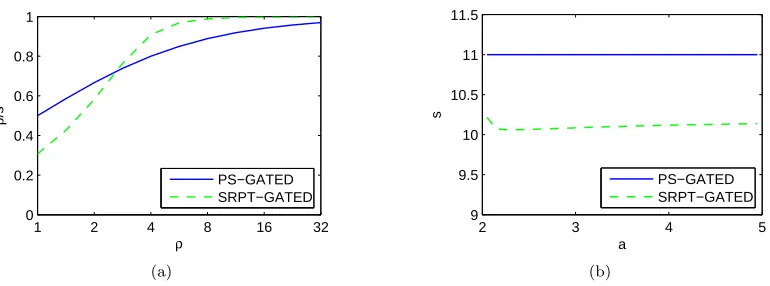
Figure 2.4: Comparison for gated-static: PS using (2.17) and SRPT using (2.22), withP(s) =s2.
(a) Utilization given Pareto(2.2) job sizes. (b) Dependence of speed on the job size distribution, for Pareto(a).
To evaluate the speeds derived for heavy-traffic, Figure 2.4(b) illustrates the gated-static speeds derived for SRPT and PS, forP(s) =s2andρ= 10 and varying job size distribution. This suggests that the SRPT speeds are nearly independent of the job size distribution. (Note that the vertical axis does not start from 0.) Moreover, the speeds of SRPT and PS differ significantly in this setting since the speeds under SRPT are approximately minimal (the speeds must be larger thanγ), while the PS speeds areγ+ 1.
Beyond heavy-traffic regime
Let us next briefly consider the light-traffic regime. Asρ→0, there is seldom more than one job in the system, and SRPT and PS have nearly indistinguishableE[N]. So, in this case, it is appropriate to use speeds given by (2.17).
Given the light-traffic and heavy-traffic approximations we have just described, it remains to decide the speed in the intermediate regime. We propose setting
sSRP Tgs = min(sP Sgs , sSRP Tgs (HT)), (2.22)
wheresP S
gs satisfies (2.17), ands
SRP T(HT)
gs is given by (2.20) withE[N] estimated by (2.19). To see why (2.22) is reasonable, we first show that (2.20) often tends to the optimal speed as ρ→0.
Proposition 2.4. If m >−2 or bothM <−2 and arbitrarily small jobs are possible (i.e., for all
1/160 1/4 0 4 16 64 10
20 30 40 50 60
γ
cost
PS−GATED PS−DP SRPT−GATED SRPT−DP LowerBound
(a)
1/160 1/4 0 4 16 64
1 2 3 4
γ
cost/lowerbound
PS−GATED PS−DP SRPT−GATED SRPT−DP
[image:35.612.128.515.81.225.2](b)
Figure 2.5: Comparison of PS and SRPT with gated-static speeds (2.17) and (2.22), versus the dynamic speeds optimal for an M/GI/1 PS. Job sizes are distributed as Pareto(2.2) andP(s) =s2.
From (2.8), this is the optimal speed at which to server a batch of a single job. Since, asρ→0, the system almost certainly has a single job when it is non-empty, this is an appropriate speed.
Although (2.20) tends to the optimal speeds, (2.19) over estimates E[N] for small ρ and so sSRP Tgs (HT) is higher than optimal for small loads. Conversely, for a given speed, the delay is less
under SRPT than PS, and so the optimal speed under SRPT will be lower than that under PS. Hence sSRP Tgs (HT)< sP Sgs in the largeρregime where the former becomes accurate. Thus, the min
operation in (2.22) selects the appropriate form in each regime.
2.3.2
Gated-static vs. dynamic speed scaling
Now that we have derived the optimal static speeds, we can contrast the performance of gated-static with that of dynamic speed scaling. This is a comparison of the most and least sophisticated forms of speed scaling.
As Figure 2.5 shows, the performance (in terms of mean delay plus mean energy) of a well-tuned gated-static system is almost indistinguishable from that of the optimal dynamic speeds. Moreover, there is little difference between the cost under PS-GATED and SRPT-GATED, again highlighting that the importance of scheduling in the speed scaling model is considerably less than in standard queueing models.
In addition to observing numerically that the gated-static schemes are near optimal, it is possible to provide some analytic support for this fact as well. In [120] it was proven that PS-GATED is within a factor of 2 of PS-DP when P(s) =s2. Combining this result with the competitive ratio
results, we have
0 10 20 30 40 5
10 15 20
design γ
cost
SRPT−GATED SRPT−DP SRPT−LIN
(a) SRPT
0 10 20 30 40
5 10 15 20
design γ
cost
PS−GATED PS−DP PS−LIN
[image:36.612.133.518.73.221.2](b) PS
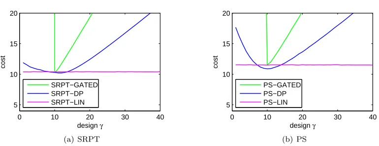
Figure 2.6: Effect of misestimatingγ under PS and SRPT: cost whenγ = 10, but sn are optimal
for a different “designγ”. Pareto(2.2) job sizes;P(s) =s2.
Proof. Letπ∈ {P S, SRP T}andsπ
gsbe the optimal gated-static speed forπandsDPn be the optimal
speeds, which solve the DP for the M/GI/1 PS queue. Then
z(π,sπgs)≤z(P S,s P S
gs)≤2z(P S,s DP
n )≤2z(P S,P
−1(nβ))
≤12zO.
The last three steps follow from [120], the optimality of DP for PS in M/GI/1, and Theorem 2.3.
2.4
Robustness and speed scaling
Section 2.3 shows that near-optimal performance can be obtained using the simplest form of speed scaling — running at a static speed when not idle. Why then do CPU manufacturers design chips with multiple speeds? The reason is that the optimal gated-static design depends intimately on the loadρ. This cannot be known exactly in advance, especially since workloads typically vary over time. So, an important property of a speed scaling design isrobustness to uncertainty in the workload,ρ andF, and to model inaccuracies.
Figure 2.6 illustrates that if a gated-static design is used, performance degrades dramatically when ρ is mispredicted. If the static speed is chosen and the load is lower than expected, excess energy will be used. Underestimating the load is even worse; if the system has static speeds and ρ≥sthen the cost is unbounded.
In contrast, Figure 2.6 illustrates simulation experiments which show that dynamic speed scaling (SRPT-DP) is significantly more robust to misprediction of the workload. In fact, we can prove this analytically by providing worst-case guarantees for the SRPT-DP and PS-DP. LetsDP
n denote the
Corollary 2.3. Consider P(s) = sα with6 α∈ (1,2] and algorithm A which chooses speeds sDP n
optimal for PS scheduling in an M/GI/1 queue with loadρ. IfAuses either PS or SRPT scheduling,
thenA isO(1)-competitive in the worst-case model.
Proof. The proof applies Lemmas 2.1 and 2.2 from the worst-case model to the speeds from the stochastic model.
By Proposition 2.1, sn ≥(nβ/(α−1))1/α. Since α < 2, this implies sn ≥P−1(nβ). Further,
(2.12) implies thatsDPn =O(n1/α) for any fixedρandβ and is bounded for finite n.
Hence the speedssDPn are of the form given in Lemmas 2.1 and 2.2 for some finiteη (dependent
onπand the constantρ), from which it follows thatAis constant competitive. For α= 2, Proposition 2.1 impliessDP
n ≤(2γ+ 1)P−1(nβ), whence (SRPT, sDPn ) is (2γ+
2)-competitive.
Corollary 2.3 highlights thatsDP
n designed for a givenρleads to a speed scaler that is “robust”.
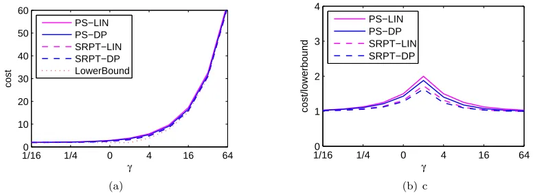
However, the cost still degrades significantly whenρis mispredicted badly (as shown in Figure 2.6). We now consider a different form of robustness: If the arrivals are known to be well approximated by a Poisson process, butρis unknown, is it possible to choose speeds that are close to optimal for allρ? It was shown in [120] that using “linear” speeds,sn=n
√
β, gives near-optimal performance
whenP(s) =s2and PS scheduling is used. This scheme (“LIN”) performs much better than using sn=P−1(nβ), despite the fact that it also uses no knowledge of the workload. Given the decoupling
of scheduling and speed scaling suggested by the results in Section 2.2, this motivates using the same linear speed scaling for SRPT. Figure 2.7 illustrates that this linear speed scaling provides near-optimal performance under SRPT too. The robustness of this speed scaling is illustrated in Figure 2.6. However, despite being more robust in the sense of this paragraph, the linear scaling is not robust to model inaccuracies. Specifically, it is notO(1)-competitive in general, nor even for the case of batch arrivals.
2.5
Fairness and speed scaling
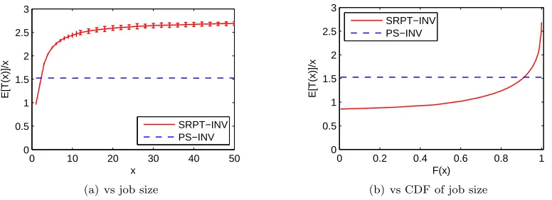
To this point we have seen that speed scaling has many benefits; however we show in this section that dynamic speed scaling has an undesirable consequence — magnifying unfairness. Fairness is an important concern for system design in many applications, and the importance of fairness when considering energy efficiency was recently raised in [109]. However, unfairness under speed scaling designs has not previously been identified. In retrospect though, it is not a surprising byproduct of speed scaling: If there is some job type that is always served when the queue length is long/short it will receive better/worse performance than it would have in a system with a static speed. To see
1/160 1/4 0 4 16 64 10
20 30 40 50 60
γ
cost
PS−LIN PS−DP SRPT−LIN SRPT−DP LowerBound
(a)
1/160 1/4 0 4 16 64
1 2 3 4
γ
cost/lowerbound
PS−LIN PS−DP SRPT−LIN SRPT−DP
[image:38.612.130.518.82.224.2](b) c
Figure 2.7: Comparison of PS and SRPT with linear speeds,sn =n √
β, and with dynamic speeds optimal for PS. Job sizes are Pareto(2.2) andP(s) =s2.
that this magnifies unfairness, rather than being independent of other biases, note that the scheduler has greatest flexibility to select which job to serve when the queue is long, and so jobs served at that time are likely to be those that already get better service.
In this section, we prove that this service rate differential can lead to unfairness in a rigorous sense under SRPT and non-preemptive policies such as f