Large eddy simulation of molecular mixing in a recirculating shear flow

(1)

Large-Eddy Simulation of Molecular Mixing in a

Recirculating Shear Flow

Thesis by

Georgios Matheou

In Partial Fulfillment of the Requirements for the Degree of

Doctor of Philosophy

California Institute of Technology Pasadena, California

2008

(2)

(3)

(4)

Acknowledgements

I would like to express my deepest appreciation towards my advisor, Professor Paul Dimotakis, for his mentorship, guidance, and support during my time at Caltech. This work would not have been made possible without his efforts to provide essential resources. My gratitude also extends to the other members of my committee, Professors Tim Colonius, Daniel Meiron, Dale Pullin, and Joseph Shepherd, for their suggestions and constructive criticism of the thesis.

I am also indebted to Professor Carlos Pantano, who has been a great (and patient) mentor. I would like to thank Carlos Pantano, David Hill, and Ralf Deiterding for their assistance with the VTF/AMROC computational framework, and for developing and maintaining this tool.

Aristides Bonanos, Jeff Bergthorson, and Michael Johnson provided the experimental measure-ments used in the simulations presented in this thesis. I would like to thank them for their assistance with the experimental data and the numerous discussions that improved the quality of this work.

I would also like to acknowledge discussions with the members of the GALCIT community and the Compressible Turbulence group that was part of the Caltech Advanced Simulation and Computing (ASC) program. I would especially like to thank Kazuo Sone, Antonino Ferrante, and Daniel Appel¨o for discussions on numerical analysis and computer science issues. Computer support by Dan Lang and administrative support by Christina Mojahedi at Professor Dimotakis’ group are also appreciated. I would like to thank the Center for Advanced Computing Research at Caltech and the Livermore Computing Center at Lawrence Livermore National Laboratory for technical assistance.

This work was supported by AFOSR Grants 04-1-0020, 04-1-0389, and FA9550-07-1-0091, by the Caltech DOE Advanced Simulation and Computing (ASC) Alliance Center under subcontract No. B341492 of DOE contract W-7405-ENG-48, and NSF Grant EIA-0079871.

During my time at Caltech I have met many friends who have made this experience more enjoy-able and rewarding. In particular, I would like to thank (in the order I met them) Fotini Liepouri, George Lykotrafitis, Melania Apostolidou, Aristides Bonanos, and Benjamin Sexson.

(5)

Abstract

The flow field and mixing in an expansion-ramp geometry is studied using large-eddy simulation (LES) with subgrid scale (SGS) modeling based on the stretched-vortex model for momentum and scalar subgrid turbulent transport. The expansion-ramp geometry was developed to provide enhanced mixing and flameholding characteristics while maintaining low total-pressure losses, ele-ments that are important in the design and performance of combustors for hypersonic air-breathing propulsion applications. In the expansion ramp configuration considered in this study, a subsonic top stream is expanded over a perforated ramp at an angle of 30◦_{through which a secondary stream}

is injected. The separation of the top stream creates a shear layer that reattaches on the lower wall when the mass flux of the lower stream is insufficient to provide the entrainment requirements, in a similar manner to a backward-facing step configuration. Depending on the mass-flux ratio of the two streams the shear layer splits at reattachment, and part of the flow is deflected upstream forming a re-entrant jet within the recirculation zone, resulting in enhanced mixing and flameholding.

The approach followed in this work relies on verification and validation of the numerical methods and turbulence models, focusing on development of a truly predictive computational framework for turbulent-mixing applications. The mixing was studied by tracking a passive scalar without taking into account the effects of chemical reactions and heat release, an approximation expected to be adequate in experiments conducted in parallel. The numerical methodology employs non-dissipative approximations of the spatial derivatives and a turbulence model based on physical arguments. No turbulence-model parameters were adjusted in the simulations.

(6)

shear layer is found to be in agreement with the prediction of the LSA.

The flow and mixing predictions of the LES are in good agreement with experimental measure-ments in the expansion-ramp geometry. Specifically, the recirculating flow between the ramp and the reattachment of the shear layer is reproduced by the LES. The magnitude of the velocity of upstream-moving flow near the lower wall is 10–15% of the top free stream for mass-injection ratios of about 1/10, but becomes negligible as the flow tends towards a free shear layer, for higher mass-injection ratios of about 1/5. The mean reattachment length of the primary shear layer is somewhat overpredicted by the simulations for all the cases studied. The agreement in the pressure coefficient profiles along the top and bottom walls and the total pressure profiles along the transverse direction is satisfactory.

Total (resolved and subgrid) probability density functions (PDFs) of the scalar are estimated using an assumed beta-distribution model for the subgrid scalar field. The improved mixing charac-teristics of the geometry compared to free shear layers at equivalent conditions are illustrated by the shapes of the PDFs. Moreover, the temperature rise and the probability of mixed fluid profiles are in good agreement with the experimental measurements, indicating that the mixing on a molecular scale is correctly predicted by the LES–SGS model.

(7)

List of Figures

1.1 Schematic of the expansion-ramp geometry. The top stream,U1, enters the test section

in the horizontal direction while the lower stream,UR, is injected through a perforated

ramp at α= 30◦_{. The separating top stream forms the primary shear layer, which}

reattaches downstream (not pictured) with part of the flow being deflected upstream in the recirculation region. The upstream moving fluid forms a secondary shear layer where the ramp meets the lower guide wall. . . 4 1.2 Schlieren visualization of the flow in the expansion ramp geometry from the experiments

of Johnson (2005). The primary and secondary shear layers are clearly visible. Upper stream U1 ≈120 m/s, lower steam UR ≈ 5.5 m/s. Upper stream composition is N2

and lower stream is 66.66% Ar, 33.33% He (non-reacting flow). . . 6 1.3 Schlieren visualization of the flow in the expansion ramp geometry from the experiments

of Johnson (2005). Upper stream U1 ≈120 m/s, lower steamUR ≈12.5 m/s. Upper

stream composition is N2 and lower stream is 66.66% Ar, 33.33% He (non-reacting

flow). The increased injection pushes the recirculation zone downstream eliminating the secondary mixing layer (cf. Fig. 1.2). . . 6

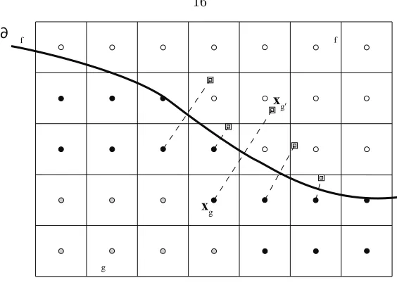
2.1 Schematic showing a two-dimensional computational grid intersected by a level set de-fined boundary, ∂Ωf (thicker line). The grid is divided in two regions, the physical

domain (Ωf) and the ghost fluid (Ωg). Filled black circles denote the band of cells

ad-jacent to the boundary that have to be populated by the ghost fluid method, assuming here that the width of the stencil is 5 cells. The mirror points,xg0, ofx_g, with respect to the boundary, are also shown (squares) for some of the ghost cells. . . 16

3.1 L1 and L∞ norm of the error versus grid spacing for mass, momentum, energy, and

mixture fraction for the vortex test case with periodic boundary conditions . . . 22 3.2 L1 norm of the density error versus time for a grid resolution of 256×256. A unit of

normalized timet/trcorresponds to about one vortex revolution. . . 22

(10)

3.4 Streamwise velocity perturbation fields. The panel on the left depicts the linear stability analysis prediction and the one on the right the computed field for Case A, ∆x= 0.0625 andt= 20. Note the exponential growth of the perturbation. . . 30 3.5 L∞ norm of the error versus grid spacing for Shear Layer A (left) and B att = 20.

Solid lines correspond to the error norm of the streamwise velocity perturbation, u0_,

and dashed to the transverse, v0_{. The error for Shear Layer A tends to a constant as}

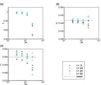
grid spacing decreases due to a mismatch in the growth rate with the linear stability analysis prediction. Perturbations in Case B grow at the expected rate and the error converges at second-order rate. . . 32 3.6 Results for Shear Layer A at different times and resolutions. Correlationr1 (a), the

real part of the mode, (b) and the imaginary part of the mode (c). Open symbols correspond to correlation withu0_{and filled symbols with}_v0 _{. . . .} ₃₃

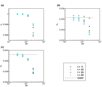
3.7 Results for Shear Layer B at different times and resolutions. Correlationr1 (a), the

real part of the mode, (b) and the imaginary part of the mode (c). Open symbols correspond to correlation withu0_{and filled symbols with}_v0 _{. . . .} ₃₄

3.8 Scatter plots foru0_{(left) and}_v0_{for Shear Layer A, ∆}_x_{= 0}_._{0625 and}_t_{= 20 . . . .} ₃₅

3.9 Scatter plots foru0_{(left) and}_v0_{for Shear Layer B, ∆}_x_{= 0}_._{0625 and}_t_{= 20 . . . .} ₃₅

3.10 Correlationr2(circles) as a function of the frequencyω for Shear Layer A (left) and B

at timet= 20. Also plotted is the dispersion relation (continuous line). This tests the value ofωwhere the maximum inr2occurs. The maxima of−αiandr2correspond to

the same valueω, therefore the correlation is maximum at the forcing frequency. The forcing frequency chosen corresponds to the maximum of−αi . . . 36

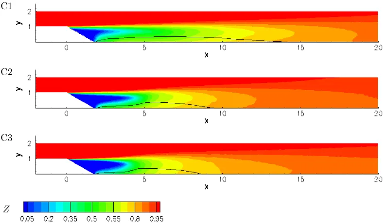
4.1 Computational domain configuration . . . 38 4.2 Instantaneous scalar iso-surfaces for Case C2. Iso-surfaces correspond toZ= 0.8 (red),

Z= 0.5 (green), andZ = 0.2 (blue). Notice the large spanwise-organized structures in the primary shear layer. . . 42 4.3 Instantaneous scalar contours on the mid span plane (top) and bottom wall for Case

C3. Black contour corresponds to the value of zero streamwise velocity. The flow is moving upstream in regions between the black contour and the lower wall or when surrounded by the black contour. The corresponding u-velocity field is shown in Fig. 4.4. . . 43 4.4 Instantaneous scalar contours on the mid span plane (top) and bottom wall for Case

(11)

4.5 Plane-averaged inflow and outflow pressure as a function of time for Case C2. Thin lines denote pressure averaged over planes normal to the streamwise direction near the inflow and outflow. Outflow pressure is always higher than the inflow. Thick lines are a rolling average of the pressure traces, with an averaging period of 3tc. . . 45 4.6 Change of the mean streamwise velocity profile for Case C2 with respect to the

stream-wise coordinate . . . 46 4.7 Contours of mean passive scalar and mean streamlines for Case C2 . . . 46 4.8 Mean scalar fields for Cases C1–3. Black contour corresponds to the value of zero

streamwise velocity. The flow is moving upstream in regions between the black contour and the lower wall. Case C1, the lowest resolution simulation, predicts a longer mean recirculation zone. . . 48 4.9 Mean profiles for Cases C1–3 at different streamwise locations, from left to rightx=4,

8, and 16. Blue dash-dot lines correspond to Case C1, lowest resolution; green dashed lines to Case C2, medium resolution; red solid lines to Case C3, highest resolution. . . 49 4.10 Turbulent kinetic energy (subgrid plus resolved) and ratio of turbulent kinetic energy

to subgrid turbulent kinetic energy for Cases C1–3 at different streamwise locations, from left to rightx=4, 8, and 16. Blue dashed-dot lines correspond to Case C1, lowest resolution; green dashed lines to Case C2, medium resolution; red solid lines to Case C3, highest resolution. . . 50 4.11 Minimum and maximum values of the passive scalar as a function of time for three

different resolutions. Blue lines correspond to Case C1, lowest resolution; green to Case C2, medium resolution; red to Case C3, highest resolution. . . 51 4.12 Volume fraction of the undershoots of the passive scalar as a function of time for

three different thresholds and resolutions. Blue lines correspond to Case C1, lowest resolution; green to Case C2, medium resolution; red to Case C3, highest resolution. . 52 4.13 Volume fraction of the overshoots of the passive scalar as a function of time for three

different thresholds and resolutions. Blue lines correspond to Case C1, lowest resolu-tion; green to Case C2, medium resoluresolu-tion; red to Case C3, highest resolution. . . 52 4.14 Shapes of the beta-function PDF for different values of the varianceZf02_{. All}

distribu-tions have the same mean ˜Z= 0.6. . . 54 4.15 Probability density functions of the scalar at x = 6 for Case C3 at two transverse

(12)

4.16 Probability density functions for Case C2 at different streamwise locations. Each panel shows PDFs along the transverse direction. Color contours correspond to the the total PDF whereas black contours to the resolved. Both contour sets have identical increments. 58 4.17 Scalar probability density functions for cases C1–3 at different streamwise locations.

Color contours correspond to the the total PDF whereas black contours to the resolved. Contours in all panels have identical increments. . . 59 4.18 Comparison of pressure coefficient along the lower (blue) and upper (red) guide walls.

Lines correspond to Case C2 of the simulations and circles to the experiments of John-son (2005). . . 60 4.19 Comparison of normalized temperature rise for H2rich (φ= 1/8) and F2 rich (φ= 8)

atx= 7.8 . . . 61 4.20 Probability of mixed fluid atx= 7.8 . . . 62 4.21 Instantaneous scalar fields for Cases D2 and E2 along mid span. Case E2, the lower

panel, has about twice the mass flux ratio of lower/upper stream resulting in different characteristics of the flow in the recirculation zone. Black contour corresponds to the stoichiometric mixture fraction for a notional octane (C8H18) fuel, Zst,C8H18 = 0.94,

ignoring heat-release effects. . . 64 4.22 Mean scalar fields for Cases D2 and E2. Black continuous contour corresponds to the

stoichiometric mixture fraction for a notional octane (C8H18) fuel, Zst,C8H18 = 0.94.

Dashed contour to the stoichiometric mixture fraction for a notional hydrogen (H2),

Zst,H2 = 0.97. The white contour near the lower wall corresponds to zero streamwise

velocity. . . 64 4.23 Schlieren visualization of the flow in the expansion ramp geometry from the experiments

of Johnson (2005). Upper streamU1≈120 m/s, lower steamUR≈5.5 m/s (left) and

UR≈12.5 m/s. . . 64

4.24 Total (resolved and subgrid) scalar probability density functions for Cases D2, low injection, (left column) and E2, high injection, at three streamwise locations. Contours are drawn at identical intervals in all panels. . . 66 4.25 The pressure coefficient on the lower and upper guide walls for Case D2. Symbols

correspond to a pair of experiments at the same conditions. . . 68 4.26 The pressure coefficient on the lower and upper guide walls for Case E2. Symbols

correspond to a pair of experiments at the same conditions. . . 68 4.27 Total pressure comparison for Cases D2 and E2 at x= 9.4. Symbols correspond to a

(13)

4.28 Normalized temperature rise and probability of mixed fluid for Case D2. Left column panels correspond to the upstream rake location, x = 7.2, and right column to the downstream rake location, x = 9.4. Experimental measurements are indicated by symbols. . . 70 4.29 Normalized temperature rise and probability of mixed fluid for Case E2. Left column

panels correspond to the upstream rake location, x = 7.2, and right column to the downstream rake location, x = 9.4. Experimental measurements are indicated by symbols. . . 71 4.30 Pressure coefficient at the exit of the test section, x= 7.2, as a function of the

mass-injection ratio. Open symbols correspond to the experiments of Johnson (2005) and Bergthorson et al. (2008), filled symbols to the present simulations (Cases C2, C3, D2 and E2). Continuous line is the control volume model of Bergthorson et al. (2008) (Eq. 4.34). . . 73 4.31 Computed streamwise velocity profiles atx= 7.2 . . . 73 4.32 Probability density functions at x = 8 for two resolutions, Case C3 has twice the

(14)

List of Tables

3.1 L1 convergence rates for the vortex test case . . . 21

3.2 Number of cells along each direction,N, and the corresponding approximate solutions attfinal . . . 25

3.3 Flow conditions for the two shear layers . . . 29 3.4 L2 norms of the linear and non-linear terms for the unconfined, incompressible Shear

Layer A . . . 31 3.5 L2 norms of the linear and non-linear terms for confined, compressible Shear Layer B 31

3.6 Comparison of the exact and computed real and imaginary parts of the most unstable mode for Shear Layer A foru0andv0. The grid resolution is 1600×640 (∆x= 0.0625). 33 3.7 Comparison of the exact and computed real and imaginary parts of the most unstable

mode for Shear Layer B foru0andv0. The grid resolution is 1600×640 (∆x= 0.0625). 34

4.1 Conditions for the cases simulated . . . 39 4.2 Ratio of grid spacing to the Kolmogorov,λK, and Liepmann-Taylor scale,λT . . . 47

4.3 Comparison of the difference between the experiments and the simulation for Cases C1–3. The values of the table correspond to the L1 distance between the data of

experiments and simulations normalized by theL1 norm of the experimental curves. . 63

4.4 Comparison of the difference between the experiments and the simulation for Cases D2 and E2 for two downstream locations. Upstream rake location is at x= 7.2 and downstream atx= 9.4. The values of the table correspond to theL1distance between

the data of experiments and simulations normalized by theL1norm of the experimental

(15)

Chapter 1

Introduction

Mixing on a molecular scale of two or more fluids of different composition is achieved by the action of diffusion. The rate of mixing of different species is of great importance because the speed of chemical reactions in many applications, such as fuel combustion, is limited by the availability of molecularly mixed reactants.

Diffusion is a relatively slow process because it relies on molecular collisions. Fortunately, (macroscopic) large-scale motions can significantly enhance the rate of mixing. Reynolds (1883) first introduced a dimensionless parameter, now called the Reynolds number, after observations of laminar-turbulent flow transition in a pipe. The Reynolds number, defined as

Re=U δ

ν , (1.1)

relates the characteristics of the aforementioned “large-scale motions” through the velocity of the fluid,U, and an appropriate length scale of the motion,δ, to the diffusion coefficient of momentum,

ν, also called the kinematic viscosity. Stability analysis of flows (e.g, Drazin & Reid, 2004) later corroborated the observation of Reynolds (1883) that when the Reynolds number is sufficiently large “. . . the flow rapidly becomes complicated and confused” as stated in (Landau & Lifshitz, 1959, p. 108), who continue to add that “Such flow is said to be turbulent,” thereby giving a rudimentary definition of turbulence.

(16)

1.1

Motivation—Enhanced mixing for air-breathing

propul-sion applications

Motivation for this work is the investigation of fundamental fluid dynamics important to the per-formance of combustors for hypersonic air-breathing propulsion applications, such as supersonic-combustor ramjets (scramjets) (Curran & Murthy, 2000; Curran, 2001). The foremost challenge in the design and operation of scramjet engines is addition of energy to a supersonic stream by mixing and combusting a fuel. Although this can be accomplished by a variety of passive and active mech-anisms, practical considerations require high combustion efficiency with reduced-length combustors (Curran et al., 1996; Seiner et al., 2001).

The two canonical flows most widely used in the study of turbulent mixing are jets and shear or mixing layers. Typical configurations for enhanced mixing in supersonic flow combustors rely on combinations of jets and shear layers (Gutmark et al., 1995; Kutschenreuter, 2000). Enhanced mixing alone is not sufficient. Regions of strain rate lower than the extinction strain rate of hydrocarbon fuels are required for sustaining combustion (Egolfopoulos et al., 1996) together with low total pressure losses to achieve the necessary propulsion efficiency.

In a shear or mixing layer, two near-parallel streams of unequal velocities, initially separated by a thin spitter plate, are allowed to mix. Many studies have investigated the characteristics of this flow in the context of turbulent mixing. Brown & Roshko (1974) noted the presence of large spanwise organized structures in incompressible, high-Reynolds-number shear layers. Konrad (1976) observed that after the transition of the flow from laminar to unsteady, due to the formation of the large coherent structures, another type of transition occurred further downstream of the splitter plate, that is, at a higher Reynolds number. This type of transition was associated with the ability of the flow to sustain three dimensional fluctuations with the appearance of smaller scales and streamwise vortices on the surface of the large structures. In similar observations in a chemically reacting shear layer Breidenthal (1978) showed that the onset of three dimensionality was correlated with a rapid transition (increase) in the amount of product, which he refers to as the “mixing transition.” The mixing transition in turbulent flows was later documented for other flows and introduced in a formal framework by Dimotakis (2000). Dimotakis (2000) notes that the mixing transition is a universal property of turbulence occurring when there is sufficient separation of scales to sustain fully developed turbulence.

(17)

process (Eckart, 1948). Using the shear layer as an example: the fluid is initially entrained in the mixing layer through the action of the large scale structures, is then stirred by turbulence and at the smallest space-time scales is homogenized by diffusion.

Mixing in compressible shear layers has not been as well characterized. The growth rate of the mixing zone, which sets an upper bound on the mixing, decreases with increasing compressibility (Papamoschou & Roshko, 1988; Slessor et al., 2000), however, contradictory trends are reported for the fraction of the mixed fluid in the mixing layer with respect to compressibility (Hall et al., 1991; Island et al., 1996; Freund et al., 2000; Rossmann et al., 2004). The reduction in growth rate and the amount of mixed fluid are both important issues in the context of air-breathing high-speed propulsion.

Jets in crossflow are another canonical flow that has been studied extensively (Zukoski & Spaid, 1964; Spaid & Zukoski, 1968; Hollo et al., 1994; Smith & Mungal, 1998; Ben-Yakar et al., 2006; Shan & Dimotakis, 2006). The jet in crossflow has higher entrainment rate than a jet into a quiescent reservoir, however, in supersonic flow, a bow shock forms upstream of the injector resulting in high total-pressure loses. The bow shock causes the boundary layer to separate, creating a flameholding region where fuel and air can mix subsonically (Zukoski & Spaid, 1964; Spaid & Zukoski, 1968; VanLerberghe et al., 2000). As a way of improving the flameholding characteristics of the device, a cavity can be added downstream of the injection (Yu et al., 1998; Ben-Yakar & Hanson, 2001; Yu et al., 2001) but with a significant drag penalty generated by the forward-facing facet.

1.2

The expansion-ramp injection geometry

Jets and shear layers alone cannot satisfy the performance requirements of supersonic combustors. Shear layers have negligible total pressure losses but the mixing is limited by the shear layer growth. Transverse and inclined jets, on the other hand, produce bow shocks that reduce the efficiency of the device.

In this work, the flow and mixing in an expansion-ramp geometry is studied through numerical simulations. The expansion-ramp geometry (Fig. 1.1) combines the low strain-rate flameholding characteristics of backward facing steps with low-pressure losses of free shear layers (Johnson, 2005; Bonanos et al., 2007, 2008a; Bergthorson et al., 2008; Bonanos et al., 2008b). In the expansion-ramp configuration the top, high-speed (“air”) stream is expanded over a ramp at 30◦ _{to the flow. The}

(18)

L

p

Probe location

Upper guidewall

Lower guidewall

α

h

U

1

U

_R

h

Figure 1.1: Schematic of the expansion-ramp geometry. The top stream,U1, enters the test section

in the horizontal direction while the lower stream, UR, is injected through a perforated ramp at

α= 30◦_{. The separating top stream forms the primary shear layer, which reattaches downstream}

(not pictured) with part of the flow being deflected upstream in the recirculation region. The upstream moving fluid forms a secondary shear layer where the ramp meets the lower guide wall.

layer curves toward the lower guide wall and reattaches.

Within the reattachment region on the lower wall, the shear layer splits with part of the flow deflected upstream into the recirculating flow region formed between the ramp and the reattachment (see Fig. 1.1). The deflection of the shear layer upstream is similar to the re-entrant jet formed at the end of a cavitation region (e.g., Callenaere et al., 2001). The re-entrant jet carries hot products and radicals upstream that mix with lower-stream fluid forming a secondary shear where the ramp meets the lower guide wall. This is a second mixing layer that allows products to further mix with the lower stream. The recirculating region, re-entrant jet, and the secondary shear layer allow for enhanced mixing compared to a free shear layer while providing a low strain-rate environment (Johnson, 2005; Bergthorson et al., 2008; Bonanos et al., 2008b).

The length of the recirculation zone can be controlled through variation of the mass-injection ratio of the two streams. Increasing the injection pushes reattachment downstream leading to a change in the pressure coefficient at a given streamwise location. Heat release via exothermic reaction in the shear layer has the same effect as increasing the mass flux of the lower stream because of the reduced volumetric entrainment of free-stream fluid (Hermanson & Dimotakis, 1989; Johnson, 2005; Bergthorson et al., 2008; Bonanos et al., 2008b).

1.2.1

Description of the experiments

(19)

measure-ments. A brief description of the experiments is presented here in order to facilitate the discussion of the comparison between experiments and simulations. Further details can be found in Johnson (2005), Bonanos et al. (2007), Bergthorson et al. (2008), Bonanos et al. (2008a), and Bonanos et al. (2008b).

The experiments were performed in the Supersonic Shear Layer (S3_{L) laboratory at Caltech (Hall}

et al., 1991). The top stream is delivered from a large pressure vessel using a control program to maintain constant pressure in the upstream plenum and can reach flow speeds up toM1≈3.2. The

lower stream has a constant mass flux, metered using a calibrated sonic valve. The two streams are accelerated through converging nozzles designed to minimize the boundary-layer thickness on the splitter plate and turbulence generation at the design Mach number. The lower stream is injected through a perforated expansion ramp angled atα= 30◦ with respect to the horizontal. The ramp is perforated with 3611 1.55-mm-diameter holes, corresponding to an open-area fraction of 0.60. The test section height is 2h= 10.16 cm, with the individual stream height beingh(Fig. 1.1). The nominal run time in the facility is 2–6 seconds.

The H2/NO/F2system is used to study the mixing in the expansion ramp geometry. Specifically,

the top stream is seeded with a mixture of hydrogen (H2) and nitric oxide (NO), and the bottom

stream with fluorine (F2). The remainder of the gas in both streams is comprised of helium, argon,

and nitrogen inert diluents, with compositions chosen to match the molar mass and specific-heat ratio of the two streams. Nitric oxide is added to the hydrogen stream to generate radicals on contact with fluorine to initiate the hydrogen-fluorine reaction (Mungal & Dimotakis, 1984). The reaction then proceeds without an ignition source (hypergolically) at room temperature.

Flow-field measurements are obtained by pressure taps along the lower and upper guide walls, and a measurement rake that can be placed at distances Lp = 7h– 9hdownstream of the splitter

plate. Temperature and total and static pressures are measured at the rake through an array of thermocouple and pressure probes. In addition to temperature and pressure data, Schlieren flow visualization is utilized as a concurrent non-intrusive diagnostic. Figures 1.2 and 1.3 show Schlieren images of the flow for two mass-injection ratios (Johnson, 2005). The primary and secondary shear layers are clearly visible in Fig. 1.2. In Fig. 1.3 the increased injection pushes the recirculation zone downstream. The upstream-moving mixed fluid does not reach the ramp to form the secondary mixing layer and the flow becomes similar to a free shear layer.

(20)

Figure 1.2: Schlieren visualization of the flow in the expansion ramp geometry from the experiments of Johnson (2005). The primary and secondary shear layers are clearly visible. Upper stream

U1 ≈120 m/s, lower steam UR ≈5.5 m/s. Upper stream composition is N2 and lower stream is

66.66% Ar, 33.33% He (non-reacting flow).

Figure 1.3: Schlieren visualization of the flow in the expansion ramp geometry from the experiments of Johnson (2005). Upper streamU1 ≈120 m/s, lower steamUR≈12.5 m/s. Upper stream

compo-sition is N2 and lower stream is 66.66% Ar, 33.33% He (non-reacting flow). The increased injection

(21)

limitations in spatial resolution since only fluid mixed on a molecular scale reacts and contributes to the temperature rise.

The “flip” experiment relies on two underlying assumptions: that the experiments are performed in the mixing-limited regime and that the flow in the pair of experiments remains unchanged with the changing location of the temperature rise. The first assumption is validated by computing the Damk¨ohler number,Da≡τm/τχ, the ratio of the mixing time scale to the chemical time scale for

experiments that have converged with respect to chemical reaction rates. The chemical time scale is estimated using the “balloon-reactor” model of Dimotakis & Hall (1987). The studies of Hall et al. (1991), Slessor et al. (1998), and Bond (1999) have shown that the flow is mixing-limited when

Da > 1.5. In the experiments considered here, this condition is satisfied. The assumption that the flow must remain unchanged in the pair of experiments is assessed by examining the stagnation pressure profiles recorded along the measurement rake (Johnson, 2005; Bergthorson et al., 2008; Bonanos et al., 2008b). The flow is deemed matched if the stagnation pressure profiles are in agreement.

1.3

Modeling for turbulent mixing and nonpremixed

com-bustion

The objective of this study is the numerical simulation of the flow in the expansion-ramp geometry corresponding to subsonic experimental conditions. The experiments documented in Johnson (2005) and Bergthorson et al. (2008) provide good information on the flow field and mixing characteristics for a range of conditions and a well-documented, suitable arena against which to validate numerical simulations.

The main goal of the current work is to address the prediction challenge in the computational simulation of complex flows. The experiments in the expansion-ramp geometry provide a framework for the assessment of such models for turbulent momentum and species mixing. Although the current work is concerned with a specific numerical model, the assessment methodology is generally applicable and the outcome provides guidance for further development.

The numerical model is now characterized in more detail. Numerical integration of the Navier– Stokes equations provides the evolution of the fluid mechanical fields. However, the broad range of spatial and temporal scales characterizing most turbulent flows of interest place direct numerical simulation (DNS) beyond practical reach. Several methods have been developed to obtain approx-imate solutions that capture the behavior of turbulent flows. Such methods are called turbulence models.

(22)

only a small fraction of the turbulent kinetic energy, are more homogeneous and universal, and typically are less sensitive to modeling assumptions (Tennekes & Lumley, 1972; Pullin, 2000; Pope, 2004a). In the simulations presented here, LES with subgrid scale modeling (LES–SGS) is employed, where the effects of scales smaller than those resolved by the simulation are explicitly described by the turbulence model as opposed to relying on the dissipation supplied by the numerical scheme used to approximate the spatial derivatives.

LES is a widely used technique for the simulation of turbulent flows and a number of reviews have addressed this approach (e.g., Lesieur & Metais, 1996; Ghosal, 1999; Piomelli, 1999; Meneveau & Katz, 2000; Oefelein, 2006; Pitsch, 2006). The LES equations are derived from the Navier–Stokes equations by performing a filtering operation (Leonard, 1974) with a filter width usually of the size of the grid spacing. The filtering produces additional terms, a tensor in the momentum equations and fluxes for the energy and species equations. The subgrid-stress tensor and energy and species fluxes, cannot be expressed solely as functions of the filtered quantities and must be modeled.

LES has been successful in the simulation of many non-reacting flows (Lesieur & Metais, 1996) but the simulation of turbulent mixing in reacting and non-reacting flows still presents many challenges. See, for example, Peters (2000) and Poinsot & Veynante (2005). Turbulence models for momentum transport rely on theoretical advances like the eddy cascade and scale invariance in the inertial subrange (Tennekes & Lumley, 1972; Pope, 2004a). On the other hand, mixing on a molecular scale takes place only at the smallest scales of the flow (Dimotakis, 1991, 2005; Warhaft, 2000). Most of the fluid homogenization occurs subgrid, and SGS models must “infer” subgrid mixing based on the resolved scales. Turbulent mixing in reacting flows presents additional challenges since mixing produces changes in the composition of the fluid which can change the dynamics of the flow.

The subgrid terms are often modeled using the gradient-transport assumption in the context of Smagorinsky-type models (Smagorinsky, 1963). For such models, the SGS stress tensor takes the form

τij =−2 ¯ρ Cs∆2|Se|S,e (1.2)

and the subgrid scalar flux (Moin et al., 1991)

gi=−ρ¯

whereSeis the resolved (filtered) strain tensor, ∆ is the filter width,ρis the density andZ the scalar concentration. Closure is attained by introducing the concept of turbulent Prandtl number,P rtin

combination with the Smagorinsky coefficient,Cs. The SGS momentum transport can be expressed,

similar to the SGS scalar flux, in terms of a turbulent viscosity coefficient,νt. These formulations are

(23)

(Moin et al., 1991) and, for some flows, assuming constant values throughout the flow produces overly dissipative models (Ducros et al., 1996).

Germano et al. (1991) suggested a dynamic procedure for the estimation of the Smagorinsky coefficient by introducing a test filter ˆ∆ in addition to the grid filter ∆. The width of the test filter is usually set to twice the grid filter. Moin et al. (1991) implemented the Dynamic Procedure to estimate the turbulent Prandtl number in Eq. 1.3.

Pullin et al. (Pullin & Saffman, 1994; Misra & Pullin, 1997; Voelkl et al., 2000; Pullin, 2000) proposed a vortex-based model for the SGS stresses and fluxes based on the exact Navier–Stokes solution by Lundgren (1982) for a vortex in a strain-rate field. In this model the subgrid fields are represented by a collection of vortical structures. The resulting expression for the subgrid tensor depends on the energy spectrum of the vortex,E(k), and the distribution of the orientation of the vortical structures,

τij= 2

Z ∞

π/∆

E(k)dkhEpiZpqEqji. (1.4)

Epi is the transformation matrix from the vortex-fixed to the laboratory frame of reference, Zpq is a diagonal matrix with the elements (1/2, 1/2, 0), and hEpiZpqEqji signifies the ensemble average over the orientations of the vortex structures.

In the case of subgrid scalar transport, the SGS flux is estimated by assuming that the scalar is wrapped by the SGS vortex velocity field, resulting in a tensor eddy-diffusivity model for SGS transport. The subgrid transport is not in the direction of the resolved gradient but orthogonal to the subgrid vorticity (Pullin, 2000; Pullin & Lundgren, 2001).

The basis for most nonpremixed combustion models is to track the mixing of fuel and oxidizer by a passive scalar. If the chemistry is fast enough (high Da) a reaction layer forms at approx-imately stoichiometric composition and the flame can be assumed to have a negligible thickness (Burke & Schumann, 1928). This is true for high activation energy reactions, such as combustion of hydrocarbon fuels, but is not the case for the H2/NO/F2 system. For infinitely fast chemistry, all

species mass fractions and temperature can be expressed as function of a passive scalarZ. When parameterizing the combustion by the passive scalarZ, the effects of chemical reactions and heat release are entirely neglected. Akselvoll & Moin (1996) and Pierce & Moin (1998) conducted LES of passive scalar mixing of turbulent confined coannular jets using the gradient-transport model (Eq. 1.3) employing the Dynamic Procedure (Germano et al., 1991; Moin et al., 1991).

(24)

Klimenko (1990) and Bilger (1993) independently introduced the concept of conditional moment closure (CMC); see also Klimenko & Bilger (1999) for a more recent review. Unlike the flamelet models, in CMC one solves the equations for reactive scalars conditioned on the mixture fraction

Z. This can be advantageous from the modeling perspective and computationally more efficient (Klimenko, 1990), however, it adds more independent variables to the equations, namely the scalar(s)

Zi.

Another class of models is based on probability density function (PDF) transport equations. Pope (1990) proposed the use of the equation for the joint PDF of velocity, viscous dissipation and reactive scalars, corresponding to single realization of the subgrid state of the mixture. Gao & O’Brien (1993) and Colucci et al. (1998) also studied and extended the PDF transport method while Hulek & Lindstedt (1998) used a joint scalar-velocity formulation in simulations of mixing with chemical reactions in a scalar mixing layer in grid turbulence. Because of the high dimensionality of the PDF transport equations, numerical implementations typically rely on Monte-Carlo methods employing a large number of notional particles (Pope, 1985), resulting in high computational costs. Linear-eddy models (LEM) were first introduced by Kerstein (1988, 1989, 1990) and model SGS mixing using a one-dimensional stochastic approach. An extension of the ideas of the LEM to the velocity field by Kerstein (1999) is called the one-dimensional turbulence (ODT) model.

More recently, Pantano & Sarkar (2001) and Mellado et al. (2003) introduced a class of re-construction moments by combining an approximate rere-construction with additional physics-based information required to match specific scalar moments—the subgrid variance, for example.

(25)

Chapter 2

Numerical Modeling

2.1

Governing equations

The governing equations, in the context of large-eddy simulation, are the two-component Favre-filtered (density weighted) compressible Navier–Stokes equations. The Favre-Favre-filtered quantities are defined as

˜

f ≡ ρf ¯

ρ, (2.1)

for an arbitrary fieldf, where ρis the density. The overbar indicates the filtering operation

¯

f(x, t)≡ Z

G(x−x0)f(x0, t)dx0, (2.2)

with a convolution kernelG(x) (Leonard, 1974).

The mixing in the expansion-ramp geometry is parameterized in terms of the mixture fraction

Z. In the experiments, the rate of the chemical reactions is fast and the heat release is low. The adiabatic flame temperature rise is about 94 K for a mixture of 1% H2 in the upper stream and

1% F2 in the lower stream, both diluted with N2 (Johnson, 2005), resulting in an essentially cold

reaction. Therefore the passive scalar approximation is an adequate representation of reality. The mixing problem reduces to the mixing of a chemistry-independent conserved scalar Z, and most quantities of interest can be expressed as functions ofZ (see also, Williams, 1985; Peters, 2000).

The conservation equations for mass, momentum, energy and a passive scalar are, respectively,

∂ρ¯

∂t + ∂ρ¯u˜i

∂xi

= 0, (2.3)

∂ρ¯u˜i

∂t +

∂( ¯ρu˜ju˜i+ ¯pδij)

∂xj

= ∂σ¯ij

∂xj −∂τij

∂xj

(26)

∂E

The subgrid terms, τij, qi, and gi, represent the subgrid stress tensor, and the heat and scalar transport flux, respectively. The filtered total energy per unit volume,E, is the sum of the internal and kinetic energy (resolved and subgrid),

E= p¯

where the filtered pressure, ¯p, is determined from the ideal-gas equation of state,

¯

p= ¯ρRT .˜ (2.8)

Since the fully resolved fields are not available in LES, the filtering operation (Eq. 2.1) is purely formal, and only used to construct the LES equations. The subgrid terms cannot be evaluated using information derived from the resolved scales (closure problem) and a model, or additional information, are required to approximate them. Integration of the LES equations will yield the time evolution of the resolved fields. Any instantaneous realization of the resolved field carries limited information however, not only because of the characteristics of the modeling, but also because of the random nature of the turbulent flow. Therefore, one is primarily interested in the statistics of the resolved field and, through the use of models for the unresolved field structure, in pointwise quantities, such as the amount of mixed fluid on a molecular scale. A discussion on the conceptual foundations of LES can be found in Pope (2004b).

2.2

Subgrid closure

(27)

The expressions for the subgrid tensor and fluxes are

the subgrid cutoff scale, here taken to be equal to the grid spacing ∆x. The largest resolved wave number is thenkc =π/∆c. The energy spectrum for the Lundgren spiral vortex is

E(k) =K02/3k−5/3exp[−2k2ν/(3|α˜|)], (2.13)

whereK0is the Kolomogorov prefactor,is the local cell-averaged dissipation rate, and

|α˜|= ˜Sijevie v

j (2.14)

is the axial strain along the subgrid vortex axis.

˜

is the resolved rate-of-strain tensor. The factorK02/3 is estimated from the local, resolved-scale,

second-order velocity structure function ˜F2(r;x) (Metais & Lesieur, 1992; Voelkl et al., 2000),

K02/3=

A local spherical average is used to estimate ˜F2,

(28)

is the velocity difference of component ui in direction xj at x. This allows the SGS terms to be estimated dynamically only from the local instantaneous resolved fields without performing any temporal or spatial averages.

The SGS scalar mixing model, which is of particular interest here, is based on an analytical solution of the Navier–Stokes equations for the winding of the scalar field by the subgrid vortex (Lundgren, 1982; Pullin, 2000; Pullin & Lundgren, 2001). The anisotropic SGS mixing of the scalar by the vortex results in a tensor eddy-diffusivity model for the SGS scalar flux (Eq. 2.11). In LES of isotropic turbulence with an imposed mean scalar gradient, Pullin (2000) predicted the expected behavior for the normalized scalar variance as a function of the Taylor Reynolds number (Dimotakis, 2000). The model has also been applied to two-fluid mixing in Rayleigh–Taylor (Mattner et al., 2004) and Richtmyer–Meshkov (Hill et al., 2006) instabilities.

2.3

Numerical method

The numerical method is discussed in detail in Hill & Pullin (2004) and Pantano et al. (2007). The main features of the numerical method will be summarized here. The conservation equations are discretized on a regular Cartesian mesh using the second-order accurate, collocated tuned center-difference (TCD) scheme of Hill & Pullin (2004). The center-center-difference scheme uses a bandwidth-optimized five-point stencil constructed to minimize the spatial truncation error for the Navier– Stokes equations for a von K´arm´an spectrum (Ghosal, 1996, 1999).

The hybrid method of Hill & Pullin (2004) was developed for the simulation of flows with discon-tinuities, such as shock waves, and can switch to an upwinding weighted essentially non-oscillatory (WENO) scheme (Liu et al., 1994) from the centered differences in a cell-based fashion. In this study, all flows simulated were subsonic and WENO was not used in any part of the flow domain.

Both the finite differences and WENO are implemented with conservative flux-based discretiza-tions (Rai, 1986) and formulated in energy-conserving form (Zang, 1991; Honein & Moin, 2004), with stable boundary closures (Strand, 1994). Inflow and outflow boundary conditions on planes aligned with the grid are implemented in characteristic form, as suggested by Thompson (1987) and Poinsot & Lele (1992). A third-order strong stability preserving (SSP) Runge–Kutta method (Gottlieb et al., 2001) is used for time stepping.

2.4

Implicit geometry representation

(29)

the boundary of the physical domain,∂Ωf. The level-set function is defined as the signed distance

from the boundary∂Ωf. The computational cells are divided into two groups, depending on the sign

of the distance functionφ(xi, yj, zk) at the center of each cell, with the physical cells (fluid domain, Ωf) having positive distance from the boundary and ghost cells at negative distance (ghost fluid

domain, Ωg).

The vector of state in the ghost cells is not part of the solution, and can even assume non-physical values. The thin layer of ghost cells adjacent to the boundary is used to apply the desired boundary condition on∂Ωf. This method of applying the boundary condition was first introduced by Fedkiw

et al. (1999) and is known as the ghost fluid method (GFM). The band of cells that are modified in the ghost fluid is chosen to be wide enough to ensure that stencils centered on cells in the physical domain will not reach beyond this band of ghost cells, for the simulations in the current study are three cells deep in each direction in order to accommodate calculation of quantities used by the LES model.

The GFM method allows the governing equations to be solved on a Cartesian mesh without the need to generate boundary-conforming grids. The solution in the entire computational domain, physical and ghost fluid, is updated by the solver at each time step, thus avoiding the stability con-straints associated with the generation of arbitrary small “cut cells” where the boundary intersects the regular Cartesian grid. Moreover, computational complexity is reduced since ghost fluid cells require no special treatment by the integration algorithm.

2.4.1

No-penetration boundary condition—Slip wall

For the current simulations, two types of boundary conditions have to be imposed: a no-penetration condition on solid walls (slip wall) and an inflow condition for the injection ramp. The linear extrapolation or mirroring described in Arienti et al. (2003) is used to populate the ghost cells in the case of the no-penetration condition. The goal here is to construct ghost-cell states such that the interpolated normal component to the boundary velocity component is zero. For each ghost cell at

xg the mirror imagexg0 is found and then the vector of stateU(x_g0) is interpolated atx_g0 from the neighboring cells in the physical domain (Fig. 2.1). The valueU(xg) is then computed by inverting

the sign of the normal velocity component ofU(xg0) with respect to∂Ω_f.

2.4.2

Subsonic-inflow boundary condition

(30)

∂ Ω _f Ω _f

Ω g

x_g

x_g’

Cell in the physical domain Cell in the ghost fluid domain

Ghost cell used in the application of boundary condition Mirror points corresponding to ghost cells

Figure 2.1: Schematic showing a two-dimensional computational grid intersected by a level set defined boundary, ∂Ωf (thicker line). The grid is divided in two regions, the physical domain (Ωf)

and the ghost fluid (Ωg). Filled black circles denote the band of cells adjacent to the boundary that

have to be populated by the ghost fluid method, assuming here that the width of the stencil is 5 cells. The mirror points,xg0, ofx_g, with respect to the boundary, are also shown (squares) for some of the ghost cells.

to time) of the overall discrete method. A method akin to the ones used for finite-volume schemes (Wesseling, 2001) was chosen to fill the ghost cells that accounts for the outgoing characteristic.

The number of “Euler” boundary conditions that must be prescribed at a subsonic inflow bound-ary is equal to the number of the incoming characteristics, that is, four in three-dimensional flow. In the experiments, the mass flux through the ramp is fixed by the flow through a sonic valve sup-plying an upstream plenum. Therefore the density and the velocity vector in the ghost cells are set to constant values corresponding to the set mass flux of the lower stream. An extrapolation along the outgoing characteristic is carried out to completely determine the vector of state in the ghost cells.

(31)

The conservative-variables vector of state

U= [ρ, ρu1, ρu2, ρu3, E, ρZ]T (2.20)

must be prescribed inside the ghost fluid. Setting the density and the velocity vector to constant values corresponding to the mass flux through the ramp leaves the total energy,E, to be computed by extrapolation along the outgoing invariant. For the calculation of the total energy in the ghost cells, first the outgoing Riemann invariant is considered,

R5=u+

2

γ−1c, (2.21)

wherec is the speed of sound anduis the velocity component normal to the inflow boundary. The speed of sound in the ghost cell is

cg=

which is used to compute the unknown total energy

Eg=ρg

wherev andware the two tangential to the boundary components of the velocity vector.

Due to the continuous update of the ghost fluid cells adjacent to the boundary, so that the boundary condition on the boundary is satisfied at the beginning of each time step, the flow in the interior ghost fluid can be quite severe and even unphysical. Nevertheless, the integration algorithm does not distinguish between the physical fluid and the ghost fluid, therefore, in order to avoid a breakdown or “blowup” of the integration, the dissipative WENO scheme is used to advance the solution (only) in the ghost fluid.

Although integrating the entire domain has many advantages from an algorithmic point of view, it may negatively affect the performance of the overall simulation by restricting the time step in the case of some unusual flow feature developing in the ghost fluid region. In this work, there is no evidence that the time step is restricted by the ghost fluid, possibly because the geometry of the simulation domain is not particularly complex.

2.5

Implementation framework

(32)

(33)

Chapter 3

Verification

The American Institute of Aeronautics and Astronautics defines verification as follows (AIAA, 1998):

Definition 1 (Verification) The process of determining that a model implementation accurately represents the developer’s conceptual description of the model and the solution to the model.

The model in the case of computational fluid dynamics is, typically, a set of differential equations with the corresponding boundary conditions. Computational simulation seeks solutions to the conceptual model by converting the continuum equation(s) to a discrete model and then applying a suitable computational algorithm. Verification provides substantiation that the technique of computing the solution is correct. Since the method of acquiring numerical solutions is comprised of a mathematics part, discretizing the continuum equations, and a computer-science part, implementing (that is programming) a suitable algorithm, verification has two fundamental aspects: solution verification and code verification. In this work, the distinction is not made between the two since all the verification techniques applied test both the discretization and the computer program.

From the definition of the verification process, it is evident that the model is not required to de-scribe any real-world physics. The assessment of the accuracy of a model in predicting experimental data is undertaken by the validation process. The definition of validation according to AIAA (1998) is given here for completeness:

Definition 2 (Validation) The process of determining the degree to which a model is an accurate representation of the real world from the perspective of the intended uses of the model.

Model validation will be discussed in the next chapter.

(34)

in computer performance there has been a similar growth in program size and complexity (Post & Votta, 2005), which makes the challenge of verifying a code with tens or hundreds of thousands of lines in which multi-physics models are involved considerable (Hatton, 1997).

Verification techniques in computational fluid dynamics can rely on grid convergence, order of accuracy, Richardson extrapolation, and comparison to benchmark solutions. Numerical results can also be compared against known analytical solutions or against fictitious manufactured solutions (Knupp & Salari, 2003; Steinberg & Roache, 1985). A number of reviews have compiled these and other techniques to assess program code accuracy (Knupp & Salari, 2003; Oberkampf & Trucano, 2002; Roache, 1998; Roy, 2005).

In the simulations of the reattaching shear layer, the unsteady, compressible, filtered Navier– Stokes equations are integrated numerically. Verification of the solver would require using a viscous flow as a test case. However, in the high Reynolds number flows of interest, the viscous terms are much smaller than the convective and subgrid terms and will be neglected for the purposes of verifying the solver.

Our experience has showed that, because of their lack of dissipation terms, the Euler equations are a very good test for verification purposes. In the turbulence simulations considered, the LES model has a stabilizing action on the under-resolved flow and can also act to stabilize mild instabilities that may be produced by the numerical scheme. Therefore, although the Euler equations are missing some of the physics of the Navier–Stokes equations, they constitute a strict test for the numerical scheme.

3.1

Exact solution of the Euler equations using periodic

bound-ary conditions

The simple two-dimensional vortical solution of the Euler equations with periodic boundary condi-tions in both dimensions employed by Balsara & Shu (2000) was used to study the convergence of the interior stencil. The tangential velocity distribution is

uθ(r) =rexp(−r2), (3.1)

where ris the radial coordinate from the center of the vortex. Assuming a perfect gas equation of state, from the radial momentum equation the pressure distribution is

p(r) =p0

1−γ−1 γ

ρ0

4p0

exp(−2r2)

γ γ−1

(35)

where, p0 and ρ0 are the free-stream pressure and density respectively. The density is computed

from the pressure and the free-stream state,p/ργ ₌_p

0/ρ

γ

0. For the test presented hereρ0= 1 and

p0= 2.

A passive scalar distribution of the form

Z(r) = exp(−r2), (3.3)

is superimposed on the velocity field in order to assess the solution of the passive scalar transport equation.

The flow is computed on a grid of [−5,5]×[−5,5] units. The vortex radius is about one unit. The computation is initialized with Eqs. 3.1, 3.2 and 3.3 and computed to timet/tr= 1 using the

second-order-accurate tuned-centered-difference (TCD) stencil. tr is the time of a single revolution

of the vortex and is defined as

tr= 2πr/uθ(r), (3.4)

withr= 1.

Convergence is assessed by computing the L∞ and L1 norms of the error att/tr= 1 for mass,

momentum, total energy and, mixture fraction for four grid resolutions. Because the solution and discretization are symmetric in the x and y directions, errors inxand y momentum are identical and a distinction between the two is not made here. The grid was refined by a factor of 2 in each dimension, starting with a coarse grid of 128 cells and leading to a finest at 1024 cells, in each direction.

The expected second-order convergence is observed for all quantities as can be seen in Fig. 3.1 and Table 3.1.

Mass Momentum Energy Mixture fraction

N Log Error Rate Log Error Rate Log Error Rate Log Error Rate

128 -5.73 -4.38 -3.77 -3.73

256 -7.21 2.14 -5.74 1.96 -5.24 2.11 -5.10 1.98

512 -8.61 2.02 -7.12 1.99 -6.64 2.02 -6.50 2.02

1024 -10.00 2.00 -8.51 2.00 -8.03 2.00 -7.88 1.99

Table 3.1:L1convergence rates for the vortex test case

The velocity distribution of the vortex is unstable to axisymmetric disturbances. The Rayleigh discriminant (e.g., Drazin & Reid, 2004) defined by

Φ(r) = 1

r3

d dr(r

(36)

∆x

Figure 3.1: L1 and L∞ norm of the error versus grid spacing for mass, momentum, energy, and

mixture fraction for the vortex test case with periodic boundary conditions

t / t_r

Figure 3.2: L1 norm of the density error versus time for a grid resolution of 256×256. A unit of

(37)

where Ω(r) = exp(−r2_{) is the angular velocity distribution of the vortex, is negative for} _{r >}_{1. A}

necessary and sufficient condition for stability to axisymmetric disturbances is that the square of the circulation does not decrease anywhere, that is, Φ≥0.

Although the initial condition has no perturbations, the accumulation of numerical error after sufficient time causes the flow to become unstable and the numerical integration eventually fails. Figure 3.2 shows the L1 norm of the error in density with respect to time. At the resolution of

256×256 it takes about 60 revolutions of the vortex before the instability develops. The norms in the convergence study were computed after one revolution, well before the instability develops.

3.2

Verification of the passive scalar diffusion term

imple-mentation

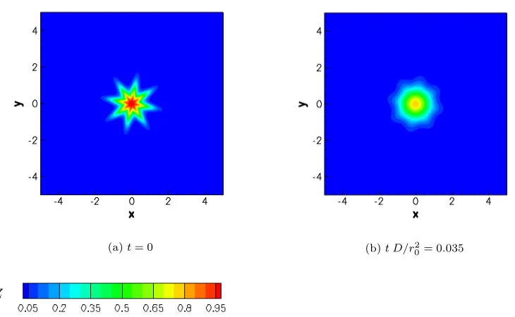
In order to verify the implementation of the diffusion term in the passive scalar equation, a two-dimensional diffusion problem for the scalar is considered. The initial condition has a scalar concen-tration in polar coordinates (r, θ),

Z(r, θ, t= 0) = exp[−(sin 8θ+ 2)(r/r0)2], (3.6)

with r0 = 1. The velocity vector is set to zero and the density and pressure are uniform. The

equations of motion and the equation for the scalar are integrated up to a time oftfinalD/r20= 0.035,

where D is the diffusion coefficient of the passive scalar. The initial and final concentration fields are shown in Fig. 3.3.

Since there is no exact solution for the evolution of Z(x, y, t) the observed order of accuracy is calculated following Roy (2005). The method for calculating the observed order of accuracy is similar to Richardson extrapolation (Richardson, 1910, 1927), however, unlike Richardson extrapolation, the order of accuracy of the scheme does not need to be assumed.

Consider three grids with uniform grid spacing ∆x1, ∆x2, and ∆x3, having a constant refinement

factor,h >1,

h= ∆x2 ∆x1

= ∆x3 ∆x2

, (3.7)

or

∆x1= ∆x, ∆x2=h∆x, ∆x3=h2∆x. (3.8)

If the solution ofZ(x, y, t) at tfinal is accurate to order p, then the solutions on the three grids can

(38)

(a)t= 0 (b)t D/r2 0= 0.035

Z

Figure 3.3: Initial condition for the passive scalar diffusion test case (left) and the scalar distribution at the end of the integration

spacing, ∆x:

Z1(x, y, tfinal) =Zexact(x, y, tfinal) +gp(x, y, tfinal)∆xp+O ∆xp+1

(3.9)

Z2(x, y, tfinal) =Zexact(x, y, tfinal) +gp(x, y, tfinal)(h∆x)p+O [h∆x]p+1

(3.10)

Z3(x, y, tfinal) =Zexact(x, y, tfinal) +gp(x, y, tfinal)(h2∆x)p+O [h2∆x]p+1. (3.11)

Neglecting higher-order terms and solving in terms ofp, yields the observed order of accuracy,

p=

lnZ3−Z2

Z2−Z1

ln(h) . (3.12)

The diffusion problem for the scalar was computed for four grid resolutions having h = 2 as shown in Table 3.2. Because the expressions for the error in Eqs. 3.9–3.11 are asymptotic with respect to ∆x → 0, relatively fine grids were used to compute the solution. The computational domain has a size of [−5,5]×[−5,5] units.

(39)

N Solution

256 Z4(x, y, tfinal)

512 Z3(x, y, tfinal)

1024 Z2(x, y, tfinal)

2048 Z1(x, y, tfinal)

Table 3.2: Number of cells along each direction,N, and the corresponding approximate solutions at

tfinal

The observed order of accuracy agrees with the order of accuracy of the scheme.

3.3

Assessment of the solver using correlations with linear

stability analysis

The vortical flow considered in Section 3.1 is sufficient to establish convergence of the interior scheme, however, it is rather simple and non-representative of the turbulent shear flow and, more importantly, does not assess the performance of the boundary closure. For this reason, an unsteady and spatially developing flow is used to assess those aspects of the code.

(40)

Dimotakis (2001) performed a comparison with a Navier–Stokes solver that includes the non-linear terms.

In the present study, the LSA solution for a spatially developing shear layer is used because of the simplicity of the basic flow and the similarity to the turbulent shear flow of interest. Spatially devel-oping, inviscid, compressible shear layers are computed using the present computational framework. The flow is forced at the inflow using the eigenfunctions and the corresponding frequency of the most unstable mode as computed from LSA. This is a common way for providing initial/boundary conditions or perturbations to shear flows (e.g., Colonius et al., 1997).

Direct comparison of the numerically computed solution with the LSA result presents many challenges. There are many reasons why the computed solution from an Euler solver may differ from the LSA solution. Solution of the boundary value (LSA) and the initial value (Euler solver) problem may not yield the same result, differences can be due to limitations of the boundary conditions, as a consequence of the practical difficulties associated with comparing an exponentially growing field, or because of differences in the basic flow.

Since the goal of comparison between the LSA prediction and the solution from an Euler solver is to assess computer code accuracy, a detailed listing and analysis of the reasons leading to differ-ences of the two solutions becomes of limited importance. LSA can be used to compute unstable perturbations to a flow, which are then used to force the flow computed by the solver been assessed. Therefore, the question posed here is different than determining whether a numerical solution converges to an analytical exact solution of the equations. That is, instead of attempting to obtain a hard measurement of the numerical error, one can attempt to determine how close the numerical solution is to the expected prediction from LSA. The value of such a metric, however, can be lower than that provided by convergence and accuracy tests since a solution that appears to be approaching an exact solution may ultimately not even be a mathematically consistent one. As a complement to traditional error metrics, one can exploit statistical metrics.

The closeness of the solutions can be measured in a number of ways, through projection techniques (Powell, 1981) to two-point correlations (Goldberg, 1960; McDonald, 1985). For the purpose of solver assessment, correlations can be used in a manner akin to that of identification techniques in image processing where geometrical shapes are identified by correlating an image against all possible sizes, orientations and positions of the corresponding primitive (e.g., Partridge, 1991).

3.3.1

Linear stability solution

(41)

Drazin & Davey (1977) assumed that the thermodynamic state of the flow is constant. Discussion of a secondary instability in three-dimensional shear layers appearing as streamwise counter-rotating vortices can be found in Metcalfe et al. (1987). In this work, the LSA solution for inviscid compress-ible free and confined spatial shear layers by Zhuang et al. (1990a,b) is utilized. Their method for deriving the stability characteristics for compressible spatial shear layers is summarized here. The reader is referred to Zhuang et al. (1990a,b) for details on deriving the stability characteristics and to Matheou et al. (2008) for the use of the present LSA solution for verification.

Consider a two-dimensional flow of two parallel steams. All quantities can be written as a basic profile ¯Q(y) plus a perturbation:

Q(x, y, t) = ¯Q(y) +Q0(x, y, t). (3.19)

Disturbance quantities denoted by primes can be written as an eigenmode expansion,

Q0=f(y) exp[i(αx−ωt)]. (3.20)

For spatially growing fluctuations, like the ones considered here,ωis a real frequency andα=αr+i αi

a complex wave number. The corresponding complex wave velocity can then be written asc=ω/α. Substituting the expressions for the disturbance quantities into the compressible Euler equations and neglecting quadratic and higher-order terms yields a system of ordinary differential equations for the amplitude functions. These equations can be reduced to a single equation for the pressure disturbances.

For a given disturbance frequency,ω, and a basic flow, the solution of the boundary-value problem for the pressure eigenfunction gives the complex eigenvalue,α. The eigenfunctions for the velocity and density can then be expressed as functions of the pressure eigenfunction and