Visual attention and object categorization: from psychophysics to computational models

Visual attention and object categorization:

from psychophysics to computational models

Robert J. Peters

In partial fulfillment of the requirements

for the degree of

Doctor of Philosophy

in

Computation and Neural Systems

California Institute of Technology

Pasadena, California

2004

Abstract

This thesis is arranged in two main parts. Each part relies an approach using the methods of psychophysics and computational modeling to bring abstract or high-level theories of vision closer to a concrete neurobiological foundation.

The first part addresses the topic of visual object categorization. Previous stud-ies using high-level models categorization have left unresolved issues of neurobi-ological relevance, including how features are extracted from the image and the role played by memory capacity in categorization performance. We compared the ability of a comprehensive set of models to match the categorization perfor-mance of human observers while explicitly accounting for the models’ numbers of free parameters. The most successful models did not require a large memory capacity, suggesting that a sparse, abstracted representation of category properties may underlie categorization performance. This type of representation—different from classical prototype abstraction—could also be extracted directly from two-dimensional images via a biologically plausible early vision model, rather than relying on experimenter-imposed features.

The second part addresses visual attention in its bottom-up, stimulus-driven form. Previous research [Parkhurst et al.,2002] showed that a model of bottom-up visual attention can account in part for the spatial positions of locations fixated by humans while free-viewing complex natural and artificial scenes. We used a similar framework to quantify how the predictive ability of such a model may be enhanced by new model components based on several specific mechanisms within the functional architecture of the visual system. These components included richer interactions among orientation-tuned units, both at short-range (for clutter reduc-tion) and at long-range (for contour facilitareduc-tion). Subjects free-viewed naturalistic

ii

CONTENTS

Abstract i

Preface xi

1 Introduction 1

1.1 We open our eyes and see . . . 1

1.2 Categorization . . . 2

1.3 Attention . . . 4

I Visual object categorization

7

2.2 Psychophysical methods . . . 11

2.2.1 Brunswik faces . . . 11

2.2.2 Cartoon faces . . . 12

2.2.3 Tropical fish outlines . . . 12

2.2.4 Stimulus rendering . . . 12

2.3 Neural representation of schematic stimuli . . . 13

3 Categorization models 17 3.1 Introduction . . . 17

3.2 Categorization psychophysics tasks . . . 18

3.3 Categorization models . . . 23

iv CONTENTS

3.3.1 Exemplar models . . . 24

3.3.2 Striatal pattern classifier . . . 27

3.3.3 Boundary models . . . 27

3.3.4 Cue-validity models . . . 28

3.4 Model fitting . . . 29

3.5 Model fits: Experiment 1 . . . 30

3.6 Model fits: Experiment 2 . . . 32

3.7 Discussion . . . 33

3.7.1 All-exemplarvs.prototype models . . . 34

3.7.2 Prototypevs. linear boundary models . . . 35

3.7.3 All-exemplarvs.linear boundary models . . . 36

3.7.4 RXMvs. SPC . . . 37

3.7.5 Generalization and learning . . . 38

4 Multidimensional Scaling 41 4.1 Introduction . . . 41

4.2 Similarity tasks . . . 42

4.2.1 Pairs task . . . 42

4.2.2 Triads task . . . 43

4.3 MDS analysis . . . 44

4.4 MDS results . . . 45

4.5 Discussion . . . 49

5 Early vision in categorization 51 5.1 HMAX: a model of early vision . . . 52

5.2 Modifications to HMAX . . . 56

5.3 C2 responsesvs. the original representation . . . 57

5.4 PCA with C2 responses. . . 60

5.5 Categorization models using HMAX . . . 62

II Attention

65

6.2 Stimuli . . . 69

CONTENTS v

6.4 Eye tracking . . . 71

6.5 Salience model . . . 74

6.6 Comparing model and eye-tracking data . . . 76

6.7 Discussion . . . 79

7 Short-range orientation interactions 81 7.1 Introduction . . . 81

7.2 A model of short-range orientation interactions . . . 81

7.3 Model fits . . . 85

8 Long-range orientation interactions 87 8.1 Introduction . . . 87

8.2 Contour-integration model . . . 89

8.3 Contour-detection task . . . 94

8.4 Model results . . . 95

8.5 Discussion . . . 97

9 Mouse-clicking 99 9.1 Introduction . . . 99

9.2 Mouse-clicking: an alternative to eye tracking. . . 100

9.3 Salience model fits with mouse clicks . . . 101

LIST OF FIGURES

2.1 Bisected-circle psychophysical stimuli . . . 11

2.2 Stimuli for categorization psychophysics . . . 13

2.3 fMRI for face photos vs. house photos . . . 14

2.4 fMRI for cartoon faces vs. cartoon houses . . . 15

2.5 fMRI for Brunswik faces vs. simple cartoon houses. . . 16

3.1 Brunswik faces, cartoon faces, and fish outlines used in experiment 1 19 3.2 Cartoon faces{EH, ES, NL, ML}used in experiment 1 . . . 20

3.3 Fish outlines{TF, VF, DF, MA}used in experiment 1 . . . 20

3.4 Brunswik faces{EH, ES, NL, MH}used in experiment 1 . . . 21

3.5 Brunswik faces{NL, MH, EH, ES}used in experiment 1 . . . 21

3.6 Brunswik faces{MH, EH, NL, ES}used in experiment 1 . . . 22

3.7 Brunswik faces used in categorization experiment 2 . . . 23

3.8 Schematic representations of several categorization models . . . 25

3.9 Decision surfaces predicted by categorization models . . . 40

4.1 Psychophysical tasks for MDS analysis. . . 43

4.2 Comparison of MDS derived from pairs and triads tasks . . . 46

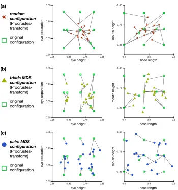
4.3 Examples of Procrustes-transformed MDS configurations . . . 47

4.4 Models fitted with MDSvs. original configurations . . . 48

5.1 Schematic diagram of HMAX early vision model . . . 52

5.2 HMAX S1 and C1 unit responses to a Brunswik face . . . 53

5.3 HMAX S2 unit responses to a Brunswik face . . . 54

viii LIST OF FIGURES

5.4 HMAX C2 unit responses for 12 sets of Brunswik faces . . . 55

5.5 Modifications to original HMAX model . . . 56

5.6 Correlations between HMAX C2 unit responses and stimulus features 57 5.7 HMAX C2 units that approximate original stimulus features . . . 58

5.8 Fidelity of HMAX representation as a function of number of C2 units 59 5.9 PCA reduction on HMAX C2 responses . . . 60

5.10 Four-dimensional PCA configuration from HMAX C2 responses . . . 61

6.1 Stimuli for eye-tracking experiments . . . 69

6.2 Free-viewing task used during eye tracking . . . 70

6.3 Eye-tracking setup . . . 72

6.4 Eye-tracking calibration accuracy . . . 73

6.5 Parsing a scanpath into fixations . . . 74

6.6 Salience model . . . 75

6.7 Method for comparing scanpaths with salience maps . . . 77

7.1 Short-range orientation interactions model . . . 83

7.2 Internals of the short-range orientation interactions . . . 84

8.1 Gabor arrays with and without embedded “snake” contours . . . 88

8.2 Contour-integration model . . . 90

8.3 Connection matrices in contour-integration model . . . 91

8.4 Contour-integration model with overhead imagery . . . 92

8.5 Contour-integration modelvs. edge-detection algorithms . . . 93

8.6 Contour-detection task used during eye tracking . . . 94

9.1 Mouse-clicksvs. eye fixations for overhead imagery . . . 104

9.2 Mouse-clicksvs. eye fixations for outdoor photos . . . 105

LIST OF TABLES

3.1 Model fits for categorization experiment 1 . . . 31

3.2 Model fits for categorization experiment 2 . . . 32

3.3 Qualitative comparison of categorization models . . . 34

5.1 Model fits for categorization experiment 2 . . . 62

6.1 Salience model fits for the free-viewing task . . . 78

6.2 Salience model fits as fractions of the theoretical maximum . . . 79

7.1 Salience model fits including short-range orientation interactions . . 85

8.1 Salience model fits for free-viewing task . . . 96

8.2 Salience model fits for contour-detection task . . . 97

9.1 Comparison of model fits for eye-tracking and mouse-click data . . . 101

Preface

The passing of a major milestone in life1_{is always an occasion for reflection,}

espe-cially when, as one colleague put it, “you have had about this much [holds hand about an inch in front of eyes] perspective on your research for the past six years.” Indeed the view is a bit different when one takes a step back: here is what I wrote (in part) as I applied for admission to the Computation and Neural Systems pro-gram at Caltech in fall of 1997:

I have always been fascinated by the great mysteries of nature, yet at times I have felt reluctant to single one out for further study, at the expense of being forced to neglect the others. Having realized, how-ever, that one cannot specialize in all the mysteries (except perhaps in kindergarten), and uneasy about the prospect of specializing in noth-ing at all, I decided upon a compromise. I embarked on a search for my center of intellectual gravity—that specialty that would be reinforced rather than undermined by my interests that formally lie outside the specialty.

I have performed this search by the admittedly haphazard proce-dure of reading one book, mulling it over, then moving on to what I fell impelled to read next. In the past year, this technique has taken me from (roughly in order)Ishmael(Daniel Quinn, 1992) toDreams of a Final Theory (Steven Weinberg, 1992), Shadows of the Mind (Roger Pen-rose, 1992),A Brief History of Time(Stephen Hawking, 1988),

Conscious-1_{If completing my Ph.D. doesn’t qualify as a major milestone, I have the impending rollover of}

a significant digit (who shall remain nameless) in my age to use as a backup milestone.

xii PREFACE

ness Explained (Daniel Dennett, 1991), The Language Instinct (Stephen Pinker, 1994),Darwin’s Dangerous Idea(Daniel Dennett, 1995), At Home in the Universe(Stuart Kauffman, 1995),The Extended Phenotype(Richard Dawkins, 1982),The Astonishing Hypothesis(Francis Crick, 1994),Elbow Room: The Varieties of Free Will Worth Wanting (Daniel Dennett, 1984),

The Intentional Stance(Daniel Dennett, 1987), Higher Superstitions(Paul Gross and Norman Levitt, 1994),The Tao of Physics(Fritjof Capra, 1975),

The Third Culture(John Brockman, 1995),The Embodied Mind(Francisco Varela, Evan Thompson, and Eleanor Rosch, 1991), The Quark and the Jaguar(Murray Gell-Mann, 1994), The Story of B (Daniel Quinn, 1996),

The Bell Curve(Richard Herrnstein and Charles Murray, 1994),The Mis-measure of Man(Stephen Jay Gould, 1996), andNeurophilosophy(Patricia Churchland, 1986). These sources, along with journal articles, some textbook reading, participation in online discussion groups, and con-versations with the world-class professors and peers that surround me at the University of Wisconsin, have led me to that center of intellectual gravity that has always been within me but only now apparent to me.

Daniel Dennett, in Consciousness Explained (1995), defines a mys-tery as “a phenomenon that people don’t know how to think about— yet.” From the human perspective, nature’s deepest mysteries have been those of origins: the origin of the universe and its physical laws, the origin of life, the origin of minds. Unifying these mysteries is the tantalizing question of how something could possibly come from noth-ing: how matter arises from the void, how complexity emerges from chaos, how subjective experiences derive from automata. These ques-tions have so baffled us that for most of our history only one solution has been remotely conceivable, in which each origin is seen as the man-ifestation of a new ontological category. Only recently have earnest attempts been made to explain these origins within the confines of the material world without separate ontological categories for life or for minds. Although smaller mysteries still surround aspects of each ori-gin, we are no longer entirely bewildered. The one remaining exception seems to be human consciousness, which as Dennett says, “is just about the last surviving mystery.”

special-PREFACE xiii

ization at all, for this is a broad subject legitimately claimed by a num-ber of traditional academic departments. Yet for reasons ranging from the entirely reasonable logistical demands of scientific research to occa-sional unintended ignorance, the theories within one department typi-cally span only a portion of the entire spectrum of thought surrounding the subject. And since no one department has yet been able to claim the one right way to think about the subject, I feel that the interdisciplinary nature of the developing cognitive science is of utmost importance. Al-though it imposes some obstacles in forcing one to become fluent in the jargon and pretheoretical conceptions of each of the component dis-ciplines, this can only strengthen the theories forged by the interdis-ciplinary coalition. Clearly I will be selecting a narrower focus than simply mind/brain studies for my graduate work, but I hope to main-tain a high level of competence in the interdisciplinary background that surrounds my focus.

I hope to participate in a future of cognitive science that I expect will be quite exciting and full of surprises. Patricia Churchland and Ilya Far-ber, in “Consciousness and the Neurosciences: Philosophical and The-oretical Issues” (inThe Cognitive Neurosciences, Michael Gazzaniga, ed., 1995), suggest that many of our current concepts about the mind are essentially prescientific, and awaiting us is a transition in which these concepts will be transformed and perhaps displaced by more precise and predictively powerful scientific concepts. Indeed, cognitive sci-ence is at a point where the right questions have yet to be asked, and a conceptual framework will evolve alongside the empirical answers that hang upon it. That science often proceeds this way is an important lesson.

xiv PREFACE

Russell, 1967): “I [believe] in the value of two things: kindness and clear thinking. . . . I find that much unclear thought exists as an excuse for cruelty, and that much cruelty is prompted by superstitious beliefs.”

It is to promote and practice kindness and clear thinking that I in-tend to pursue an academic career. In this capacity, the greatest respon-sibility is to internalize the process and the conscience of science, and to evidence these qualities in research and teaching. I firmly believe that when performed this way, science does good, whether its benefit to so-ciety be direct, such as through cures for disease, or indirect, through the expansion of humankind’s wisdom. I could not wish for more than to contribute to this cause through the study of the human mind, where a greater understanding would benefit us all on both personal and so-cietal levels.

ev-PREFACE xv

CHAPTER 1

Introduction

1.1 We open our eyes and see

We open our eyes and wesee.

It’s so simple. Yet the human visual system achieves such computational feats that to reproduce them with the conscious “I” would confound even the most prodigious mathematical mastermind. Our brain tells us “same” for the visage of a loved one, whether that face is seen in sunlight or firelight or starlight, whether seen from left, right, near or far, whether the face has aged by a few days or a few decades; yet, show us that same face next to its brother or sister, and our brain in-stantly tells us “different” even when the two faces are seen in precisely the same pose and lighting. Meanwhile, our eyes make on the order of 100,000 saccadic eye movements every day, masking the oft-forgotten fact of visual life that our visual acuity decays dramatically outside the central few degrees of the visual field.

Since it is the collective conscious “I” of all of us as scientists and engineers that designs artificial machine vision systems, such systems inherit a paradox that has plagued artificial intelligence: the tasks that are simple and efficient for human observers (such as identifying that loved one’s face) are monumental challenges for machine vision systems, while other tasks that are nearly impossible for hu-man vision (differentiating a “T” from an “L” in the periphery) are trivial for a computer program. Thus, machine vision and human vision currently have com-plementary strengths and weaknesses. But ultimately it is critical that machine vision systems be able to assist human observers even in tasks that are

2 CHAPTER 1. INTRODUCTION

ally human-friendly yet seem computationally intractable by today’s means. Recent developments in the computational neuroscience of vision have sug-gested an innovative technology for addressing these goals, that of neuroscience-enabled machine vision. This thesis describes work that aims to build a more con-crete understanding of the workings of specific mechanisms of the visual system, through a proof-by-example approach: we construct working computational mod-els and test whether they match the behavior of psychophysics subjects. If (when) the models pass this test, we have gained knowledge in the neurobiology of vision, and along the way we may have built a better machine vision system as well.

Nature is fond of arranging things in twos, and the visual system is no excep-tion: starting from two eyes, the world is split into two (left and right) visual half-fields, information from each being sent to two separate half-brains. Millions of years of evolution in the presence of a ubiquitous visual horizon has taught the brain to further split the world into upper and lower visual half-fields (and to pay extra attention to the lower one). From the retina, visual information also begins a divergence into two parallel processing streams, one (roughly) for motion and spatial judgments, and one for shape and color; these are variously named as the

where/what, ormagno/parvo, oraction/perception, or dorsal/ventralpathways [ Schnei-der, 1969,Ungerleider and Mishkin, 1982, Mishkin et al., 1983,Goodale and Mil-ner, 1992, Milner and Goodale, 1993, Tanaka and Shimojo, 1996]. These parallel streams provide the top-level structural organization of this thesis, which contains two main parts: the first addresses visual object categorization, or how do we know what we’re looking at?, and the second addresses visual attention how do we know where to look?

1.2 Categorization

dif-1.2. CATEGORIZATION 3

ferent shapes or different constituent features. The basic-level category is avisual

category, not a linguistic or semantic one, because categories occupying the same linguistic level are not always at the same visual level. In an oft-cited example, when people are asked to name a picture of a bird, they will likely respond with “bird,” unless the picture contains an ostrich or a penguin, in which case they will be veryunlikelyto respond with “bird,” but rather will use the more specific term (unless they are bird experts; seeTanaka and Taylor, 1992). This can be explained by the fact that most birds do share a common shape, while those species that are exceptions to the rule will belong to a separate basic-level category. Other exam-ples of basic-level visual categories are human faces, four-door sedan automobiles, jogging shoes, and ball-point pens.

At levels higher than the basic level, the hierarchy of categories ultimately ex-tends out of an exclusively visual domain and into the linguistic domain, where we find categories like animals, plants, chairs, and food. Here we find objects likesteak sandwichandfruit saladthat, despite sharing few visual characteristics, are both as-sociated with the same category label “food.” Objects of these superordinate-level categories can be identified and named on the basis of visual evidence, to be sure, but the category boundaries are not learned by strictly visual means.

Moving in the other direction through the hierarchy, more detailed than the basic-level category is the level category. Examples of subordinate-level categories include male faces and female faces (subordinate categories of the basic-level category of human faces) as well as different models of four-door sedan. In addition to sharing a similar shape and set of features, members of a subordinate-level category also typically share a common spatial arrangement of those features. On the other hand, members of different subordinate-level cate-gories within the same basic-level category are distinguished from each other by having different spatial arrangements of the same features. This is the level that is associated with expertise; in fact a common definition for visual expertise in a certain domain is the ability to perform subordinate-level tasks with the same speed and precision as basic-level tasks. Thus it is said that we are all natural-born experts at face recognition, for upon viewing a face we recall the person’s name just as quickly as we identify the fact that it is a face in the first place. The same characteristic is found in trained experts in other fields, such as car enthusiasts or bird watchers. Some evidence from fMRI suggests that the samefusiform face area

4 CHAPTER 1. INTRODUCTION

1999,2000b,a,Tarr and Gauthier,2000].

Part I of this thesis focuses on computational models of subordinate-level cate-gorization. We begin in Chapter2by introducing several simple sets of schematic, line-drawn objects, each sharing a common set of features and differing in the spatial arrangements of those features. Subsequent chapters explore the ways in which such stimuli might be processed by the visual system: how the raw sensory input from the retina is transformed into a compact intermediate representation (Chapter5), what the nature is of this intermediate representation (Chapter4), and finally how this representation can be used to reach a categorization decision about the input stimulus (Chapter3).

1.3 Attention

A neuron anywhere in the visual system undoubtedly exemplifies another of na-ture’s dichotomies: bottom-up and top-down influences. Bottom-up processes are typically thought of as stimulus-driven, unconscious, automatic, not subject to voluntary control, and produced by anatomical feed-forward connections. Ex-amples of bottom-up processes in vision include the detection of a flash of light, the “pop-out” of a red object amongst a green background, or the identification of a face. Jerry Fodor [1985] has used the termcognitively impenetrableto describe early bottom-up processes: we cannot voluntarily alter them, and furthermore we can-not determine the mechanisms for their action by introspection. Although bottom-up visual processing seems subjectively simple because it requires no voluntary effort and is cognitively impenetrable in any case, any computational neurosci-entist or machine vision engineer will attest that the underlying mechanisms are far from simple. In a metaphor from computer programming, this is classic infor-mation hiding: the visual system shields the conscious “I” from a mass of imple-mentation complexity with a trivially simple interface (i.e., we open our eyes and

see).

1.3. ATTENTION 5

without delay. Another common example of top-down processing is the Rorschach inkblot test, in which people are shown inkblots that have no “true” interpreta-tion, yet high-level cognitive states force an interpretation of the image from the top down.

Part I

Visual object categorization

CHAPTER 2

Categorization psychophysics with

parametric stimuli

2.1 Introduction

Visual object recognition and categorization are critically important to the survival of many animal species, notably humans. These processes constitute an impres-sive computational feat, in that we are able to, on the one hand, lump together as “same” a set of views of an object seen under different conditions that produce radically different patterns of light on the retina, yet on the other hand, mark as “different” two views of different objects under similar viewing conditions that produce very similar patterns of light falling on the retina.

In the last thirty years, research in mathematical psychology has discovered much about the processes of visual categorization [e.g.,Reed,1972,Nosofsky,1984, 1991,Ashby,1992a,Ashby and Maddox,1993,Smith and Minda,1998,Ashby and Waldron, 1999] by combining the techniques of visual psychophysics and compu-tational modeling to develop high-level theories of categorization. Despite the predictive success of these theories, there exists a gap between the descriptive framework of the models, and our current knowledge of the neuronal mechanisms involved in categorization. An important aim therefore is to shorten this gap by ex-tending models so that their implementations are reasonable in light of recent de-velopments in the neurophysiology of object recognition and categorization [ Kan-wisher, McDermott, and Chun, 1997, Ishai, Ungerleider, Martin, Schouten, and

10 CATEGORIZATION PSYCHOPHYSICS

Haxby, 1999, Freedman, Riesenhuber, Poggio, and Miller, 2001,Sigala and Logo-thetis, 2002,Op de Beeck, Wagemans, and Vogels,2001,Ashby and Ell,2001].

Most categorization models assume, perhaps tacitly, a categorization process in which

• the immediate sensory representations of incoming stimuli occupy a very high-dimensional space (for vision, this comes to millions of dimensions when we consider that output of each retinal ganglion cell amounts to a sin-gle dimension);

• this very high-dimensional representation is transformed into an intermedi-ate space of lower dimensionality by combining the simple features of the early representation (such as oriented edges) into more complex features (such asT- orL-junctions or simple shapes);

• finally, a computational process operates in this lower-dimensional space and produces an explicit categorization result that can be the basis for a behav-ioral response (such as a button-press in a psychophysics experiment).

Here, we address each of these three key steps with categorization models in-formed by psychophysics experiments and neurobiology. We will visit the topics in reverse order: our goal is to describe how a categorization decision is made for a visual object, and each of the next three chapters takes a step toward filling in the details of this process back to the retinal input. First, in Chapter3we compare sev-eral existing models of visual object categorization and introduce a newroaming ex-emplar model(RXM) that highlights the importance of certain model characteristics in matching human behavior. Second, in Chapter4we delve into the nature of the intermediate representation using multidimensional scaling(MDS). Third and last, many models in the psychological literature ignore the transformation which turns raw sensory data into a succinct set of nameable features; we explore this step in detail in Chapter5using a model of early vision similar to “HMAX” [Riesenhuber and Poggio,1999] to drive subsequent phases of the categorization process.

2.2. PSYCHOPHYSICAL METHODS 11

2.2 Psychophysical methods

Like many other studies of visual object categorization, we used schematic line-drawn stimuli. Many insights into the principles of categorization have been ob-tained with minimalistic stimuli, such as the circles shown in Figure 2.1. We used three types of schematic, line-drawn visual stimuli with somewhat more complex-ity (Figure 2.2): Brunswik faces and tropical fish outlines, which have been used previously, plus a new set of “cartoon face” images. Each type of visual object was parameterized along four dimensions comprising thestimulus parameter space. For each object type, different sets of objects were assigned toconfigurations, which contained equal numbers oftraining exemplarsassigned to each of two categories, as well as an additional number oftest exemplars. The training exemplars from the two categories were always chosen so as to be linearly separable in the objects’ parameter space; that is, the members of the two categories could be separated by some 3-D hyperplane in the 4-D parameter space.

d θ

Figure 2.1. An example of the type of parametric stimuli used in previous studies [e.g.,

Maddox and Ashby,1993] of visual object categorization. In this example, the objects are

circles with a bisecting line defined by two features: the diameterd of the circle and the

angle θ of the bisecting line. Experiments using these stimuli typically involve categories

devised so that both features must be analyzed in order to determine category member-ship. For example, category 1 might include all small circles as well as some medium-sized circles with nearly-horizontal bisectors, while category 2 would include all large circles as well as medium-sized circles with nearly-vertical bisectors. In such an experiment, the question of interest would be to quantitatively understand how observers categorize the ambiguous objects of medium size with diagonal bisectors.

2.2.1 Brunswik faces

mon-12 CATEGORIZATION PSYCHOPHYSICS

keys,Sigala et al.,2002). Each face consists of a simple ovaloid outline with internal features defined by (compressed) circles and straight lines. The faces are parame-terized byeye height (EH; the vertical distance from the centers of the eyes to the center of the face),eye separation(ES; the horizontal distance separating the centers of the eyes),nose length(NL; the vertical length of the nose line), andmouth height

(MH; the vertical distance from the center of the face to the mouth line).

2.2.2 Cartoon faces

These stimuli (Figure 2.2b) were introduced in an fMRI study [Jovicich, Peters, Koch, Chang, and Ernst,2000] that showed them to produce stronger activation in the human fusiform face area [Kanwisher et al.,1997] than did Brunswik faces (see Section2.3below). The cartoon faces extend the Brunswik faces in several ways to make the faces appear more human: a simple band of hair is added around the top of the head, the size and dilation of the pupils may be varied, eyebrows are added above the eyes, the nose outline is defined by an extended open contour, and the mouth is defined as a Bezier curve rather than a straight line. To control these addi-tional features, the cartoon faces have a total of 28 stimulus parameters; however, in the present study only the four parameters corresponding to the Brunswik face dimensions were varied, while the other 24 parameters were held constant.

2.2.3 Tropical fish outlines

These line-drawn images (Figure2.2c) were first used to offer a completely novel stimulus set to monkey observers in a categorization task [Sigala et al.,2002]. Other fish images have been used previously in studies of categorization in people and pigeons [Hernstein and de Villiers,1980] and in monkeys [Vogels,1999]. Each fish image is composed of four cubic spline curves that were fitted to scanned outlines of tropical fish. By adjusting one control point of each of the curves, four features of the outlines could be smoothly deformed: the dorsal fin (DF), tail fin (TF), ventral fin (VF), and mouth area (MA).

2.2.4 Stimulus rendering

All of the stimuli described here were generated and displayed to subjects

us-ing GroovX, a custom software software designed for psychophysics and

Li-2.3. NEURAL REPRESENTATION OF SCHEMATIC STIMULI 13

(a) Brunswik faces

(b) Cartoon faces

(c) Fish outlines

(EH) Eye height

(ES) Eye separation

(NL) Nose length

(MH) Mouth height

(EH) Eye height

(ES) Eye separation

(NL) Nose length

(MH) Mouth height

(DF) Dorsal fin

(TF) Tail fin

(VF) Ventral fin

(MA) Mouth area ES

ES

TF DF

VF MA

EH

EH

NL NL

MH

MH

Figure 2.2. Three object types, each with four stimulus parameters controlling that object

type, were used in similarity and categorization psychophysics tasks. Three sample ob-jects of each type demonstrate the typical ranges of the parameters. (a) Brunswik faces.

(b) Cartoon faces. Although these faces are described by 28 parameters, the present

study used only the 4 parameters corresponding to those in (a). (c) Fish outlines.

cense (GPL), and is freely available for download from the internet. Currently documentation and source code may be found online at this web address: http:

//www.klab.caltech.edu/rjpeters/groovx/. In the event that this software later

moved to a different location it should be locatable via a number of popular inter-net search engines using the keywordGroovX.

2.3 Neural representation of schematic stimuli

14 CATEGORIZATION PSYCHOPHYSICS

>

L

R

L

R

L

R

L R

L R

L R

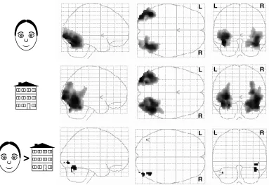
Figure 2.3. BOLD activity observed with fMRI while subjects viewed photos of either faces

(top row) or houses (middle row), and the contrast between two conditions showing regions which were more active during face viewing (bottom row). This contrast reveals bilateral activation in the lateral occipital cortex (LO) and fusiform face area (FFA).

2.3. NEURAL REPRESENTATION OF SCHEMATIC STIMULI 15

>

L

R

L

R

L

R

L R

L R

L R

Figure 2.4. Same conditions as in Figure2.3, except that cartoon faces and cartoon house were used in place of the photos. Compared to the condition with face and house photos, activation here in LO and FFA is reduced on the right side, and is nearly absent on the left side.

viewing). Activation was defined as the difference in the signal changes between the face and house conditions. For each subject, data were scaled to the global brain mean and analyzed separately to locate the areas which responded more to faces than to houses during the different stimuli sequences. The strength of the effect was then averaged in these areas across subjects for each condition.

When we looked for areas that were significantly more activated by photos of real faces than by photos of real houses (Figure 2.3)1, we found strong bilateral activation in the lateral occipital (LO) cortex (p < 0.001, uncorrected) as well as in the inferior temporal gyrus consistent with the FFA (p < 0.001, uncorrected). For comparison with the Brunswik and cartoon faces, we designed schematic house stimuli with different levels of complexity to match the subjective complexity of the different face stimuli. In the analogous face/house comparisons, we found FFA activation for the cartoon faces that was strongly right-side dominant (Figure2.4), and we found no detectable FFA activation for the Brunswik faces (Figure 2.5). This does not rule out the possibility that Brunswik faces activate neurons in the

16 CATEGORIZATION PSYCHOPHYSICS

>

L

R

L

R

L

R

L R

L R

L R

Figure 2.5. Same conditions as in Figures 2.3and 2.4, except that Brunswik faces and simple house cartoons were used. No activation was observed in either LO or FFA.

CHAPTER 3

Categorization models

3.1 Introduction

This chapter describes a number of models that attempt to mimic human catego-rization decisions using a mechanism based on the multidimensional representa-tion of incoming stimuli, plus possible auxiliary representarepresenta-tions, such as mem-ory traces. This process is typically controlled by a number of free parameters, which are fitted with the goal of matching human categorization behavior. How-ever, a simple statistical comparison between models—even after accounting for the number of free parameters—may ignore important differences in the neurobi-ological implications of the models. For example, one successful model, the gener-alized context model (GCM; Nosofsky, 1984), assumes that all training images are stored in memory; a literal interpretation of the GCM might conclude that the neuronal substrate of categorization also scales linearly with the number of ex-emplars in a category, or that categorization in biological systems involves only simple memorization, without any category-level abstraction [Knowlton, 1999]. To provide a more detailed look at such issues, we introduce a roaming exemplar model(RXM) that draws from neural networks [Poggio and Girosi, 1990, Rosseel, 1996] and exemplar-based models of categorization [Nosofsky, 1991, Kruschke, 1992,Nosofsky, Kruschke, and McKinley,1992]. The RXM also has much in com-mon with thestriatal pattern classifier(SPC) ofAshby and Waldron [1999], includ-ing the fact that its memory traces are free parameters. This stands in contrast to previous exemplar-based models, and hence neurobiological plausibility can be

18 CHAPTER 3. CATEGORIZATION MODELS

assessed directly by accounting for numbers of free parameters when comparing fitted models.

3.2 Categorization psychophysics tasks

Subjects participated in categorization experiments consisting of a training phase and a testing phase. In both phases, subjects viewed a series of objects presented one at a time. Each object was shown for 2 s, followed by 2 s of blank screen. Dur-ing each 4 s trial, subjects pressed one of two buttons indicatDur-ing to which category the object belonged. In the training phase, subjects were shown only the two cate-gories’ training exemplars, and were given feedback in the form of a high- or low-pitch tone indicating whether their response was correct or incorrect, respectively. Subjects performed training blocks of 100 trials until they scored ≥ 85% correct on a single block. Next, they moved into the testing phase, in which they were shown the previously unseen test exemplars in addition to the training exemplars that they had viewed during the training phase. Subjects received no feedback on their responses during the testing phase.

In Experiment 1, the values for each stimulus dimension were quantized to three possible values for each dimension, so that the set of possible objects lay on a 3×3×3×3 grid in stimulus parameter space. The configuration of 20 objects on this grid (Figure 3.1a) followed that used in Nosofsky [1991] and Sigala et al. [2002], with five training exemplars for each category, plus ten test exemplars that included the two category prototypes. For each set of objects, each of the four stimulus parameters for that object type was assigned to one of the four generic dimensions in the stimulus configuration shown in Figure 3.1a. It is significant how the parameters are assigned, since each generic dimension carries different information about category membership. For example, the categories were lin-early separable in projections onto 2-D planes for pairs of stimulus dimensions

(1, 2), (1, 3), and (1, 4), so dimension 1 was more informative about an object’s

category than were the other dimensions. In all, five sets of stimuli were used in Experiment 1. These included three sets of Brunswik faces in which the stimulus parameters were assigned to the generic dimensions in different orderings ({EH, ES, NL, MH}, {NL, MH, EH, ES}, and{MH, EH, NL, ES}), a set of cartoon faces ({EH, ES, NL, ML}), and a set of fish outlines ({TF, VF, DF, MA}). The twenty ob-jects in each of these configurations are shown in Figures3.2,3.3,3.4,3.5, and3.6.

3.2. CATEGORIZATION PSYCHOPHYSICS TASKS 19

10 training exemplars for each of the two categories, plus 60 test exemplars. The exemplars were arranged on a 7×7×7×7 grid in the stimulus parameter space. There were 12 such sets, identical except that the discretization grid of each set was rotated through different angles (θ = n·15◦,n ∈ [0 . . . 11]) in the

eye-height/eye-separation plane of parameter space.

d im e n s io n 2 d im e n s io n 3 d im e n s io n 4

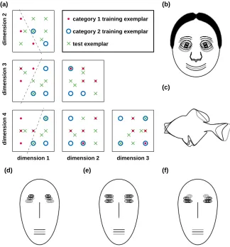
dimension 1 dimension 2

category 1 training exemplar

category 2 training exemplar

test exemplar dimension 3 (a) (b) (c) (f) (e) (d)

Figure 3.1. Experiment 1 used five 20-object sets, each defined in a 4-D parameter space. (a) The abstract configuration is shown in projections onto the six possible pairs of

dimen-sions. All exemplars fall on a 3×3×3×3 grid, except for the two category prototypes, which

were among the test exemplars. Dashed lines indicate where the two categories’ training exemplars are linearly separable. (b-f) For illustration, the training exemplars of category one (thin black lines) are superimposed upon those of category two (thick gray lines).

(b) Cartoon faces with dimensions {1=EH, 2=ES, 3=NL, 4=ML} (see also Figure 3.2).

(c) Fish outlines {TF, VF, DF, MA} (Figure 3.3). (d) Brunswik faces {EH, ES, NL, MH}

(Figure 3.4). (e) Brunswik faces {NL, MH, EH, ES}(Figure 3.5), and (f) Brunswik faces

20 CHAPTER 3. CATEGORIZATION MODELS

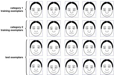
category 1 training exemplars

category 2 training exemplars

test exemplars

Figure 3.2. Cartoon faces{EH, ES, NL, ML}used in experiment 1.

category 1 training exemplars

category 2 training exemplars

test exemplars

3.2. CATEGORIZATION PSYCHOPHYSICS TASKS 21

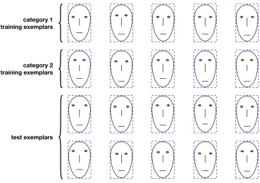
category 1 training exemplars

category 2 training exemplars

test exemplars

Figure 3.4. Brunswik faces{EH, ES, NL, MH}used in experiment 1.

category 1 training exemplars

category 2 training exemplars

test exemplars

22 CHAPTER 3. CATEGORIZATION MODELS

category 1 training exemplars

category 2 training exemplars

test exemplars

3.3. CATEGORIZATION MODELS 23

0º 15º 30º 45º

60º 75º 90º 105º

120º 135º 150º 165º

Figure 3.7. Experiment 2 used these 12 sets of Brunswik faces. Each image shows the

10 training exemplars of category one (thin black lines) superimposed upon the 10 training exemplars of category two (thick gray lines). The sets differ only in the angle by which the objects are rotated in eye height-eye separation plane of feature space.

3.3 Categorization models

24 CHAPTER 3. CATEGORIZATION MODELS

the neurobiological plausibility of the different models.

In general, the categorization models assume the following:

• that each exemplarxhas a unique representation in an R-dimensional space [Ashby,1992b],

x= (x1, . . . ,x_R),

whose components may be drawn either from the original stimulus config-uration, from a multidimensional scaling configuration (see Chapter 4), or from a configuration based on features extracted from an early-vision model (chapter5), and

• that each category is defined by Ntraining exemplars

{x1, . . . ,x_N}.

3.3.1 Exemplar models

Exemplar models associate memory traces of M (with 1 ≤ M ≤ N) stored exem-plars1

{y₁, . . . ,y_M}

with each category. Several model subtypes differ in the way that these stored exemplars are selected:

• All-exemplar models (Figure 3.8a) assume M = N, and y_i = x_i. All of the

training exemplars are explicitly stored in memory, so these models have a high memory demand that is linear in the number of training exemplars. All-exemplar models include the average-distance model (ADM, Reed, 1972) andgeneralized context model(GCM;Nosofsky, 1991).

• Prototype (one-exemplar) models (Figure 3.8b) assume M = 1; each category

stores only the arithmetic mean of the category’s training exemplars, y₁ =

1

N ∑ixi. These models have low and constant memory demand, independent

of the number of training exemplars; however, the models imply a more com-plex computational mechanism to estimate the prototype during trial-by-trial

1_{Our usage of the term “exemplar” to denote stored memory traces reflects a meaning ofideal}

meaning or patternorprototype, rather than a strict meaning ofprevious seen stimulus. For example,

3.3. CATEGORIZATION MODELS 25

stored exemplar/prototype training exemplar

category 1:

training exemplar stored exemplar/prototype

category 2:

test exemplar

cv₁=

3/4

cv₂=

1/4

cv₁=1/3

cv₂=2/3

d

P₁ S1-2

S_2-2

S_1-1

S_2-1

P₂

(a) all-exemplar model (b) one-exemplar model (prototype model)

(c) roaming exemplar model〈2〉; striatal pattern classifier〈2〉

(e) cue-validity model (d) linear boundary model

Figure 3.8. Schematic depictions of several kinds of categorization models. Each

dia-gram shows a hypothetical set of training exemplars from two categories (• and ◦) in a

2-D feature space, plus a test exemplar (×) which is to be classified. (a,b,c) Three types

of models which rely on distances (indicated by dashed lines) between a test exemplar and each stored exemplar from both categories: (a) all-exemplar model, in which the set of stored exemplars is just the set of training exemplars; (b) one-exemplar, or prototype

model, in which the single stored exemplar per category is the arithmetic mean of that

cat-egory’s training exemplars; (c) roaming-exemplar modelhMi(RXMhMi) and striatal pattern

classifierhMi(SPChMi), in which each category hasM(in this case,M =2) stored exem-plars, which must lie within the polygon that circumscribes the training exemplars (dotted

lines). The RXMhMi uses a summed-similarity decision rule, while the SPChMi uses a

uses a nearest-neighbor decision rule. (d) Linear boundary model, in which the model uses a linear boundary that separates the categories to classify test exemplars according to the side of this boundary on which they fall. (e) Cue-validity model, which classifies a

test exemplar according to the total cue-validity across all features; the cue-validitycv_i for

category i of a given feature is the posterior probability of an exemplar with that feature

26 CHAPTER 3. CATEGORIZATION MODELS

exposure to the training exemplars. Prototype models include the weighted prototype model(WPM;Reed,1972) and theweighted prototype similarity model

(WPSM;Nosofsky, 1991).

• In the proposedroaming-exemplar modelhMi(RXMhMi, Figure3.8c), each cat-egory storesMexemplars, each of which is a linear combination of the train-ing exemplars for that category, y_j = ∑_iw_ijx_i. Under the neurobiological consideration that neurons do not represent objects far different from those that have been previously observed, the stored exemplars are restricted to a region circumscribed by the training exemplars, so the weights are con-strained byw_ij ≥0 and ∑_iw_ij = 1 for allj. The number of stored exemplars

M isnota free parameter of a given RXMhMi, but the stimulus parameters of those stored exemplarsarefree parameters of the model. Thus, when the RXM is fitted to a dataset, the number of stored exemplars is chosen and fixed at the start, although RXMhMi’s with different (fixed) values ofMmay be fitted to the same dataset. The memory demand of the RXMhMivaries be-tween that of the prototype models (for M = 1) and that of the all-exemplar

models (for M = N); the computational complexity is similar to that of the

prototype models, since some mechanism must adjust the stored exemplars during training.

Next, the exemplar model computes a similarity measure between the test ex-emplar xand each of the stored exemplarsy, based on a weighted Euclidean dis-tance:

dα(x,y) = s

∑

j

α_j(x_j−y_j)2,

with α_j ≥ 0 and ∑α_j = 1 (other metrics are possible; e.g., Ashby and Maddox

1993). The coefficientsα_j, calledattentional weights, are intended to model the

abil-ity of human observers to attend preferentially to the most task-relevant stimulus features. The similaritys decays with the distanced, either linearly (s = −d, as in the RXM, ADM and WPM), or exponentially (s =e−cd, as in the GCM and WPSM;

seeShepard,1987).

Then, for each test exemplar x, the evidence E_i for category C_i is given as the sum of similarities betweenxand theMstored exemplarsyi

jof that category:

E_i(x) =

∑

j=1

3.3. CATEGORIZATION MODELS 27

Finally, the model’s categorization ofxis based on the expression

E1(x)−E2(x) +n> t,

where nrepresents zero-mean Gaussian noise with varianceσ2, and tis a

thresh-old parameter; x is assigned to category 1 if this expression is true, otherwise to category 2.

The free parameters of the exemplar models are thus(α,c,t,σ), plus 2Mstored

exemplars for the RXMhMi.

3.3.2 Striatal pattern classifier

The RXM shares a very similar mathematical formulation with the striatal pattern classifier(SPC) proposed byAshby and Waldron[1999], although the mathematical elements have been treated with different neurobiological interpretations [Ashby and Ell, 2001]. Both kinds of model rely on a set of units that represent different locations in feature space, but the models differ in how each category’s evidence is computed for a given test exemplar. The exemplar models compute the sum of similarities between the test exemplar and each stored exemplar, whereas the SPC associates a test exemplar with the category of the nearest striatal pattern (in this respect the SPC resembles a k-nearest neighbor model withk = 1). Both the

SPC and the RXM use a similarity measure that decays linearly with distance. In order to maintain a formal similarity with the other models, we used the following decision rule for the SPC: for each test exemplar, the evidence for each category is given by the maximum of the similarities between the test exemplar and that category’s stored exemplars. Thus, in the case of one stored exemplar per category, the SPCh1iand the RXMh1iform identical decision surfaces. However, withM > 1, the SPChMihas a piecewise-linear boundary, while the RXMhMi has a curved decision boundary.

3.3.3 Boundary models

proba-28 CHAPTER 3. CATEGORIZATION MODELS

bility densities) falls along the intersection of the graphs of the two probability density surfaces. If the covariance matrices of the exemplar distributions are iden-tical for the two categories, then the decision boundary is a linear surface (i.e., a hyperplane); otherwise, it is a quadratic surface.

We tested the probit linear model (PBI; Figure 3.8d; Ashby and Gott, 1988), which is trained to separate the categories’ training exemplars with a boundary described by a normal vectorband a thresholdt. Following training, a test exem-plarxis classified according to the side of the boundary on which it falls:

x·b+n >t ⇒x ∈C₁

The PBI model parameters are (b,t,σ); however the variance of the noise is

as-sumed to be σ2 = 1, since for any λ 6= 0, the two models given by (b,t,σ) and (λb,λt,λσ)are identical.

3.3.4 Cue-validity models

Cue-validity models (Figure3.8e) treat each stimulus parameter as an independent indicator of category membership, based on the relative numbers of exemplars from the two opposing categories that exhibit thecue(a particular value of a stim-ulus parameter). Thus, for example, a beard is a somewhat uncommon feature of male faces, yet it is an even less common feature of female faces, and so provides a highly valid cue to the gender category of a face.

In the weighted cue-validity model (WCVM;Reed,1972), the validity for cate-goryCiof the j-th parameter xjof a test exemplarxis defined as

v_ij(x) = p(C_i|x_j).

The overall cue-validityV_i is a weighted sum of these validities,

V_i(x) =

∑

j

α_jv_ij(x),

where the α_j are attentional weights as in the exemplar models, with α_j ≥ 0 and

∑_jαi = 1. Also as in the exemplar models, the decision rule incorporates Gaussian

noisenand a thresholdt; if the expression

3.4. MODEL FITTING 29

is true,xis assigned to category 1, otherwise to category 2.

A modified version of this model, called the weighted frequency cue-validity model (WFCVM;Reed,1972), uses a different definition for the validity. A weight factor,

q = 1

1+F(x_m),

is computed from the overall number of timesF(xm)that the parameter value xm

occurs in exemplars from both categories. Then the WCVM’s original validity v_ij

is used to define the new validity

˜

v_ij(x) = 1₂·q+v_ij(x)·(1−q),

so that the validities of rare parameter values carry little information about cate-gory membership. This reflects the idea that subjects will pay more attention to common features.

The free parameters for both the WCVM and the WFCVM are(α,t,σ).

3.4 Model fitting

We fitted models based on several alternative representations for the schematic stimuli:

• the objects’ physical parameter values (discussed in this chapter),

• the psychophysical parameter values obtained from multidimensional scal-ing (see Chapter4), and

• the features derived an early vision model (Chapter5).

Furthermore, each model could either be fitted separately to each individual sub-jects’ data, or be fitted once to data pooled across subjects. However, since pooled fits may not accurately reflect the categorization processes of individual observers [Maddox,1999], we used only models fitted to individual subjects’ data.

30 CHAPTER 3. CATEGORIZATION MODELS

set of observed probabilities p_i, given the values of the model parameters (which govern the predicted probabilities ˆp_i), over theNstimulus objects:

L =

N

∏

i=1

n

i

p_in_i

(pˆ_i)pini₍1₋pˆ_i)(1−pi)ni,

where n_i is the number of categorization trials performed for objecti, and p_in_i is the number of trials in which the observer assigned object i to category one. The likelihood takes the form of a binomial distribution because subjects’ responses are treated as independent binary random variables. A numerical implementa-tion of adaptive simulated annealing [Ingber,1989] followed by a simplex method [Nelder and Mead,1965] was used to maximize the likelihood L, or equivalently, minimize the minusloglikelihood(−lnL), which can be computed more efficiently. The range of the likelihood is 0≤ L≤1, so the range of the minus loglikelihood is

∞ _{≥ −}lnL_≥0.

We used the percentage of variance (%-variance) explained by the model as a more tangible measure for comparing fitted models. This measure is simply given byr2_{, the square of the correlation coefficient between the observed and predicted} probabilities.

Finally, although the loglikelihood (lnL) or %-variance are appropriate statis-tics for comparing fitted models having similar numbers of free parameters, com-parisons of models differing in their number of free parameters, Nfp, require a statistic such as the Akaike information criterion [Zucchini,2000],

AIC= −2 lnL+2N_fp,

which contains a penalty term proportional to N_fp. Pairwise model comparisons were made with the Wilcoxon signed-rank test of either−lnLor the AIC, and we report the median value of −lnL or the AIC to summarize the model fits from a group of individual subjects.

3.5 Model fits: Experiment 1

3.5. MODEL FITS: EXPERIMENT 1 31

Table 3.1. Goodness-of-fit of the categorization models tested in Experiment 1.

GCM PBI WPSM WCVM

Brunswik faces{EH, ES, NL, MH} % variance 98.22 98.08 96.39 88.37

−lnL 21.15 22.23 27.32∗ 42.50∗ Brunswik faces{NL, MH, EH, ES} % variance 95.68 97.75 95.32 74.38

−lnL 28.08 26.53 32.81 42.58∗ Brunswik faces{MH, EH, NL, ES} % variance 94.02 58.56 61.55 86.30

−lnL 36.83 80.57∗ 90.31∗ 52.76 cartoon faces % variance 95.50 90.70 90.18 86.66

−lnL 30.68 29.95 37.07∗ 53.49 fish outlines % variance 97.23 80.98 70.30 96.03

−lnL 20.73 32.85∗ 74.36∗ 28.74

% variance (larger value indicated better fit)

−lnL, minus loglikelihood (smaller value indicates better fit) bold numbers, model(s) which gave the best fit in each row

∗, models whose−lnLwas significantly worse (p<0.05_{) than the best-fitting model in each row}

or GCM).

Table 3.1 summarizes the fits of the all-exemplar, linear boundary, prototype, and cue-validity models, for each of the five sets of objects used in Experiment 1, along with significance values for pairwise comparisons of the models using the Wilcoxon matched pair signed rank test2_{. There were two general patterns of}

model fits.

The first pattern was associated with the first two Brunswik face sets ({EH, ES, NL, MH} and {NL, MH, EH, ES}, which depend primarily on attention to the eyes and nose) and the cartoon faces ({EH, ES, NL, ML}). In this pattern, the all-exemplar models obtained the best fit, but the boundary model also fit well, in-distinguishable from the exemplar models. The prototype models fit significantly worse (p < 0.05) than the all-exemplar models, but the magnitude of this differ-ence was small. Finally, the cue-validity models fit significantly worse than the other models.

The second pattern was seen with the third Brunswik face set ({MH, EH, NL, ES}) and the fish outlines ({TF, VF, DF, MA}). As in the first pattern, the all-exemplar models obtained the best fit. However, the rest of the pattern was quali-tatively different from the first pattern. Whereas the cue-validity models gave the worst fits in the first pattern, their fits were indistinguishable from the all-exemplar

2_{Note that the RXM and SPC were not used in fitting the data from Experiment 1 because even}

32 CHAPTER 3. CATEGORIZATION MODELS

Table 3.2. Goodness-of-fit of the models tested in Experiment 2. See also Table 3.3for further discussion of the models’ qualitative properties.

RXMh1i RXMh2i RXMh3i SPCh1i SPCh2i SPCh3i GCM PBI WPSM

% variance 89.36∗ _90.98∗ _{91.49 89.36}∗ _90.83∗ _{91.64 86.84}∗ _87.10∗ _84.90∗

−lnL 75.72∗ 72.06∗ 71.32∗ 75.72∗ 71.65∗ 69.92 83.41∗ 83.66∗ 88.79∗

AIC 173.44 178.13∗ 188.64∗ 173.44 177.30∗ 185.84∗ 178.81∗ 177.32 189.57∗ % variance (larger value indicated better fit)

−lnL, minus loglikelihood (smaller value indicates better fit) AIC, Akaike Information Criterion (smaller value indicates better fit)

bold numbers, model(s) which gave the best fit in each row

∗, models whose fits were significantly worse (p<0.05) than the best-fitting model in each row

models in the second pattern. In addition, the boundary model fit very poorly, significantly worse than the exemplar models (p < 0.05). Finally, the prototype models fit even more poorly, significantly worse than the exemplar and boundary models (p <0.05).

3.6 Model fits: Experiment 2

We fitted subjects’ categorization probabilities from Experiment 2 with versions of the roaming-exemplar model and striatal pattern classifier using 1, 2, 3, 5, 7, and 10 stored exemplars3, as well as the all-exemplar, prototype, and linear boundary models, and assessed these fits with three measures (see Table 3.2): the loglikeli-hood, the %-variance explained, and the Akaike information criterion (AIC).

When the model fits were assessed with their minus loglikelihoods (Table 3.2, row 2), we observed a pattern among the previously tested models similar to the first pattern observed in Experiment 1: the all-exemplar and boundary models both obtained better (lower) scores than the prototype model. However, each of these previous models was outperformed by all versions of the roaming-exemplar model and striatal pattern classifier. In addition, for both the RXMhni and the SPChnithe goodness of fit increased with the number n of stored exemplars—an unsurprising result, given that each stored exemplar reflects additional free pa-rameters. The %-variance values (Table3.2, row 1) show a similar pattern, but give a more concrete assessment of how well the models match the human subjects’ categorization behavior: the best-fitting model (the SPCh3i) captured nearly 92%

3_{For brevity, the models with 5, 7, and 10 stored exemplars were withheld from Table3.2, since}

3.7. DISCUSSION 33

of the variance, while the worst-fitting model (the WPSM) captured roughly 85% of the variance.

In contrast, when the model fits were assessed with the AIC to account for their numbers of free parameters (Table3.2, row 3), the RXM and SPC with one stored exemplar per category (RXMh1i and SPCh1i) obtained the best (lowest) scores among all models. These comparisons were statistically significant (p < 0.05, Wilcoxon signed rank test) except against the PBI (p =0.44). Moreover, increasing

the number of stored exemplars in either the RXMhnior SPChniwas detrimental to the AIC goodness of fit; the SPCh10i(AIC= 253.29) and RXMh10i(SPC=271.85)

fit much worse than any of the other models.

3.7 Discussion

Experiment 1 revealed a pattern of model fits similar to that reported previously [e.g.,Reed,1972,Nosofsky,1991,Maddox and Ashby,1993,Sigala et al.,2002]. We found that across several categorization tasks involving different types of objects, an all-exemplar model provided better fits than did a linear boundary model, pro-totype model, or cue-validity model (Table3.1). In some cases the fits of the linear boundary and prototype models approached those of the all-exemplar model.

The relative strengths of all-exemplar models and boundary models have been discussed at length in the literature [McKinley and Nosofsky, 1996, Maddox and Ashby, 1998, Nosofsky, 1998]. Since each model differs from the others in more than one way, it is difficult to conclude which of these differences contribute to a model’s success under particular test conditions. To address this point, we intro-duced a “roaming-exemplar” model (RXM) that can treat independently some of the factors that were mutually dependent in previous models. It shares a flexible memory storage architecture with the striatal pattern classifier [Ashby and Wal-dron, 1999,Ashby et al., 2001]. It shares a decision mechanism with all-exemplar models and prototype models, since new exemplars are classified by comparing the sums of their similarities to the stored exemplars associated with each of two categories. However, in the roaming-exemplar model as well as the striatal pat-tern classifier, these stored exemplars are not strictly determined by the training exemplars, but are allowed to “roam” during training within the feature space of the objects to be classified.

34 CHAPTER 3. CATEGORIZATION MODELS

Table 3.3. Qualitative comparison of the key models that were tested in Experiment 2.

model type stored main decision boundary iso-probability

goodness-exemplars contours of-fit

shape orientation rank (AIC)

linear boundary none linear arbitrary linear 2 (177.3)

prototype 1, fixed linear constrained curved 4 (189.6)

roaming-exemplarh1i 1, “roaming” linear arbitrary curved 1 (173.4)

striatal-patternh1i 1, “roaming” piecewise-linear arbitrary piecewise-linear 1 (173.4)

all-exemplar N, fixed curved constrained curved 3 (178.7)

roaming-exemplarhNi N, “roaming” curved arbitrary curved 5 (279.8)

N, number of training exemplars per category

AIC, Akaike Information Criterion (smaller value indicates better fit)

striatal pattern classifier, in addition to the models used in Experiment 1 (Table3.2). While the relationships among the all-exemplar, prototype, and linear boundary models have been analyzed previously [Nosofsky,1990,Ashby and Maddox,1993, Ashby and Alfonso-Reese,1995], the improved model fits obtained with the RXM and SPC in Experiment 2 afford new insights into the strengths and weaknesses of previous models (see Figure3.9and Table3.3for an overview).

3.7.1 All-exemplar

vs.

prototype models

There are two significant differences between these models. First, in prototype models, the stored exemplars are by construction defined as the arithmetic mean in feature space of the training exemplars, while in all-exemplar models the stored exemplars occupy other locations. Second, all-exemplar models allow more than one stored exemplar per category, while prototype models allow only one, regard-less of the number of training exemplars.

ex-3.7. DISCUSSION 35

emplars per category, it seems less likely to be applicable to natural visual cate-gories, which may contain thousands or more of exemplars. Furthermore, bio-logical systems are likely to spend more time in using categories than in learning them, at least for highly salient categories (e.g., male/female faces, poisonous/non-poisonous fruit). Such arguments lend some a priori credence to the notion of a prototype model, but are entirely hidden from statistical comparisons, since nei-ther thecontentsof the memory nor the complexity of the learning process are free parameters of the models. Indeed, past comparisons between all-exemplar and prototype models have generated a preponderance of evidence favoring the all-exemplar models.

When the contents of the memory locations become explicit free parameters, questions concerning the importance of memory capacity can be addressed statis-tically. For example, by comparing either the RXMh1i or the equivalent SPCh1i with a prototype model, we examine only the first difference mentioned above between all-exemplar models and prototype models (whether memory traces are fixed at the category mean). On the other hand, by comparing the RXMh1iwith the RXMhni(n > 1) we examine only the second difference (changing the number of stored exemplars). Our results from Experiment 2 (Table3.2) demonstrate a large improvement from allowing roaming, rather than fixed, stored exemplars (AIC: RXMh1i, SPCh1i= 173.4, prototype = 189.6), while allowing additional stored ex-emplars actually leads to a decline in goodness-of-fit when the additional memory is counted among the models’ free parameters (AIC: RXMh10i = 271.9, RXMh1i = 173.4). Thus, although the empirical success of all-exemplar models appears to support a rejection of category abstraction, our results show that in fact we should only reject the strict notion of abstraction involving category prototypes.

3.7.2 Prototype

vs.

linear boundary models

36 CHAPTER 3. CATEGORIZATION MODELS

are hyperplanes parallel to the decision boundary, but for the prototype model, these are paraboloid surfaces with a curvature that increases as p diverges from 0.5 (see Figure 3.9). Conceptually, this means that for the linear boundary model, decision thres