Cosmic-Ray Scintillations

Thesis by

Aaron James Owens

In Partial Fulfillment of the Requirements for the Degree of

Doctor of Philosophy

California Institute of Technology Pasadena, California

1973

ACKNOWLEDGMENT

First, I would like to thank J. R. Jokipii - my advisor,

teacher, and friend - for his help. He suggested the topic of investiga-tion, gave me encouragement and guidance through the early stages of work, and provided constructive criticism and helpful suggestions as the research progressed. His contribution to many of the ideas and physical concepts presented in this Thesis has been great, both through informal discussion and direct collaboration.

I am indebted to E. C. Stone for his thorough reading of several manuscripts covering parts of the research presented here, and for his incisive cormnents and thoughtful suggestions. Several useful discussions with Jon Mathews, Joseph V. Hollweg and R. Vogt are grate-fully acknowledged. T. Garrard was extremely cooperative in providing data in a readily-accessible form. Eileen Gribben cheerfully and expertly executed the arduous task of typing this manuscript.

Finally, I wish to thank Janet - my closest companion and best friend - for her kindness, understanding, encouragement, and support, and for being such a warm and wonderful person.

ABSTRACT

This Thesis reports the observation and theoretical interpreta-tion of a new physical phenomenon. Cosmic-ray "scintillations" are temporal fluctuations in the counting rate of a detector pointing in a fixed direction in space. Power-spectral analyses of energetic-particle counting rate data are used to demonstrate that scintillations are a statistically significant, persistent, and interesting feature of the cosmic-ray flux observed near earth for a wide range of frequencies

-7 -4

(10 Hz to 10 Hz) and energies (~l MeV to 10 GeV protons, 3 to 12 MeV electrons). The observed power spectra of cosmic-ray scintillations are approximately power laws in frequency with exponents of -1.5 to -2.0, and for protons the relative scintillations are a rapidly-decreasing function of energy.

Quantitative theoretical models, based on generalized quasi-linear solutions of the collisionless Liouville equation with a

·stochastic magnetic field, are presented for the production of cosmic-ray scintillations by random magnetic fields in the magnetosheath and in interplanetary space. It is shown that the ~l-10 MeV proton scintilla-tions observed during quiet times inside the magnetosphere are probably caused by fluctuations in the magnetic field of the magnetosheath. Scintillations of high-energy particles (~l GeV/nucleon) are probably generated by the stochastic interplanetary magnetic field. The detailed theoretical prediction for the power spectrum of the flux from neutron monitors, including the effect of the earth's rotation on the

excellent agreement with observations from the Alert and Deep River Neutron Monitors. The shape and amplitude of the observed spectra, and in particular a broad enhancement in the Deep River spectrum near one cycle per day, are explained by the theory.

This investigation gives relations for the power spectrum Pj(f) of the cosmic-ray flux of the form

PB(f) 2

= A(f)

a ,

B 2 0

where j

0 is the average flux, PB(f) is the power spectrum of a component of the magnetic field, B

0 is the average magnetic field strength, and 6 is the cosmic-ray anisotropy e Th,e factor A(f) is a frequency-dependent function which exhibits enhancements near frequencies corresponding to cyclotron resonances (and near 1 cycle per.day for neutron monitors) but which is essentially constant for 1 MeV - 10 GeV proton scintillations

. -4

at frequencies ~O Hze The cosmic-ray scintillations thus ·can provide information about magnetic fluctuations, and neutron-monitor power spectra can give information about the interplanetary magnetic field from ground-based measurements. The shape of the theoretical spectrum near cyclotron resonances depends strongly on non-linear terms in the generalized quasi-linear equations, so scintillations may provide a use-ful test of non-linear plasma theories. The agreement of the theory of scintillations with observation supports the standard theory of cosmic-ray diffusion near earth and the relation between the diffusion

II.

I I I .

IV.

TITLE INTRODUCTION AND SUMMARY OF RESULTS A. Introduction

B. Cosmic-Ray Scintillations: Results C. Implications

OBSERVATIONS OF COSMIC-RAY SCINTILLATIONS A. The Theory of Stationary Random Functions B. The Calculation of Power Spectra

C. The Power Spectrum of Poisson Noise D. Scintillations of Low-Energy Protons

(1 MeV

<

<

E. Scintillations of High-Energy Protons (T ~ 1 GeV) and Electrons (T ~ 5 MeV) F .· Conclusions

MAGNETOSHEATH-INDUCED SCINTILLATIONS

A. Observed Cosmic-Ray Temporal Power Spectra B. Thin-Slab Model of Cosmic-Ray Scintillations C. Interpretation of the Observations

D. Discussion and Conclusions E. Sunnnary

INTERPLANETARY SCINTILLATIONS I: LOW-FREQUENCY LIMIT A. Interplanetary Scintillations of Cosmic Rays

in the Low-Frequency Limit

PART TITLE PAGE

B. Effect of Rotation on Interplanetary Neutron- 95

v.

Monitor Scintillations

INTERPLANETARY SCINTILLATIONS II: GENERAL THEORY

A. The Power Spectrum of Magnetic-Field-Induced

Cosmic-Ray Scintillations

B. Scintillations Seen by a Unidirectional

(Narrow-Angle) Detector

C. Scintillations Seen by an Omnidirectional

Detector

D. The k ~ 0 and Diffusion Limits ..l

E. Cosmic-Ray Scintillations in Interplanetary

Space

111 113

124

127

129

137

F. Scintillations of Low-Energy (1 MeV ~ T ~ 100 MeV) 14 7 Cosmic-Ray Protons

G. Scintillations of High-Energy (T ~ 500 MeV) 149

Cosmic Rays

APPENDIX A - AXISYMMETRIC POWER SPECTRUM 155

APPENDIX B - COSMIC-RAY DIFFUSION EQUATION 162

APPENDIX C - RESONANCE WIDTH FROM NON-LINEAR PLASMA THEORY 166

FIGURE

NUMBER I-1

II-1 II-2 II-3 II-4 II-5 II-6

II-7 II-8

II-9

II-10

II-11

II-12

LIST OF FIGURES

TITLE PAGE

Schematic view of the interplanetary magnetic 5 field projected into the solar equatorial

plane.

Stationary random function. 17

Frequency filters for power spectral analysis. 28 Power spectrum of the 1-40 MeV proton flux, Cl. 35 Power spectrum of the 1-40 MeV proton flux, C2. 37 Power spectrum of the 1-40 MeV proton flux, CJ. 39 Power spectra of the 1-40 MeV proton flux, Cl, 41 C2, and C3.

Power spectrum of the 1-10 MeV proton flux. 44 Power spectrum of the flux of the Alert Neutron 50 Monitor.

Power spectrum of the flux of the Deep River 52 Neutron Monitor.

Power spectra of the fluxes of the Alert and 55 Deep River Neutron Monitors.

Power spectrtnn of the flux of

>so

FIGURE NUMBER III-1 III-2 III-3 III-4 III-5 III-6 III-7 IV-1 IV-2 IV-3 IV-4 IV-5 TITLE

Power spectrum of the low-energy proton

flux [similar to Fig. II-6].

Power spectra of Alert and Deep River Neutron

Monitor Counting rates [same as Fig. II-10].

Schematic illustration of the thin-slab model.

The earth's magnetosheath.

Power spectrum of absolute magnitude of the

magnetic field in the magnetosheath.

Power spectrum of the interplanetary low-energy

proton flux [same as Fig. II-7].

Access of 1- to 40-MeV protons to the polar

caps.

Power spectrum of cosmic-ray scintillations

[with theoretical prediction of the

low-frequency limit].

Simplified model for neutron monitors.

Power spectrum of the flux of the Alert

Neutron Monitor [with theoretical prediction

including the effect of the earth's rotation].

Effect of rotation on an equatorial neutron

monitor.

Power spectra of the flux of the Deep River

Neutron Monitor [with theoretical prediction

including the effect of the earth's rotation].

NUMBER

V-1

V-2

V-3

V-4

C-1

C-2

C-3

TITLE

Resonance functions

x

0 and

x

Estimates of the parameter e for cosmic-ray

protons.

Resonant frequency f

0 for cosmic rays near

earth.

Amplitude Amp(f) of equation (V-75) [relating

the power spectra of cosmic-ray scintillations

and magnetic-field fluctuations].

Resonance width e

3(f) for 2 GeV protons.

The resonance function R₂(k).

Resonance width e

3(f) on resonance.

PAGE

134

142

145

153

176

178

TABLE NUMBER

II-1

II-2

A-1

A-2

LIST OF TABLES

TITLE

1-40 MeV Proton Data used for Power Spectral 33

Analysis.

Parameters for the Alert and Deep River 47 Neutron Monitors.

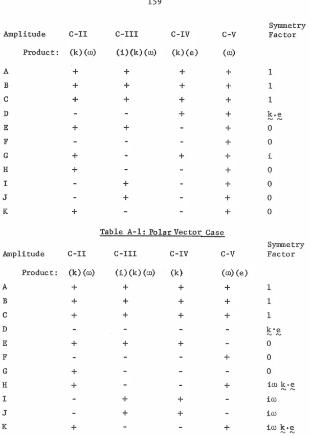
Polar vector case [synnnetry factors for an 159 axisynnnetric power spectrum].

I. INTRODUCTION AND SUMMARY OF RESULTS

A. Introduction

Cosmic rays are energetic particles of extraterrestrial origin. Their existence was first reported by Hess in 1912 and confirmed during the 1920's by an ingenious series of experiments by Millikan, who gave the name "cosmic rays" to the observed extraterrestrial radiation. (For a history of cosmic-ray research through 1964, see Rossi, 1964.) It has only been in the last few decades, since the advent of satellite and balloon observations, however, that intensive investigation o[ the properties of the primary cosmic rays has been possible. Since cosmic rays are the only samples of extraterrestrial matter that we have, apart from meteorites and moon rocks, they have proven extremely valuable in inferring properties of astrophysical objects.

For the purposes of this Thesis, I will limit the discussion to charged particles. The charged particles observed near earth are predominantly protons ("'95%), although heavier nuclei and electrons are also present. Local observations indicate that the primary cosmic rays are isotropic, and studies of electron synchrotron emission using radio telescopes show that the cosmic-ray flux is reasonably constant through-out the galaxy. Studies using measurements of induced radioactivity in meteorites conclude that the local flux is fairly constant over time

scales of the order of a million years. The observed cosmic radiation is therefore constant over long periods of time in our galaxy.

much longer than the rectilinear transit time for unscattered particles.

Energy considerations and the lack of observed gamma radiation from

the scattering of hypothetical extragalactic cosmic rays off of the

cosmic 3°K blackbody continuum indicate that the source of the major

portion of the cosmic rays lies inside our galaxy. Although the details

of the mechanism for cosmic-ray acceleration are not understood, it is

widely believed that cosmic-ray production is in some way connected with

supernova explosions and the remnants which they leave behind. (For a

continuing review of these points, see Ginzberg and Syrovatskii, 1964,

Ginzberg, 1969, Ginzberg, 1970, and Syrovatskii, 1971.)

Since supernova events are rare (~l per 50 years in our galaxy)

and the typical cosmic ray spends many rectilinear transit times in the

galaxy, there must be considerable scattering of the cosmic rays in

their propagation from the sources to the point of observation near

earth. The mechanism for this scattering process most likely involves

"collisions" with irregularities in astrophysical electromagnetic fields,

since ion-ion and ion-neutral collisions are rare and the gravitational

force on individual particles is negligible. Since scales of interest

in astrophysical discussions of cosmic rays are much larger than the

Debye length, and since the velocity of cosmic rays is much larger than

~

the Alfven speed or the speed of magnetohydrodynamic waves, the major

influence on the propagation of cosmic rays in interplanetary and

inter-stellar space is the magnetic field. Therefore, the scattering of

high-energy particles by irregular magnetic fields is an ir1teresting

magnetic fields and cosmic rays in interstellar space, much data exist for particles and fields in interplanetary space near earth. For this reason, I will subsequently·consider the scattering of cosmic rays by magnetic fields in interplanetary space, although the same kind of mechanism presumably applies also in the interstellar medium. A

schematic picture of interplanetary space in the vicinity of the solar equatorial plane is indicated in Fig. I-1, taken from Jokipii (1971). The "solar wind" is an outflow of plasma from the sun. It is composed

-3

primarily of protons (~5 cm near earth) and electrons flowing radially away from the sun with velocity V ~ 350 km/sec. The interplanetary

w

magnetic field is, on the average, an Archimedes spiral (Parker, 1963), with large fluctuations. Cosmic rays incident from interstellar space are scattered by the magnetic irregularities and become nearly isotropic in the rest frame of the outflowing plasma. The sun is occasionally an important source of particles with kinetic energy T ~ 10 MeV/nucleon, during solar flare events, and it may be a continuous source of particles with energies T ~ 10 MeV/nucleon~ A quantitative theory has been

developed to relate the average cosmic-ray distribution function to properties of the interplanetary medium, and the resulting diffusion equation has been useful in analyzing such phenomena as the 11-year variation in the cosmic-ray intensity, cosmic-ray anisotropies and gradients, and the time history of the cosmic-ray flux during impulsive solar flare events. (See the thorough review of these topics in

Figure 1-1: Schematic view of the interplanetary magnetic field projected into the solar equatorial plane. Rotation of the sun at angular speed

Oe

-1

... ...

Figure I-1

'

well understood in terms of this model. On the shorter time scale, on

the order of hours or days, however, the cosmic-ray flux is also

observed to vary, even during "quiet" times in interplanetary space.

It is the purpose of this Thesis to inquire about the

characteristics and the origin of broad-band cosmic-ray fluctuations

and to see if these short-term fluctuations can be analyzed in a manner

which can provide useful infonnation about the cosmic rays and the

plasmas through which they propagate. This type of investigation has

not previously been pursued systematically. Generally, the "noise" in

the cosmic-ray counting rate has been ignored or explored in an ad hoc

manner. Here I review the use of power spectra as a systematic scheme

for analyzing the data and then present the first quantitative models

of physical processes by which the broad-band cosmic-ray fluctuations

may be produced. This Thesis has basically two major parts. The first

is an analysis of several different types of cosmic-ray data to show

that the fluctuations are an interesting and persistent feature of the

cosmic-ray flux for a wide range of energies and frequencies. The

second part is the construction of quantitative models for the production

of cosmic-ray "scintillations" by interplanetary and magnetospheric

magnetic-field fluctuations and the demonstration that the observed

scintillations are in good agreement with the results of the

By scintillations, I mean the fluctuations in intensity which a cosmic-ray detector sees as a function of time while pointed in a given direction in space. The use of the term "scintillations" to describe this type of fluctuation will be clarified in Chapter III, where the similarity between cosmic-ray "scintillations" and

inter-planetary scintillations of radio waves will be discussed. The physical picture is that cosmic rays are guided along magnetic field lines. The cosmic-ray intensity varies as a functioa of time, because as the direction of the field varies different particle intensities are brought into the detector~ viewing cone .if there is a field-aligned anisotropy. Thus the magnetic-field fluctuations snd a cosmic-ray anisotropy cause cosmic-ray scintillations.

The quantitative description of this phenomenon begins with Liouville's equation for the conservation of particle density in

phase space,

d£

[a_

+

.L

+

-~J

<~-'

=

o .

(1)

Here the coordinates are position, (~),momentum (£), and time (t); ~ is the particle velocity, f(~,£,t) is the distribution function of particles in phase space, and d£ is the force. As discussed above,

dt

interest in interplanetary space in Chapters III - V below.

Chapter II is a discussion of the observation of cosmic-ray

scintillations. It begins with a discussion of the theory of stationary

random functions and the calculation of power spectra. Using this

framework, I then present power spectra of cosmic-ray counting rates

from several types of detectors. Power spectra are presented for

low-energy (1-40 MeV) protons inside the earth's magnetosphere, low-low-energy

(1-10 MeV) protons in interplanetary space during a solar flare, the

Alert and Deep River Neutron Monitors, interplanetary >50 MeV protons

together with

>4

All these types of data exhibit scintillations that are significantly

above the noise level, and it is found that relative scintillations

(i.e., fluctuations divided by average flux) are dependent on particle

species and energy but are generally independent of time for a given

species and energy during undisturbed periods in interplanetary space.

For.protons, scintillations are a rapidly decreasing function of energy,

and the contribution to the scintillations from processes near the

earth (inside the earth's bow shock) seems to be important for low

energies (~1-10 MeV).

The theory of magnetic-field-induced cosmic-ray scintillations

is discussed in Chapters III - V and the Appendices. Chapters III and

IV give the simplified theories of magnetospheric and interplanetary

scintillations, respectively, while the more general theory of

inter-planetary scintillations is presented in Chapter V and the Appendices.

Chapter III is a discussion of the theory of

perturbed regions of interplanetary space and the magnetosphere. The model is appropriate for cosmic rays with cyclotron radius and

mean-free-path large compared to the thickness of the slab, or for protons with T ~ 1 MeV. The model leads to an equation for the cosmic-ray

fluctuations in terms of average cosmic-ray gradients and the magnetic-field fluctuations, and its result is so similar to the equations for the interplanetary scintillations of radio waves that the term

scintillations is borrowed to describe cosmic-ray fluctuations. It is shown that the observed scintillations of the 1-40 MeV flux inside the magnetosphere can be reasonably understood in terms of the thin-slab model of the magnetosheath. The magnetosheath fluctuations cannot be

the source of the observed neutron-monitor scintillations becau:>e they decrease too rapidly with energy.

Chapter IV gives the theory of the interplanetary scintilla-tions of cosmic rays in the low-frequency limit: m, ~ ·~ << m

0. The model assumes that cosmic rays spend many scattering times in tile

detectors with equatorial asymptotic viewing cones, however, there is a

predicted enhancement in the power spectrum near a frequency of l/day

and a cutoff for lower frequencies. Taking these effects into account,

I show that all the major features of the power spectra of the Alert

and Deep River Neutron Monitor fluxes are explained by the interplanetary

scintillations model, including a prominent feature for Deep River near

f = 1/day. The model of interplanetary scintillations is in excellent

-7 < ~ -4

agreement with the observations for frequencies 5 x 10 Hz ~ f ·~ 10 Hz.

A mathematically more detailed consideration of the theory of

interplanetary cosmic-ray scintillations is given in Chapter V, where

the simplifying assumptions of Chapter IV are generalized and the

scintillation equations are considered in their general form for

arbitrary ~ and m. It is shown that the usual quasi-linear approach is

inadequate due to the strong resonant interaction between cosmic rays

and the magnetic-field fluctuations near the cyclotron-resonant

wave-number. A generalization of the quasi-linear equations, incorporating

the effects of the non-linear interactions explicitly, is developed.

The choice of an appropriate coordinate system reduces the problem to a

simple differential equation in one variable, and the solution is

obtained. It is shown that the interplanetary scintillations seen by an

omni<lirectional detector will be quite different from those seen by a

unidirectional detector. For conditions typical for 1 GeV protons near

earth, in the limit k

=

the average magnetic field), the more detailed consideration of the

resonant interactions in Chapter V differs only slightly from

and the solution to the problem involves the use of techniques of

non-linear plasma theory, the simpler theoretical framework of Chapter IV

adequately describes the physical processes involved.

Further details of topics related to those covered in the

text of the Thesis are given in three Appendices. Appendix A contains

a derivation of the most general allowed form of the magnetic-field

power spectrum, using symmetry properties and assuming that the

fluctuations are axially symmetric. Appendix B gives a new derivation

of the diffusion equation for the average cosmic-ray distribution function

using the techniques of Chapter V. The general form of the diffusion

coefficients is derived, allowing arbitrary axially-synrrnetric

magnetic-field fluctuations, and the result agrees with those of Hall (1967) and

Hasselmann and Wibberenz (1968). In Appendix

c,

for including the non-linear terms in the scintillation equations of

Chapter V is discussed. Following Rudakov and Tsytovich (1971), I

introduce an effective scattering operator into the equations and then

iterate to obtain an expression for the lowest-order non-vanishing

contribution of the non-linear terms. The result is a resonance width

which depends on frequency but which is of the same approximate size as

the widths obtained by dimensional analysis in Chapter V. The conclusion

that the low-frequency limit of Chapter IV applies for frequencies up

-4

to 10 Hz for 1 GeV protons in interplanetary space is strengthened by

c.

The purpose of this Thesis is to investigate, for the first

time, cosmic-ray scintillations in an attempt to discover their origin

and to consider their possible uses as probes of astrophysical

electro-magnetic fields. The theory of cosmic-ray scintillations in the

magnetosphere and in interplanetary space was developed, and it was

shown that the theory is in good agreement with power spectra calculated

from several types of cosmic-ray data. The validity of the models used

seems to have been reasonably established, so that it is safe to conclude

that the origin of cosmic-ray scintillations under most circumstances is

in random interplanetary magnetic fields and their scattering and

focusing of cosmic-ray trajectories.

If this interpretation is valid, several important points can

be made concerning the utility of cosmic-ray scintillations as a probe

of astrophysical plasmas. First, as shown in Chapter III, low-energy

(~1-10 MeV) proton scintillations inside the magnetosphere are related to the cosmic-ray anisotropy and to the magnetosheath magnetic-field

fluctuations. Since most space probes spend little time passing through

the magnetosheath, low-energy cosmic-ray scintillations may be a useful

tool in obtaining information about the magnetic-field configuration and

its variation in the magnetosheath.

Similarly, as shown in Chapters IV and V, scintillations for

cosmic rays of neutron-monitor energies (~l GeV) are related to the cosmic-ray anisotropy and interplanetary magnetic-field fluctuations.

obtain information about the interplanetary magnetic field when direct

observation is not possible. In particular, neutron-monitor data are

available for time periods during the 1950's and the 1960's when little

interplanetary magnetic field data are available. High-counting-rate

neutron monitors can be used to extend the investigation of

scintilla--4

tions to frequencies larger than 10 Hz, and in many cases the <lata are

already suitable for analysis and thus provide an inexpensive source

of possibly interesting information.

An immediate consequence of the excellent agreement between

the theory and observation of interplanetary scintillations is the

validation of the basic theoretical· structure underlying the model.

Thus, the standard picture of cosmic-ray propagation and diffusion in

interplanetary space (Jokipii, 1971) has passed a rather stringent test.

As indicated in Appendix B, the Fokker-Planck diffusion equation is

based on the same set of assumptions as the scintillation equatjons.

Whereas some other observational tests of the diffusion theory - such as

radial gradient measurements, for example - are difficult to perform,

the "scintillations test" described here simply involves comparing

cosmic-ray and interplanetary magnetic-field power spectra.

Finally, as shown in Chapter V and Appendix

c,

scintillations may be an ideal testing-ground for non-linear plasma

theories. In the cyclotron-resonant regime, the contribution of the

non-linear terms is quite large. Although neutron monitors hav<'. too

large an energy response (and hence too broad a cyclotron resonance)

-4

agreement between theory and observation for frequencies up to ,,10 Hz

indicates that the method of including the non-resonant terms in the

resonance width as presented in Chapter V and Appendix C is approximately

correct. It is possible that other detectors could provide a meaningful

test of non-linear plasma theory, since the average distribution function

is well understood and the non-linear effects are very important near

the cyclotron resonance.

Thus, there are many valuable avenues of research to which

II. OBSERVATIONS OF COSMIC-RAY SCINTILLATIONS

An inspection of the cosmic-ray flux measured by a given

detector as a function of time reveals fluctuations even during "quiet"

times in interplanetary space. In this chapter, I introduce the subject

of power spectral analysis as a means of quantitatively describing the

nature of the fluctuations. I then present analyses of several different

types of cosmic-ray data and show that in each case the scintillations

are larger than can be explained on the basis of Poisson fluctuations

alone.

A. The Theory of Stationary Random Functions

In order to develop a statistical framework to evaluate random

fluctuations, imagine an ensemble of independent systems which are

identical in all respects except that the random fluctuations in each

member may be different. Each member of the ensemble is called a

realization, and a typical realization may be as shown in Fig. II-1. The

random function at each instant of time t can be averaged over the

n

entire ensemble of realizations to yield the average value x

0(tn)' and

the fluctuating part of x is given by

(la)

with

(lb)

and (a) represents the ensemble average of any random function a. A

random function is one which can be visualized as being composed of many

Figure II-1: Stationary random function. An illustration of a

station-ary random function, x(t). The mean is x and the fluctuating

0

part of x(t) is x

1• The correlation time T c is the time after

which the function at t + T is no longer correlated with the c

0

x-~

as stationary if all of the moments (x(t)j), j=l,2,3 .... are independent of time. In practice, weakly stationary (or que$i-stationary)

random functions - random functions whose ensemble average varies, but on a time scale much longer than the correlation time of the fluctuations -are often encountered and have the same basic properties as perfectly stationary random functions.

In most cases of physical importance only one realization is obtained over a period of time. In order to utilize this data, it is necessary to append the ergodic hypothesis to the definition of the random functions. The ergodic hypothesis simply states than an ensemble average is equivalent to a temporal average over any one realization if the temporal average is taken over a long enough period of time. That is, for arbitrary a(t), the ergodic hypothesis is equivalent to the equation

T

(a(t)) _lim

;TI

T-t(X) -T

a(t

+

( 2)

Under the ergodic hypothesis, x

0 for a stationary random function is simply the temporal average of the function.

The autocorrelation function, or simply the correlation function, is defined as

(3)

Since x

tion function is flat near ,.. = 0. The time T beyond which the

correla-c

tion function falls off rapidly is called the correlation time, and it is shown schematically in Fig. II-1. ·

The Fourier transform of the correlation function is called x

the power spectrum, P (ro):

-cc

and the inverse transform gives

I

2rc e ro .

-(X)

(4)

(5)

The power spectrum is an even, positive-definite function of frequency, ro. From the theory of Fourier transforms, .it follows that the "spread" in frequency space over which the power spectrum is near its maximum value is given by

ro rv l/ 'T ¥

c c

For a rigorous discussion of the topics in this sections, see Yaglom

(1962). The power spectrum is a quantitative measure of the frequency distribution of the fluctuations being consideredo

equation (2) is replaced by an expression in which the right side involves integrals over x', y', and z' as well as t'. In equation (3), the

correlation function becomes a function of the four separations

s

~

and the right-hand side becomes (x₁ (~,t) x₁(£

+

+

T)).

Most cosmic-ray data are composed of a set of discrete,

equally-spaced, counting rates. For simplicity, only this type of data will be

discussed here. Since information is available only once every T time

units, it is evident that such data can contain no information for

frequencies larger than l/T. Actually, since Px(m) is an even function

of frequency, half of the information content in the data is redundant

and consequently only information about frequencies

*

f ~ f - l/2T (6)

•k

is available. The frequency f is called the aliasing frequency. Let

T be the total length of the data record, so that there are n I/T

equally-spaced data points in the record to be analyzed.

As is conventional, the observed power spectrum will be

considered a function of frequency in the range 0 ~ f <

oo,

x

with equation (4) and the even nature of P (f) yield

4

I

0

(7)

Since the correlation function at zero lag, Rx(T

=

variance a2, it is easy to show from equation (5) that the variance

of x(t) and the power spectrum are related via

2

(8) a

Although the measured power spectrum contains no information

*

about frequencies f

>

frequency. In essence, the collection of data at times separated by T results in the folding of the entire frequency range 0 ~ f < oo onto the

*

smaller range 0 ~ f ~ f in an accordian-like manner. The calculated power spectrum pX(f)

1 1 d will be related to the true power spectrum ca cu ate

Px(f) by

Px(f)

calculated

c:e

Px(f) + 2: j=2 even

x

*

P (jf -f)+P (jf +f) (9)

This "aliasing" of the spectrum is a result of gathering data at discrete points and is independent of the method used to estimate the power

spectrum. For a power spectrum falling off as f-p for f

~

1 -1~

over the entire frequency range and less than 10% for f <

2-f .

fall off rapidly enough that aliasing is unimportant.

Given an equally-spaced (in time) series of data points, there are three commonly-used methods of calculating power spectral estimates. The first is the "fast Fourier transform" method. Given a function x(t) from time t

=

=

1,,

x ~ ~

*

2~P (ill) o(ill - ill') = (x(ill) x(ill') ), (10)

independent estimates, each with better statistical accuracy.

The second method used to calculate power spectra is the

"correlation-function" method, discussed in detail by Blackman and

Tukey (1958). For an asympotitically large number of data points, the

Blackman-Tukey algorithm produces the same results as the fast Fourier

transform method and has the same statistical properties. The method

is based on equations (3) and (4); first the correlation function

R~(T) is calculated form values of T, and then R~(T) is

Fourier-i i

transformed as in equation (4) to obtain m estimates of the power

spectrum. The estimates are then smoothed to produce new estimates

with slightly better statistical properties. (In the applications

discussed below, smoothing in the frequency domain is done using the

"hanning" algorithm.) It can be shown that the number of degrees of

freedom that each of the m power spectral estimates has is 2n/m, and

the errors in the estimates have a chi-squared distribution with 2n/m

degrees of freedom. In practice, estimates are usually made with at

least 10 degrees of freedom so that the errors are not too large. If

too few degrees of freedom are allowed in the calculation, the algorithm

can produce such spurious results as power spectra which are negative

over some range of frequencies.

A third method of calculating power spectra is the

nested-var-iance method, called the pilot method by Blackman and Tukey. Its first step

is to calculate the variance (cr 1

2

) obtained from consecutive intervals

of duration T. Next one calculates the variance (cr 2

2

) obtained from

t+T 2

«.!.

I

«'

t

and

t+2T 2

((~T

I

(O' 2 ) = (llb)

t

Then it can be shown (Siscoe and Jokipii, 1966) that

0)

I

r

J

- 2rt rtfT

0

(12)

The function in brackets is a rather sharply-peaked function of

•k

*

frequency with maximum located at f ~ 0.7f, where f

=

*

~ (4rt/f )

c<cr1 ) -

Thus the'calculation of two variances gives an estimate of the power

*

*

spectrum for frequencies between f /2 and f . If one next calculates the variance (cr

4 2

) from consecutive intervals of duration 4T, one can use equation (12) with the substitutions ( 012)-( 022),( 022)-( 042), and T - 2T. An estimate of the power spectrum for frequencies between

'"J'c

*

f /4 and f /2 is then obtained. The procedure can be continued to give p-1 estimates of the power spectrum at p-1 frequency intervals going

•/(

spectra by the nested-variance technique is straightforward. For

Gaussian statistics, or for any statistics if the number of data points

n is large, it can be shown that the variance (cr 1

2

) is distributed

according to the chi-squared distribution with n degrees of freedom.

Similarly, ( 022) has a chi-squared distribution with n/2 degrees of

freedom since only half as many data points are available. Since the

difference Xs2 - xt2 between two chi-squared distributions withs and t

degrees of freedom respectively is again chi-squared with the number of

degrees of freedom given by (s-t) (e.g., Section 2.6 of Theil,

1971), it follows immediately from equation (13) that the P?Wer-spectral

estimate indicated has a chi-squared distribution with n/2 degrees of

freedom. The next estimate, based on (a 2

2

) - (cr 4

2

), has a distribution

of

Xn

4

with n/2j degrees of freedom.

It is instructive to compare the types of estimates of the

power spectrum obtained by the correlation-function and the

nested-variance methods. For a data record with n points, the

correlation-function method with 20 degrees of freedom yields approximately m = n/10

*

estimates of the power spectrum, equally spaced by intervals of lOf /n

in frequency space. The nested-variance method yields p estimates of

the power spectrum, where n = 2P, and the estimates are equally spaced

in log f since they correspond to frequencies differing by factors of

two. Therefore, if the power spectrum is to be plotted on a log-log

method of finding estimates is more appropriate. In both cases the

observed power spectrum is obtained from a convolution of the true

power spectrum with a "filtering" factor in frequency space. The

correlation-function method's banning filter is described in Blackman

and Tukey (1958), and the nested-variance filter is the term in brackets

in equation (12),

~

i<j

2

sin 2.f/f

Q(f)o:-

*

'

(~f/f )

(14)

*

where f . is the aliasing frequency, l/2T. A comparison of the frequency

filters of the two methods is shown in Fig. II-2, where two decades of

frequency are shown and it is assumed that m

=

the correlation-function method. Notice that, on the logarithmic scale

used, the nested-variance method's filter has the same shape for all

frequency bins, whereas the correlation-method's filter shape gets

narrower for larger frequencies. In both cases, however, the filter has

decreased to about 80% of its maximtnn value at the ends of the nominal

width of the frequency band and has a value of less than 20% of its

maximum in the second frequency band away from the central one. Both

-2

filters fall off approximately as f far from the central frequency,

indicating that these methods are inaccurate if the power spectrum falls

-2

Figure 11-2. Frequency filters for power spectral analysis. A com-parison of the frequency filters for the correlation-function method (solid curve) and the nested-variance method (dashed curve) of calculating power spectra~ Ten estimates are used in the cor-relation-function method, and a logarithmic frequency scale is usede The vertical scale is lineare The two divided lines at the top of the figure give the nominal widths of the frequency

mC--r~~~~~~~~~-O

ro

l'-lO

LO

~

C\J

0

/

C\J

\

/

_,,_,.

----==-~-==---::...:---:

---

---

---'

'--.---~

.

z

t0

0

w

·

~

0

<(

z

_J <(

~ ~

a:

0::

<(

0

>

0

'

'

'

'

'

'

'

'

~3111.:J

---

---LO

C\J

*

'

-"

'+-0

LO

.

0

C\J

Consider a detector which samples an average· counting rate of

n particles/sec for t sec. For Poisson statistics, the expected

relative mean-square error of the total number of particles counted will

be

N 1

=

=

N2 N 1

nt (15)

An important property of Poisson statistics is that each observation is

completely independent of the previous time-history of the system, so

the frequency spectrum must be flat. As discussed above, the power

*

*

spectrum is defined for frequencies 0 ~ f ~ f where f l/2T. Another

property of the power spectrum, as shown in equation (8) above, is that

·the variance is the integral of the power spectrum over all frequencies.

From these properties of Poisson statistics and of power spectra, it is

straightforward to show that the power spectrum of the relative

flue-tuations oN/N is given by (Owens and Jokipii, 1972)

P(f)

=

p 0 ~ f

s

*

Here D

=

cycle during which data are collected by the detector.

For a detector, such as any cosmic-ray detector, which samples

particles subject to Poission counting statistics, the Poission power

indicated by equation (16) is the minimum or noise level. Any other

mechanism which causes fluctuations will cause frequency-dependent

increases in the power spectrum over the level indicated by equation (16).

will be discussed below. Power spectra which exceed Poisson power over some range of frequencies therefore exhibit statistically significant fluctuations. In order to facilitate comparison both with the Poisson noise level and with the results of the theory presented in the later sections, I present power spectra of the relative fluctuations (i.e., x

1/x0 in the notation of Section II.A above) of the cosmic-ray counting rate. Data for which power spectra may be calculated must satisfy several general requirements. The process must be approximately

stationary; that is, the average value of the cosmic-ray counting rate must be constant or vary slowly over the time scale to be investigated. Data must be available at fixed intervals, with few data gaps. Finally, for the spectra to be physically interesting, the counting rate must be high enough so that fluctuations merely due to Poisson counting

Counting rates of low-energy protons from polar passes of a low-altitude polar orbiting satellite (OGO VI) were graciously provided by the Caltech group under the direction of E. C. Stone and R. Vogt. A solid-state detector with an effective threshold of about 1 MeV/nucleon and an upper cutoff of about 40 MeV for protons (150 MeV/nucleon for alpha particles) was used to sample the counting rate at terrestrial latitude greater than 74 degrees on each polar pass. The rigidity cut-off for 1 MeV protons in the magnetosphere during quiet times occurs at less than 72 degrees latitude, so temporal variations are due to a

variation in the flux of cosmic rays and not to varying geomagnetic cut-offs. The data-collecting time was about eight minutes over each pole, and the transit time between poles was about 50 minutes. The fraction of the counting rate due to alpha particles was less than 5% and there was essentially no electron contribution, so that essentially the entire

flux measured is due to protons with kinetic energies 1 MeV ~ T ~ 40 MeV. The counting rate during quiet times was typically one count per second, or 500 protons per polar pass. The orbital parameters were such that a certain fraction of the orbits were too far from the poles for polar data to be gathered and analyzed. Therefore, it was necessary to average over several polar passes to obtain data points which were equally spaced in time.

fitted to the data and subtracted to remove the average and the linear time trend, and power spectral analyses were performed separately for three representative quiet times. The relevant parameters for the three

periods selected are presented in Table II-1.

The power spectra for the three periods given in Table!I-1 are given in Figures II-3, II-4 and II-5 as indicated. In Fig. II-3, I have presented power spectra calculated on the identical data from both the correlation-function method (circles) and the nested-variance method

(histograms).. It can be seen that the two methods of calculfl,ting the spectrtnn are in basic agreement, with a frequency spectrum going

-2

approximately as f • The spectra in Figures II-4 and II-5 have about the same shape as the one in Figo II-3 and amplitudes which are nearly the same, in spite of a factor of 10 variation in the average flux as shown in Table II-1. The power spectra for all three periods are superimposed in. Fig .. II-60 It is clear that the three spectra coincide quite well, indicating that the relative quiet-time low-energy cosmic-ray fluctuations are a persistent feature, changing little in amplitude

-6 <

<

(for frequencies

10

1

about

2

V

1

2

)

inside the magnetosphere at these energies is proportional to the average flux j

0• That is, the observations establish the criterion that (17)

(counts/sec) (Hz-l)

Cl Sept. 19-25, 1969 So 3.

C2 Nov. 11-21, 1969 0.4 30

C3 June 22-July 15, 1969 lo 15

Table II-1

II-3

II-4

II-5

I

o

5

,.---Cf

---:>

z

-0:::: I

o

3

w

s

0

()_

I

o

2 _ _ _

____.._____ _ _

---'

10-6

10-5

10-4

0

J

"

-J

Z

.

C2

-

10

3

0:::

w

3

0

Q_

102 ...__ ____

....,___ _ _

,___,,

10-6

10-5

10-4

Figure II-5. Power spectrum of the 1-40 MeV proton flux, C3. Data

taken during a quiet time aboard OGO VI, June 22 - July 15, 1969,

The average counting rate was l/sec and the Poisson noise level

-1

105

r r

-~

-I

N

4

I

10'

~

0

J

'

J

-z

103

-Ck

w

C3

I

3

0

o_

I

o

2 ....__ _ _ _

_ _ J

10-6

10-5

.

10-4

Figure II-6. Power spectra of the 1-40 MeV proton flux, Cl, C2, and C3. Power spectra from the last three figures are superimposed on one graph, with coding indicated on the figure. The straight line is a visual best-fit to the data. Below 10 -5 Hz, the dashed extension

-2

~

-I

N

¢

0

J

"

105

10

4

_, 10

3

.

z

0:::

w

3

0102

Q_

\

-t-CI

I

--t--

C2

'

'

r----1

C3

10

L---L---~---~----10-6

10-5

10-4

10-3

must satisfy.

The power spectra presented in Fig. II-6indicate that the fluctuations are much larger than expected on the basis of Poisson counting statistics alone. The Poisson noise level for each spectrum, as calculated from expression (16), is indicated in Table II-1, and the observed power spectra are all a factor of 10 or more larger. The shape of the power spectrum of ~1-40 MeV proton scintillations inside the magnetosphere is approximately a power law in frequency with exponent of

(-2) for f

~

(18)

where Pj(f)/j 0

2

is the power spectrum of j

1/j0 in the notation of Section II.A above.

Williams (1969) has obtained power spectra of 1-10 MeV protons in interplanetary space during solar flare events. A typical spectrum, for Nov. 15-16, 1967, is shown in Fig. II-7. Although this spectrum was taken during a non-quiet time in the interplanetary medium, so that the fluctuations might be expected to be larger than normal, a comparison with Fig. II-6 (for 1-40 MeV protons inside the magnetosphere) shows that

the interplanetary spectrum (even though obtained during a disturbed period) is about an order of magnitude lower in amplitude than the spectrum observed near earth. This may be an indication that the major source of low-energy cosmic-ray scintillations near earth is the

Figure II-7. Power spectrum of the 1-10 MeV proton flux. Data taken during a solar flare in interplanetary space by a detector aboard Explorer 34, on Nov. 15-16, 1967. Power spectrum given by Williams and renormalized to give the power in j

1/j0 • The average counting

I

N

:I::

..

·-'

·-

c

·-102 __________________________

~---10

I I I

I

I

,,

/

I

EXPLORER

95%

f

Interval

---i

10

Poisson noise. Although further data, particulary simultaneous

measurements at similar energies inside and outside the magnetosheath,

are necessary before any definite conclusion can be drawn, it appears

that the scintillations of cosmic rays of low energies (~l-40 MeV) may

be much larger inside the magnetosphere than in interplanetary space

E. Scintillations of High-Energy Protons (T~ 1 GeV) and Electrons (T ,... 5 MeV)

Neutron monitors are cosmic-ray detectors on earth which count neutrons produced as secondaries in the interaction of high-energy cosmic rays with the earth's atmosphere. Neutron monitors respond primarily to cosmic-ray protons with energies T

0 ~ T ~ 50 GeV incident at the top of the atmosphere, where the threshold value T₀ is called the geomagnetic cutoff energy and depends on the location of the neutron monitor in the earth's approximately dipole magnetic field. The calculation of the geo-magnetic cutoff and of the detailed energy response of the monitors

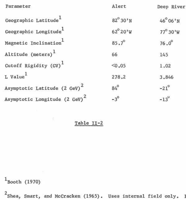
de-pends on the geomagnetic field and the cosmic-ray energy spectrum, and such calculations have been done previously (see, for example, Shea, Smart and McCracken, 1965). The relevant data for the two neutron

monitors used in this study are given in Table II-2. It can be seen that the Alert Neutron Monitor responds primarily to particles with the same asymptotic direction in interplanetary space (corresponding to geographic latitude ~

60°),

In order to facilitate comparison with the low-energy data, I have analyzed the counting rates of the Alert and Deep River Neutron Monitors for the period Sept. 1-Nov. 30, 1969, a period which includes

Parameter

Geographic Latitude1

Geographic Longitude1

M agnetic Inc ination • i· . 1

1

Altitude (meters)

Cutoff Rigidity (GV)l

L Value1

Asymptotic Latitude (2 GeV)2

Asymptotic Longitude (2 GeV)2

Table II-2

Alert

82° 30'N

62° 20'W

85 07°

66

<0.05

84°

Deep River

46° 06 'N

77° 30'W

76 00°

145

L02

30846

-21°

1

Booth (1970)

2

Shea, Smart, and McCracken (1965). Uses internal field only. For

extended geomagnetic tail, variation in asymptotic latitude

Monitor is given in Fig. II-8. Of the two spectra in this figure, one

was calculated after subtraction of a fitted straight line and the other

after subtraction of only the average. The close correspondence between

the two spectra indicates, as expected, a lack of dependence of the

power spectrum on the method of removing long-term trends in the data.

The shape and amplitude of the power spectrum are approximately given

by

(19)

The power spectrum of the Deep River Neutron Monitor is given

-6

in Fig.II-9 for frequencies f

>

using both the nested-variance method (histogram) and the

correlation-function method (open circles)~ The overall shapes of the two spectra

in this figure are the same, but there are differences in detail. Near

f

~

cor-relation-function method indicates a peak; this peak will be discussed in

Chapter IV. The well-known diurnal anisotropy appears as a small, sharp

spike in the power spectrum (Ables, 1967) which is unresolved in this

anal-ysis. Thus, the diurnal anisotropy is only a small perturbation to the

power spectrum and not the dominant effect. Thus, it can be concluded that

statistically-significant scintillations are exhibited by neutron monitors,

indicating fluctuations in the cosmic-ray proton flux at ~2 GeV kinetic

energyo Power spectra of neutron-monitor counting rates over more

restricted frequency ranges have previously been presented by Dhanju

and Sarabhai

(1967)

Figure II-8. Power spectrum of the flux of the Alert Neutron Monitor.

The solid points are obtained from the raw data after subtraction of a fitted straight line. The points marked X are the power spectrum obtained from the same raw data after subtraction of the mean only. The period is Sept. 1 - Nov. 30, 1969, and the average

·counting rate was about 180/sec. The noise leve 1 was rv 10 -2 Hz -1 e

-

N

:::c

...

0

"-

·--z

0::

w

~

0

a_

10

ALERT

10

t

10-2...__ _ _ _ __._ _ _ _ _ _..._ _ _ _ _ ...__ _ _ _ ____

10-

10-

10-

10-

10-

Figure II-9. Power spectrum of the flux of the Deep River Neutron Monitor. The solid histogram is the power spectrum obtained with

the nested-variance method. The open circles are the power spec-trum obtained with the correlation-function. The period is Sept. 1 - Nov. 30, 1969, and the average counting rate was about 510/sec .

0

10

I

N

6

0

~I

z

0:::

w

$10-I

0

o_

DEEP RIVER

I

90%

0

0

0

0

o~

'9

Monitor flux for frequencies 1/11 years ~ f ~· l/hour. His spectrum

agrees with those presented here, and the discussion in Chapter IV below

will consider his high-resolution spectrum near f ~ l/day in detail.

The power spectra of the Alert and Deep River Neutron Monitors

are superimposed in Fig. II-10. It can be seen that the shapes and

ampli-tudes are basically the same, with a few differences in detail. Near

-5

10 Hz, the excess of the Deep River over the Alert power can be

ex-plained on the basis of the much larger diurnal anisotropy seen by the

former and by effects of the earth's rotation (see SectionIV-B). The

coincidence of the spectra indicates a non-local origin of the

scintil-<.. -2 -1

lations, and the noise level of ""i x 10 Hz indicates that the

scin-tillations are statistically very significant. The scinscin-tillations can

be reasonably well approximated by equation (19) for frequencies

-7 .. -4

5 x 10 Hz~ f ~ 10 Hz. A comparison of equations (19) and (18)

indicates that the scintillations are much larger for ""l MeV protons

than they are for ""l GeV protons; by a factor of over 1000. Although

the variation in jO was not large enough to establish that the relative

fluctuations are constant (i.e., that equation (17) is satisfied) at

relativistic energies as was established for low-energy protons; the

high-energy data are consistent with J<jl2

>

jo.

An attempt was made to determine the scintillations of

high-energy protons in interplanetary space from data provided by F. B.

McDonald and V.

K..

Figure II-10. Power spectra of the fluxes of the Alert and Deep River

Neutron Monitors. Power spectra from the last two spectra are

s~perimposed on one graph, with coding indicated on the figure.

9(fjo

·

indicated; those for Deep River are the same. The period is Septo 1

-~ov.-

-3 -1

7

N

:r

... -~

·

.

"

·--

c

....

I

0

c..

10

-2

10

10 ..

-+-Alert

-

Deep River

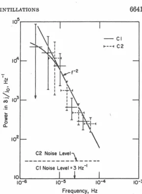
The instrumentation has been previously described (Balasubrahmanyan

et alo, 1965). The detectors essentially sample the omnidirectional

flux of cosmic-ray protons with energies above "'-'50 MeV and electrons

with energies above ,.._,4 MeV. The sampling time was approximately 5

minutes, and the average counting rate was 12 counts per second. The

power spectrum of the counting rate for a typical 20-day quiet period

in October, 1966 is given by the histogram in Figo II-11. (Ignore the

hexagons; these data will be discussed below.) The "noise" level marked

in the figure is that calculated from equation (16). It is evident

that Poisson noise dominates the spectrum (for this counting rate) for

f

~

Section II.C. There are significant non-Poisson fluctuations in the

-6

<

One might at first assert that the power spectrum of Fig. II-11

corresponds to high-energy protons, since the electron contribution to

the flux is about

s%

less than 5% for the detector used. However, simultaneous but

indepen-dent measurements of the electron flux (McDonald et al., 1972) indicate

that the electron componant varies by factors of order unity from day to

day, whereas the proton scintillations inferred from the neutron-monitor

measurements are in the order of 1% over the same period of time. To

evaluate the electron contribution to the power spectrum of the IMP 3 flux

shown tn Fig. II-11, I have calculated rough power spectra from the

pub-lished electron counting rates (McDonald et al., 1972) for the same period

of October, 1966. From daily averages of the electron counting rate, I